Sage Journals: Discover world-class research

Abstract

A framework is proposed in which certain well-known concepts of statistical mechanics and thermodynamics can be used and applied to characterize structural systems of interconnected Timoshenko beam elements. We first make the assimilation to a network of nodes linked by potential energy functions that are derived from the stiffness properties of the beams. Then we define a series of thermodynamic quantities inherent to a given structure (i.e., internal energy, heat, pressure, temperature, entropy, and kinetic energy). With the exception of entropy, all of them have the dimensions of energy. In order to test this new framework, a series of experiments was performed on four structural specimens within the elastic regime. Their configurations were taken from the seismic regulations known as Eurocode 8 in order to have a better based reference for our comparisons. The results are then explained within this new framework. Very interesting correlations have been found between the parameters given in the code and our concepts.

1. Introduction

1.1. Aim of the Research

The present paper explores the viability of employing concepts of statistical mechanics and thermodynamics as tools for the analysis of conventional structures.

Energy principles have been intensively employed in structural mechanics for several decades, either to obtain governing equations by means of variational methods or to justify different approximation methods (may references [1, 2] serve as examples). However, in practice, the goal of these methods is commonly limited to retrieve strains, stresses, and displacements. Such an approach omits the very important fact that, by treating problems of elastomechanics under the perspective of energy transfer and energy balance instead of only balance of forces, much valuable hindsight can be obtained regarding a structural system.

Very interesting and promising advances have already been made thanks to the observation of the behaviour in the energy domain in the areas of fluid-structure interaction [3], structural impact [4], or structural dynamics [5], to name a few.

In our case, the particular field of application will be earthquake engineering. Modelling seismic structural response as an energetic exchange process between the soil and the structural system has attracted the interest of many researchers in the past decades ([6 –8]).

In this work a series of structural configurations will be presented and compared based on quantities such as total work, internal energy, temperature, heat, kinetic energy, and entropy.

The conventional scope of such quantities is tied to the study of systems with a large number of nanoscopic or microscopic particles.

The information they provide about a system, however, can also be useful in the characterization of different macroscopic structural systems with a relatively small number of nodes. To such effect, however, some work needs to be done in order to adapt the existing tools for analysis.

We have resourced to a general purpose finite element application and modified it in order to retrieve the aforementioned quantities. We have defined a series of nodes where the distributed strains and stresses given by the constitutive model have been lumped. Our contribution allows treating models of beams as models of particles and applying the analytical techniques of statistical mechanics.

1.2. Another Field of Application of Statistical Mechanics

Statistical mechanics are widely used for the simulation and definition of material properties in many scientific disciplines.

In statistical mechanics, the elementary particles are molecules or atoms which are represented as point masses that are connected to one another by means of potential functions. These functions, together with velocities, allow for the computation of potential and kinetic energy states from which statistical data about the particles can be obtained and then used to characterize macroscopic behaviours.

Current research in the characterization of nanoscale structures ranges from the description of the properties of nanotubes of different elements (carbon, boron nitride, silicon,…) to that of polymer composites. References [9 –11] show how structural, elastic, and thermodynamic parameters can be defined for the study of the global behaviour of different materials from their atomic scale.

On the other side, in engineering practice, the most extended discretization methods are those which simulate matter by replacing it with pieces that interpolate the expected material behaviour (deformation, heat, etc.) between a series of nodes. Such are the techniques of finite elements, finite differences, or boundary elements, among many others.

These conventional continuum methods, however, are not applicable to nanoscale components because macroscale behaviour is incorporated in the constitutive models of solids, generally based on empirical results [12].

In their standard implementations, these methods provide the analyst information regarding the strain or stress states of links or “elements” between nodes (i.e., rods, beams, tetrahedra, etc.) but give no results regarding what happens in the actual nodes.

The main purpose of this paper is to provide means of translating those techniques employed in the representation of atomistic systems and make them available also for macroscopic systems.

1.3. The Thermodynamic Properties of Structural Systems

The branch of statistical mechanics which treats and extends classical thermodynamics is known as statistical thermodynamics. This discipline seeks to relate the microscopic properties of individual particles to the bulk properties of the sample which contains them.

In analogy, if a structural system is treated as a set of interconnected nodes, the global characteristics of its behaviour can be described by using probabilistic and statistical techniques.

By defining thermodynamic parameters for a structural system and establishing relationships between them, it is possible to expand our understanding of it in a more global manner.

Instead of just monitoring the internal tension distributions of particular beam elements or the displacements of a defined node, one can achieve a general view about how a whole system responds to a set of loads by computing, for example, its degree of “structural heat,” which summarizes in a single parameter both the internal stress distribution and the amount of displacement. These parameters are extremely valuable for the proper design of structures of any kind.

For the sake of simplicity, this study has been limited to Timoshenko beam configurations in two-dimensional frame-like structures. However, this scheme is a general one and can be applied to any kind of structure and to other types of discretization other than beam type finite elements.

Using statistical relations between the nodes, in the present paper the following thermodynamic variables have been computed:

the number of nodes, N,

the change of internal energy, dU,

the change of internal strain energy, δW,

the added heat, δQ,

the change in entropy, dS,

the temperature, T,

the quasistatic kinetic energy, KEqs.

The energy related quantities listed above are relatively straightforward to obtain, as will be shown in the following section.

For the definition of the entropy, due to the relatively small number of involved particles, N, we have had to resource to nonasymptotic thermodynamic ensembles. In this case, Boltzmann's equation for the definition of probabilities does not apply, so for the calculation of the probabilities of the nodal energetic states it was necessary to make use of a frequency based model adapted from references [13, 14].

1.4. Numerical Examples

The behaviour of four different structures with the same number of nodes but different topological complexity was investigated under a simple lateral load. Their description was based on widely used seismic regulations.

In the recent past, the research community of seismic structural analysis has made particular emphasis on the energetic aspects of the dynamic behaviour of the structures, so that currently the energy absorption capacity of a building is starting to be considered a good measure of its seismic performance.

For practical reasons, these behaviours are often synthesized in the form of coefficients that, conveniently applied, serve as tools for the analysts and designers. Many of these coefficients, however, are of empiric origin and their theoretical fundament is not always deeply explained.

As an example of the versatility of our methodology, we studied one of these parameters, provided by a broadly used design standard (Eurocode 8, [15]), as applied to our structural systems of choice. This parameter is known as the behaviour factor, q, and synthesizes the tendency of a given structural configuration to yield under the applied loads.

The space of possible states of each structure was explored by means of random iterations over the magnitude of the applied load. These variations allow for the observation of particular tendencies and correlations between the above-listed variables. The range of calculated values of these variables (KE,δW,δQ,dS,T) is shown as a function of the applied load, so that an outline of their response can be observed.

2. Elements of Statistical Mechanics for Structural Systems

In this section a set of quantities involving energetic terms will be presented for their subsequent application in the numerical examples.

In common structural engineering practice, the emphasis of the analysis is mainly done in stresses, strains, and displacements. This is due to the fact that the purpose of such analysis is to design, eventually, structural elements such as beams and columns. The global energetic behaviour of the structural system has been considered unimportant until recently and the acquisition of such data has not received the deserved attention.

What is presented here is a methodology to calculate elementary energy-related terms from a general-purpose finite element application whose relationship to the applied force can be later studied under the perspective of a thermodynamic exchange process.

The main hurdle is to associate the macroscopic constitutive models of beams to node-clustered points of energy. In particular, this is necessary to calculate the global values of internal work and entropy.

In general, the techniques employed in modelling microscopic structures explicitly set up molecular networks as atoms bonded by potentials. This facilitates the implementation of simulators of molecular mechanics. Some efforts have been done in associating those potentials with finite element method's elements ([12, 16]) and have successfully proven that the change of scale is possible.

The advantage of investigating energetic relationships between particles instead of particular changes in the bonds between them is mainly that of global perspective.

By treating structural systems with the techniques of statistical mechanics, we are making possible the identification of constants and patterns that would otherwise remain unappreciated.

Under the scope of thermodynamics, global continuous quantities and their behaviour are studied, providing a higher level of understanding when applied to macroscale systems such as built structures.

The first law of thermodynamics is an equation of change:

d U = δ Q - δ W,

(1)

where dU is the change in the internal energy of the system, δQ is the heat added to the system, and δW is the work performed on the system.

Within the proposed framework of this paper, the systems which are under study consist of sets of interconnected Timoshenko beams under the effect of static loads. By means of a general purpose finite element application, the linear equations which yield the displacement vector are solved, and the corresponding internal stresses and tensions are obtained.

2.1. Internal Energy, dU

As the presented mechanical system is considered to be thermodynamically closed, the value of the change in the internal energy is computed from the actual value of external work. Given the solution of the displacement vector and the applied force vector, it can be stated that

d U = \frac{1}{2} {\{F\}}^{T} \cdot \{x\},

(2)

where {F} is the vector of the applied forces and {x} represents the displacement of each degree of freedom. This value is equivalent to the expression involving the stiffness matrix [Kg]:

d U = \frac{1}{2} {\{x\}}^{T} \cdot [K g] \cdot \{x\},

(3)

as the displacement {x} is the solution of the system of equations defined by [Kg] and the vector {F}.

2.2. Internal Work, δW

In classical thermodynamics, this internal form of energy is associated with the mechanical part of the changing process. For the particular case of ideal gases or any nonviscous fluid, this term of the equation of change is generally assumed to be

δ W = - p d V,

(4)

where p is the pressure applied to the system and dV is the change in volume. For an elastic medium, however, this mechanical energy term must consider the work done by the internal stresses and the strains [17]. This means that our definition of the work performed on the system is

δ W = - \frac{1}{2} \int_{V}^{} σ \cdot ε d V,

(5)

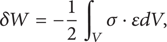
where σ represents the internal stresses and ε represents the internal strains, integrated over the whole volume of the structure, V. The direction of this work is opposed to that of the total internal energy, hence the negative sign.

Strain and Stress Based Formulae for the Elastic Energy in a Beam. E and G are material properties, that is, Young's modulus and the shear modulus or modulus of rigidity, respectively. A, I, and J are the geometric constants of the beam element's section: its area, moment of inertia, and moment of torsion. The internal strains are defined in terms of du and dφ. The internal stresses are axial (N), bending (M), shear (S), and torsional (T):

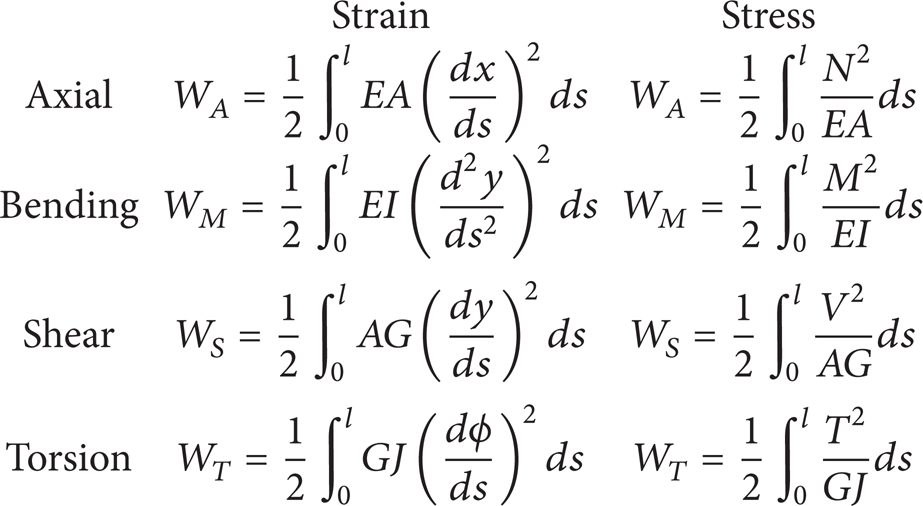
\begin{matrix} Strain & Stress \\ Axial & W_{A} = \frac{1}{2} \int_{0}^{l} E A {(\frac{d x}{d s})}^{2} d s & W_{A} = \frac{1}{2} \int_{0}^{l} \frac{N^{2}}{E A} d s \\ Bending & W_{M} = \frac{1}{2} \int_{0}^{l} E I {(\frac{d^{2} y}{d s^{2}})}^{2} d s & W_{M} = \frac{1}{2} \int_{0}^{l} \frac{M^{2}}{E I} d s \\ Shear & W_{S} = \frac{1}{2} \int_{0}^{l} A G {(\frac{d y}{d s})}^{2} d s & W_{S} = \frac{1}{2} \int_{0}^{l} \frac{V^{2}}{A G} d s \\ Torsion & W_{T} = \frac{1}{2} \int_{0}^{l} G J {(\frac{d ϕ}{d s})}^{2} d s & W_{T} = \frac{1}{2} \int_{0}^{l} \frac{T^{2}}{G J} d s \end{matrix}

(6)

In order to assimilate the above concepts to a structural system, where several elements are combined and attached in N nodes, it is proposed that a straightforward connection be made between the nodes, acting as atoms or molecules, and the beam elements, taken as bonds between them.

The formulae given in (6), either as a function of the internal beam strains or as a function of the internal stresses, can be used to such effect.

Internal stresses (axial A, bending M, shear S, and torsional T) are commonly available from any general purpose finite element Method software. The stress-based integrals of (6) can then be used in discrete form as a sum through the defined integration stations of each element.

Each beam is subdivided in stations for which the stress data can be retrieved, so that the particular nodal internal energy may be approximated by summing the contributions of half of each connected beam.

By summing the energetic state of all the nodes, the total internal energy of the system is then computed as

δ W = - \overset{N}{\underset{i = 1}{\sum ‍}} \overset{b_{i}}{\underset{j = 1}{\sum ‍}} \frac{1}{2} (W_{A b} + W_{M b} + W_{S b} + W_{T b}),

(7)

where b_i denotes the number of beams attached to the ith node and W_Ab, W_Mb, W_Sb, and W_Tb are the respective internal energies of each beam as calculated from (6).

2.3. Added Heat, δQ

The heat added to a system is directly related to the amount of movement of its particles, which are, in our case, represented by the nodes of the investigated structure. Thus it involves the entropy gained by the system in the process and its temperature:

δ Q = T \cdot d S .

(8)

When dealing with the atomic level, solids are treated as regular lattices of atoms, tied together with bonds which cannot vibrate independently. Among many others, this was one of the contributions of Einstein to our current understanding of matter and, probably, the seed of statistical mechanics [18].

In order to account for the energy associated with the movement of these atoms, the vibrations take the form of collective modes which propagate through the material. Such propagating lattice vibrations can be considered to be sound waves, whose speed is the speed of sound in the material. The average of this energy is characterized by the temperature, T, while dS, the increase in entropy, parameterizes the “quality” of such energy, that is, its degree of order.

For our purposes, however, it is not straightforward to make a definition of “structural temperature” and in order to compute the value of the heat change we simply proceed to substitute the values of dU and δW previously obtained through (2) and (7), yielding

δ Q = d U + δ W .

(9)

2.4. Entropy Change, dS

Another term involved in (8) is entropy, S. Traditionally, it is considered to be an intrinsic property of a system. However, recently some authors have claimed that it could be more correct to understand it as a property of the description of the system [6]. From this point of view, and taking into account the many available definitions of entropy, we decided in favour of an interpretation which is closer to the approach provided in thermodynamics.

In order to compute the increase of entropy dS a frequency-based approach was adopted for the computation of the probabilities [19 –21].

First, each of the N nodal internal energies δW_i was calculated for each node, as defined previously in the point B.

Then a constant sized bin histogram representing the nodal energetic states could be created for each model out of a number of simulations sufficiently large. As an illustrative example, Figure 2 shows the histogram corresponding to model A, which is further described in the next section of this paper.

The discrete probability of a node to be in an energy state δW_i is then defined as

p_{i discr} = \frac{freq (δ W_{i})}{N_{tot}},

(10)

where N_tot is the number of nodes of the structure, N, multiplied by the number of simulations (for our example we used 1000). In statistical terms, this value of probability is just the frequency with which the value δW_i is found in a population of N_tot nodal energy states, normalized to the total number of nodal energy states of the model.

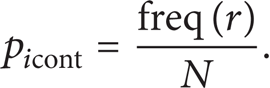
Already in the case of 1000 simulations it is possible to observe the long-tail behaviour of the distribution (Figure 1). In our case this distribution is best approximated by the well-known Pareto law. In Figure 3 the probability mass functions for the same example model A has been plotted with a superimposed Pareto law as explained in [21], which can be described by the equation:

freq (r) = \frac{\ln (1 + (1 / r))}{\ln (R + 1)},

(11)

where r is an integer value between 1 and R, the total number of bins between the largest and the smallest value of nodal energy for all the simulations. With this expression of the frequency it is now possible to recalculate, for each nodal state, the corresponding continuous probabilistic value as

p_{i cont} = \frac{freq (r)}{N} .

(12)

The probabilities can then be obtained for each node after each simulation iteration.

Figure 1:

Histogram for one of the studied models with the frequency of energy states of all the nodes after 1000 simulations. The lowest group of values gets the most of occurrences.

Figure 2:

Probability mass function and Pareto probability density function of nodal energy states for one the studied models. The PMF is obtained by normalization of the frequency. The PDF is approximated as a long-tail Pareto law.

Figure 3:

Underlying nodal distribution for all specimens. Our experiment will evidence how the different topological relationships between the nodes give place to different entropic and energetic behaviours.

Using the node's energy state from the density function of the fitted Pareto distribution, it was then possible to retrieve the continuous value of probability, p_icont.

The increase in entropy was then computed as the sum of all the particular approximated probabilities of each node, times their logarithm:

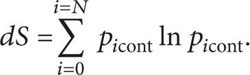
d S = \overset{i = N}{\underset{i = 0}{\sum ‍}} p_{i cont} \ln p_{i cont} .

(13)

The value of the entropy given in (13) provides us with a measure of how much a particular configuration of a structural system under applied forces affects its capacity to absorb heat. It increases linearly with the number of nodes of the structure, N, and is related to the existence of disparities in the distribution of the internal strain energy.

The omission of Boltzmann's constant, k_b, in the definition of (13) must be noted here. This happens as a consequence of the low number of entities involved, far below Avogadro's number, which makes the bulk scaling unnecessary. This also renders our definition of entropy dimensionless, as it is only a function of probabilities.

2.5. Temperature, T

The remaining quantity involved in the description of a system's internal agitation is the temperature. This quantity must not be mistaken with that of ambient temperature or atmospheric temperature but be understood as a reference for the average energy gained by the nodes when subject to displacement.

In our case this value is not available as given data, and its definition for structural systems is not straightforward. However, it is easy to calculate from the definition given by classical thermodynamics in (8):

T = \frac{δ Q}{d S} .

(14)

This value of temperature can be understood as a measure of the tendency of a structural system to dissipate applied energy by displacement instead of concentrating it internally.

Some authors define it as a measure of the quality of a state of a system [22], while others refer to it as the degree of “hotness” of a system [23]. In our case, higher values of temperature imply global deterioration of the static behaviour, whereas at lower values the system shows a higher degree of stiffness.

As follows from (14) and the fact that our definition of entropy has no dimensions, its units are those of energy.

2.6. The Kinetic Energy of a System, KE

Our simulations represent quasistatic processes, where changes are homogeneous throughout the system and slow enough as to maintain a constant state of equilibrium. In these terms, a kinetic definition makes little sense because the process is more commonly defined as simply static.

However, the contribution of the mass of the system to its displaced configuration cannot be neglected.

In general, from the available data of a static simulation, using a general-purpose finite element application, it is possible to derive the following expression for the computation of the kinetic term:

KE = \frac{1}{2} {\{\dot{x}\}}^{T} \cdot [M] \cdot \{\dot{x}\},

(15)

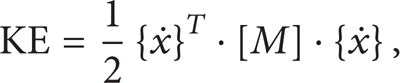
where the superscript dot denotes derivative with respect to time and the mass matrix [M] is assembled by simple addition of each beam elements’ particular masses to their concurrent nodes (i.e., lumped mass matrix).

In our case, however, this expression presents two problems.

We are lacking an objective definition of time.

The quasistatic approach implies that the inertia forces and kinetic energy, respectively, are neglected in the equations of motion and energy balance.

Conveniently, however, a unitary time step can be defined for every iteration of our experiments, yielding

\{\dot{x}\} = \frac{d \{x (t)\}}{d t} = \frac{d \{x (t)\}}{1} = \{x\},

(16)

which means that we can dismiss the time dependency of the structural response and obtain information purely related to the inertia of the system and its resistance to change in its motion. With this simplification it is now possible to rewrite the quasistatic equation for kinetic energy:

K E_{qs} = \frac{1}{2} {\{x\}}^{T} \cdot [M] \cdot \{x\} .

(17)

3. A Practical Example: Numerical Experiments with Conventional Structures

Since the mid-70s many researchers have claimed that input energy can be a good parameter to be considered in seismic design of buildings, given the shortcomings experienced by strength-based seismic design codes [7, 8].

The amount of energy absorbed by a structure during a seismic event, strong enough to induce a certain amount of nonlinear deformation, has been accepted by many researchers as a potentially useful seismic performance indicator [24].

This indicator, however, is difficult to measure in a global sense with the current analysis tools given the methodological limitations mentioned in the introduction of the previous section.

Within our proposed frame, however, a global set of energy-based parameters is straightforward and clear. We will present their relationship to the applied force in a series of quasistatic simulations.

3.1. Description of the Models

Four different specimens were tested, as well as the thermodynamic quantities mentioned earlier computed using a general purpose finite element application. Their configurations were adopted from the seismic regulation Eurocode 8, where a behaviour factor q is defined for several different kinds of structural arrangements. This behaviour factor serves, in a simplified calculation of the nonlinear dynamic response of a structure, to reduce the value of the applied design forces.

Higher values of this factor imply the assumption of better behaviour in the event of plastification of the elements. In other words, the behaviour factor accounts for the ability of the structure to dissipate energy by nonlinear behaviour of rotational springs.

As these are illustrative examples, we have avoided excessive complexity as much as possible. The specimens were treated as 2D models and time-history analysis was not performed. Geometrical and material nonlinear behaviours, however, had to be observed for the sake of completeness.

In Figure 3 the underlying nodal distribution is shown for all four specimens. It can be seen how, sharing all the nodes identical geometric disposition, the particular characteristics of the structural system reside mainly in the topological relationships.

For the modelization of the Timoshenko beam elements, a type of profile common in engineering practice was chosen, with values similar to those corresponding to a 150 × 150 × 10 mm hollow extruded steel bar. The material and section properties are shown in Table 1.

Table 1:

Properties of the beam elements composing the specimens.

Parameter	Value

Number of nodes, N	47
Area (cm²)	56
Modulus of inertia (cm⁴)	1839
Modulus of elasticity (kN/cm²)	21000
Shear modulus (kN/cm²)	8076.92
Material density (kN/cm³)	7.892E–8

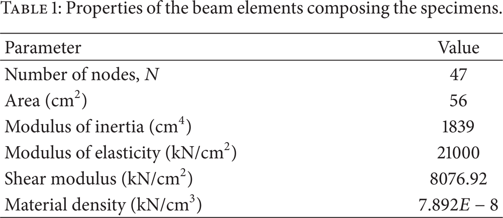
The geometric configuration of each model is displayed in Figure 4, and the nonlinear characteristics of the material employed are depicted in Figure 5.

Figure 4:

Schematic distribution of the nodes and beams which were the subject of the study. The behaviour of each model varies with the disposition of the braces as described in the seismic regulation Eurocode 8.

Figure 5:

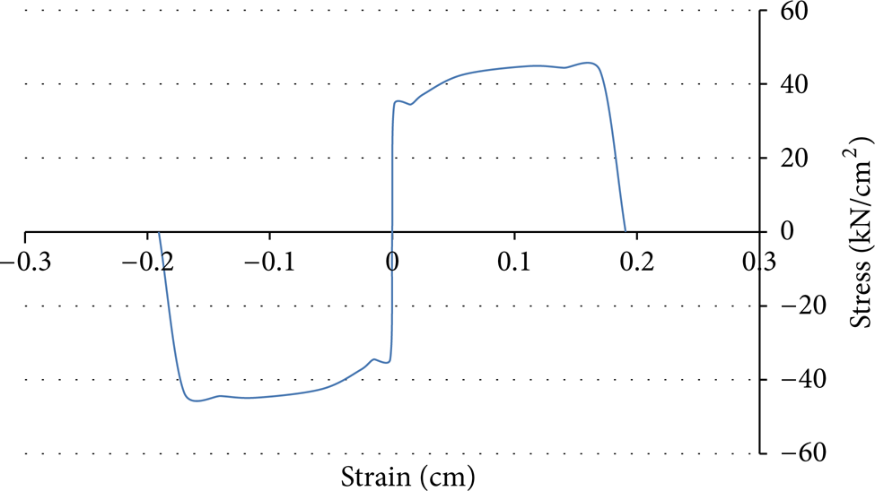
Stress-strain curve of the utilized material (steel). The nonlinear material as well as geometrical behaviour was taken into account in the experiments.

Some characteristic properties of the sample models, such as volume, mass, and moments of inertia are provided in Table 2. Mass was obtained as the product of the volume and the material density (structural steel).

Table 2:

Global properties of the studied specimens.

Parameter	Model A	Model B	Model C	Model D

Volume (cm³)	500256	1078080	857808	833328
Mass (kNs²/cm)	0.0392	0.0798	0.0672	0.0653
Inertia XZ (kN cm's²)	5866	48235	33735	31916
EC 8 Behaviour factor, q()*	5	4	2, 5	5

The total volume of each specimen was computed by multiplying the section area given in Table 1 by the added length of every beam.

The inertia of an assembly of masses is given by the expression:

I = \overset{N}{\underset{i = 1}{\sum ‍}} m_{i} r_{i}^{2},

(18)

where m_i is the lumped mass of each node and r_i is the distance of the node to the centre of gravity of the system. For the computation of the values of inertia only the XZ plane was of interest.

The value of the applied force F was randomly modified around an initial value F_o by means of an exponential function:

F_{t} = F_{o} \cdot e^{- ρ \cdot α / F_{o}},

(19)

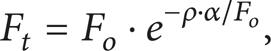
where ρ is a random value between 0 and 1 and α is a control parameter that was fixed as being equal to 5. This leads to a random oscillation of the value of F_t, when F_o = 150 N, between 0 N and 150 N.

The choice of a random function for the definition of F_t was based on the practical advantage of the Monte Carlo method for the exploration of larger search spaces more efficiently.

3.2. Numerical Results and Analysis

Figures 6 to 13 show the relationships of the parameters described in the previous chapter.

Figure 6:

Variation of internal elastic energy with respect to total applied energy. Robust configurations have a short span of values in the horizontal axis as they are opposed to changes in total energy dU.

In Figure 6 the internal elastic potential energy dW is compared to the total applied energy, dU. For all the models the ratio between dW and dU is a constant while no plastic hinges are formed.

The higher flexibility of model A is evidenced by its significant larger span of dissipated energy in comparison with the other three models, which represent a small dot at the beginning of the curve.

Moreover, model A is the only one that actually develops plastic hinges under the same range of applied loads. It is very interesting to observe how the evolution of the global ratio dU/dW evolves in a quadratic fashion, while for the other models it remains within a linear relationship.

Once plastic hinges begin to appear (around the value of 2000 kNcm), the total energy dU increases faster than the change of the internal work, evidencing no further storage of strain energy in the nodes and yet more in the form of displacement.

The last segment of the curve presents a discontinuity originated in the loss of convergence of the nonlinear computations.

The ratio between these two quantities permits comparing how much energy a particular structural configuration is able to absorb with respect to the others. It also allows for the prediction of the behaviour within the elastic range, as it proves that a linear relationship exists between them.

To help understanding the dU quantity, Figure 7 illustrates how the increment of total internal energy of a structural system is only inversely proportional to its stiffness while quadratically dependent on the applied force.

Figure 7:

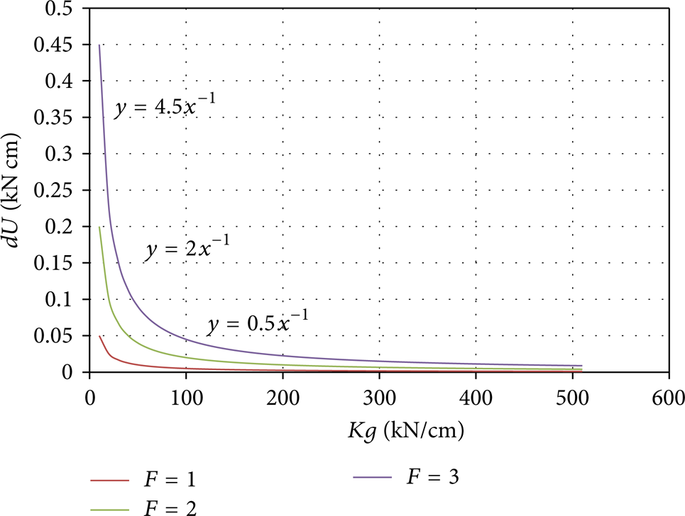
Total internal energy versus the stiffness of a system with a single element. This quantity is a quadratic function of the applied force and varies inversely proportional to the stiffness.

In consequence, flexible structures are capable of dissipating a large amount of applied energy in the form of displacements.

If such systems are only slightly more rigid, however, their dissipative capacity is rapidly reduced and must resource to other mechanisms in order to balance the energies. How these mechanisms basically consist on reducing their entropy will be seen.

Figure 8 depicts the quadratic relationship between the applied load and the total internal energy. Models A and D, with identical values of the coefficient q, have very different responses to the applied force, whereas B and C, which are distant in the value of this parameter, behave very similarly. There is, however, an apparent correlation between the magnitude of the q factor and the slope of the curve: the higher the factor, the higher the slope.

Figure 8:

Variation of internal elastic energy with respect to applied force. The variation of total energy in the system increases quadratically with the applied force.

Figure 9 shows variation of entropy with respect to applied force. The curves present a very interesting parallel decreasing behaviour, indicating that a rise in the energy in the system leads to a reduction of its entropy.

Figure 9:

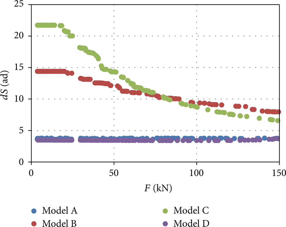
Variation of entropy with respect to the force applied to the system. A higher force results in a higher total energy dU. As dU increases, the individual nodal energies reach higher values, whose probabilities are lower according to the Pareto law. This leads to lower values of the entropy.

Models A and D present very little change in their entropic behaviour, whereas B and C remain stationary until a certain level of force is applied.

This can be explained mathematically, as for lower energy states of the system, the individual probabilities of each nodal state are higher, making the distribution more homogeneous, which leads to a higher entropy.

When the available energy is higher for all the nodes, these must also increase their energetic state and the difference in probabilities from one another increases. This causes the entropy to decrease as, from the definition given in (13), the maximum value of the entropy is achieved for a system in which all the nodes share the available energy equally and are equally probable.

This maximum can be observed in the upper section of each curve, where flat behaviour is present.

In a case of much disparity and the predominance of high values of nodal energy, the entropy tends to a minimum as the majority of the nodes have high values of energy whose probability is lower according to the Pareto law.

Structurally, it provides information about the degree of evenness in the distribution of the internal work, which is directly related to the internal distribution of the tensions. A higher value of entropy means a lower likelihood of concentrated tensions. Hence, models B and C can be considered as structures with a good redistribution of internal strain energy, whereas models A and D are poor in this aspect.

In relation to the behaviour factor q, this makes sense as the purpose of such coefficient is to penalize the structures that show no plastic deformation of its members. Hence, models A and D, with lower entropies, are more likely to concentrate tensions (i.e., nodal energies) that might eventually lead to the appearance of hinges.

To better understand our definition of entropy, Figure 10 illustrates the evolution of dS for the different possible values of p_icont. The highest possible value that a node could, in any case, contribute is that of 0,367 units of entropy and that would be so if the value of its probability were 37% regardless of the structural configuration the node would be immersed in.

Figure 10:

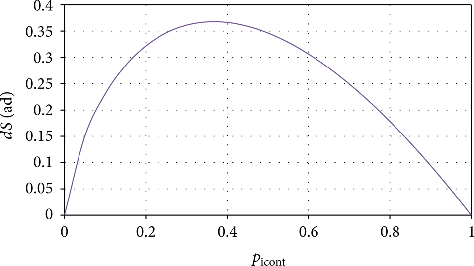
Evolution of the values of entropy with the probability. Higher values of probability do not necessarily imply higher entropy. In fact, the highest entropy of the system would be achieved if the probabilities of all the nodes were in the vicinity of 37%.

For a structural system, this means that unevenly distributed stresses lead to concentrate high values of strain energy at certain points and low in others. According to the Pareto law of Figure 2 this results in a lower value of the global entropy because both high and low nodal energies have, respectively, very low and very high probabilities.

The lowest bottom for the particular configuration of nodes of this study, as represented in Figure 3, corresponds to the lines of models A and D, whose entropy is lowest. These correspond also to the highest values of the behaviour factor q.

The chart shown in Figure 11 is also interesting as it summarizes much of the information provided by both Figures 8 and 9.

Figure 11:

Variation of heat with respect to the force applied to the system. Model A is presented separately given its different scale. The large values of δQ represent big differences between the internal work dW and the total energy, dU.

The value of δQ expresses how close the values of the internal elastic energy dW and the total energy dU are, in other words, how far from unity the ratio γ = δW/dU is.

As it can be appreciated in Figure 8, while in the elastic regime γ is constant regardless of the amount of total energy. For model A, dU is 25% larger than δW, whereas for the rest of models the ratio remains very close to 1.

When plastic dissipative processes are studied, dU and δW depend on each other to a lesser extent. As plastic joints begin to appear, the structure loses stiffness and the possible displacements become larger, so that the value of the kinetic energy is increased.

As a consequence of this, the temperature of the system must also increase. Whereas the entropy of the system remains more or less constant under a constant value of the applied force, the temperature must increase in order to compensate for the larger amount of heat energy available to the system. This principle is the same that explains rubber elasticity.

Keeping in mind the fact that all four models have the same number of nodes, whose topological relationships are dictated by the interconnecting beams, a larger number of connected nodes mean also a more even redistribution of the internal work among them. This explains the difference not only in the response of their internal work but also in the entropy between the models.

The models whose nodes have more connections are both B and C. In the case of model A, any node has at most three beams, whereas for model D the maximum is four.

In the chart of Figure 12 the values of quasistatic kinetic energy are presented against the applied force.

Figure 12:

Variation of quasistatic kinetic energy with respect to force applied on the system. The relationship between kinetic energy and applied force is quadratic. Flexible structures present narrow parabolas.

Figure 13:

Quasistatic kinetic energy versus the mass of a structural system consisting of a single element. The kinetic energy defined here is a quadratic function of the applied force and varies inversely proportional to the mass. The equivalence to the plotted lines in Figure 1 is worth noting, as both dU and KE_qs are quadratic functions of the displacement.

The kind of information that can be extracted from the values of KE_sq is related to whether a structure's behaviour is dominated by the mass of its elements or by their beams’ distribution.

In Figure 13 the quasistatic kinetic energy of a single-beam structure is presented against its mass to illustrate their relationship.

As what occurred in Figure 7 with the stiffness Kg and the total energy dU, this relationship is inversely proportional to the displacement and quadratically dependent on the applied force. This means that a structure with half of the mass of another tends to have much higher values of kinetic energy than if it is only slightly lighter.

As can be seen in Table 2, model A (the lightest) has a mass almost 50% that of model B, which is the heaviest. Models C and D have very similar mass and they are around 80% as heavy as B. Nevertheless, models B and C present a much more similar behaviour in their quasistatic kinetic energies.

Again, for relatively small differences in mass, the influence of the entropy has more importance than the effect of the structural inertial forces.

Figure 14 shows a plot of the temperature against kinetic energy for all four models. Here it is possible to observe the linear dependence between these two variables although they were computed from mathematically independent relationships. This is in accordance with the thermodynamic kinetic theory, by means of which temperature is a parameter in relation to the movement of the particles of a system.

Figure 14:

Temperature versus kinetic energy. Temperature and the quasistatic kinetic energy are linearly related.

Unfortunately, in this study a numerical correlation between the two quantities was not found. It would be more correct to search this correlation within the context of time-history analysis, where also velocities and accelerations could be taken into account. Nevertheless, this is a very promising result that encourages further research.

In Figure 15, the deformed shapes of the four structures are shown for comparison. How model D “activates” the rotational degrees of freedom of extra nodes can be seen, increasing its internal energy. This explains how this model can create points of high concentration of stresses, hence reducing its entropy. Similarly, model A also presents rotated beams whereas in models B and C these remain straight.

Figure 15:

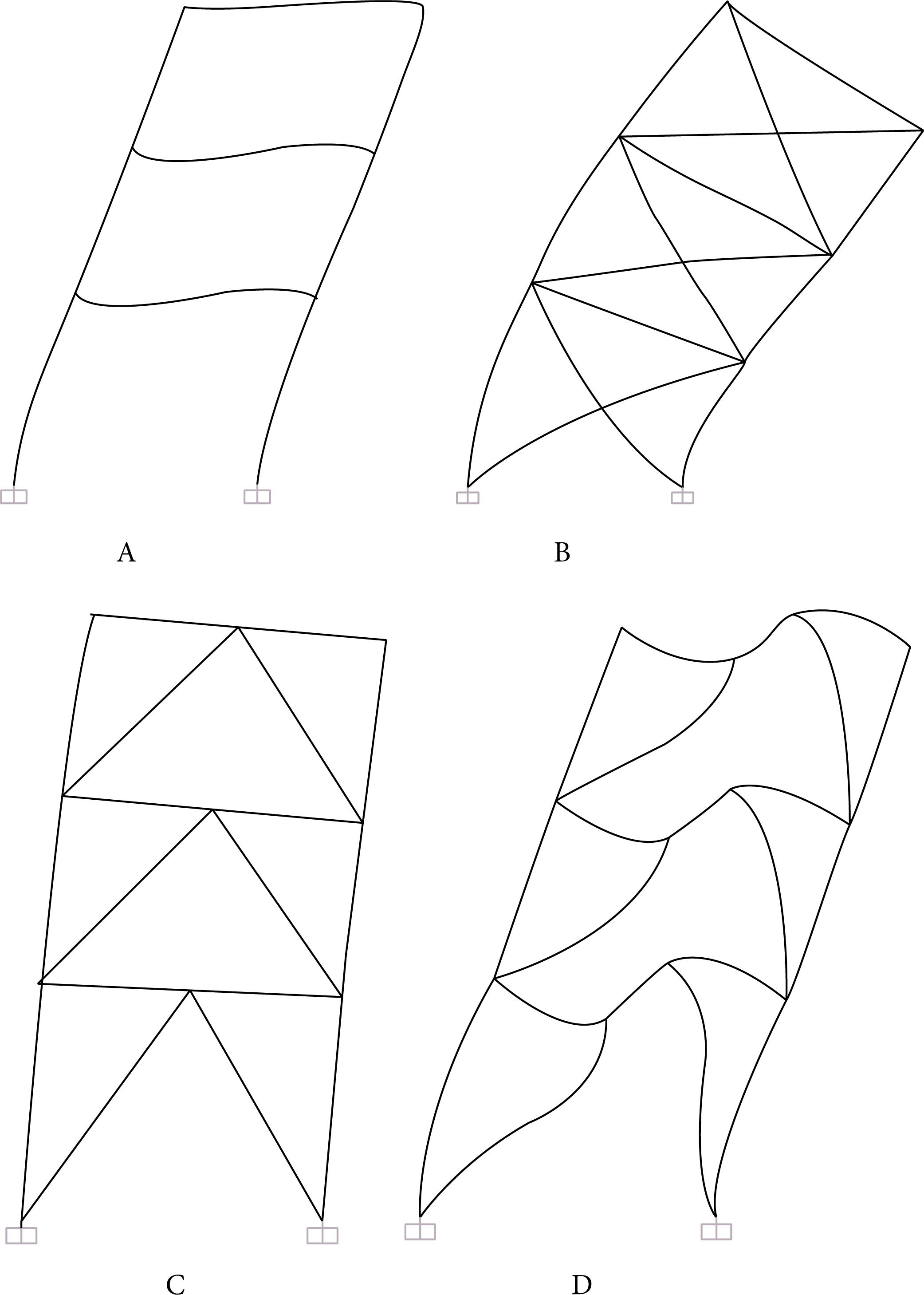
The deformed shapes of the models under the applied load. Model A was magnified by a factor of 1000, whereas models B, C, and D were magnified by a factor of 10000.

4. Discussion and Future Work

In the present work a series of quantities from statistical mechanics have been defined to describe and compare the properties of a set of structures. The values of these quantities were obtained by assimilating certain structural systems to an aggregate of interconnected nodes undergoing a quasistatic process of thermodynamic change. In this manner, it was possible to define

the number of nodes, N, corresponding to the size of the assembled matrices,

the internal energy, dU, as the amount of work done by the external forces on the structural system,

the internal strain energy, δW, as the amount of such work mechanically stored in the nodes,

the added heat, δQ, as the energy dissipated in the form of displacements,

the change in entropy, dS, as a measure of the degree to which δW is evenly distributed throughout the nodes,

the temperature, T, as the ratio between the added heat and the entropy,

the internal quasistatic kinetic energy, KE_qs, as a measure of the influence of the mass of the system.

These properties have been identified in a group of four structural configurations adopted from the seismic regulation Eurocode 8. The choice of a structural engineering reference provides our framework with a sound background for the establishing of comparisons and, more importantly, a handy factor, q, which is called a “behaviour factor.”

There seems to be a possibility of characterizing this empirical factor in a more rigorous manner by means of the definition of a value of entropy for each structural configuration.

We have also presented a novel application of entropy in order to define the degree to which internal energy is evenly distributed within a structure. Uniform distribution of this energy, being dependent on internal stresses, means a lower likelihood of encountering overstressed points while underutilizing others. Structures with high values of entropy are less likely to present local failures and will do so only after resourcing all of its available elements.

From our experiments, more flexibility also means lower entropy. However, a more flexible structure can also respond to a much wider range of applied energies. It is the trade-off between material economy, energetic capacity, and entropy which makes a good structural design.

It was concluded that the techniques developed for analyzing systems from the point of view of statistical mechanics work very well with structural systems.

Within the framework presented in this paper, it is possible to determine whether a structural system will require from its elements the ability to store applied energy or to deform in order to dissipate it, and to what extent.

This work opens up the possibility of some additional interactions, such as

the study of applications to real built structures,

the application to algorithms for the study of nonlinear behaviours,

the extension of the simulations to time-history analysis for the characterization of a term of “structural temperature,”

the research in the characterization of the externally applied loads as sources of energy, so that the whole system can be treated as an energetic exchange process,

experimentation with different laws for the fitting of the probabilities in order to see how they affect the computation of entropy,

the possibility of combining together the defined parameters with optimization techniques; their straightforward identification with qualitative properties makes them ideal candidates as design target variables,

the extension to different types of finite elements other than Timoshenko beams.

Conflict of Interests

The authors declare that there is no conflict of interests regarding the publication of this paper. All the research presented here has been conducted in a completely independent manner with the sole aid and resources of the academic institutions listed in the header of the work.

References

Wunderlich

and Pilkey

W. D.

, Mechanics of Structures: Variational and Computational Methods, CRC Press, Boca Raton, Fla, USA, 2003.

Reddy

J. N.

, Energy Principles and Variational Methods in Applied Mechanics, John Wiley & Sons, 2002.

Piperno

and Farhat

, “Partitioned procedures for the transient solution of coupled aeroelastic problems, part II: energy transfer analysis and three-dimensional applications,” Computer Methods in Applied Mechanics and Engineering, vol. 190, no. 24–25, pp. 3147–3170, 2001.

Jacob

G. C.

Fellers

J. F.

Simunovic

, and Starbuck

J. M.

, “Energy absorption in polymer composites for automotive crashworthiness,” Journal of Composite Materials, vol. 36, no. 7, pp. 813–850, 2002.

Marsden

J. E.

and West

, “Discrete mechanics and variational integrators,” Acta Numerica, pp. 1–158, 2001.

Housner

G. W.

, “Limit design of structures to resist earthquakes,” in Proceedings of the 1st World Conference on Earthquake Engineering vol. 5, pp. 1–13, Berkeley, Calif, USA, 1956.

Khashaee

Mohraz

Sadek

Lew

H. S.

, and Gross

J. L.

, Distribution of Earthquake Input Energy in Structures, Building and Fire Research Laboratory, National Institute of Standards and Technology, Gaithersburg, Md, USA, 2003.

Manfredi

, “Evaluation of seismic energy demand,” Earthquake Engineering & Structural Dynamics, vol. 30, no. 4, pp. 485–499, 2001.

Tohei

Kuwabara

Oba

, and Tanaka

, “Debye temperature and stiffness of carbon and boron nitride polymorphs from first principles calculations,” Physical Review B, vol. 73, no. 6, Article ID 064304, 2006.

10.

Cherian

and Mahadevan

, “Elastic properties of carbon nanotubes: an atomistic approach,” Journal of Nanoscience and Nanotechnology, vol. 7, no. 6, pp. 1779–1782, 2007.

11.

, Entropic elasticity of polymers and their networks [Ph.D. thesis], University of Pennsylvania, 2011.

12.

Liu

Huang

Jiang

, and Hwang

K. C.

, “The atomic-scale finite element method,” Computer Methods in Applied Mechanics and Engineering, vol. 193, no. 17–20, pp. 1849–1864, 2004.

13.

Niven

R. K.

, “Non-Asymptotic thermodynamic ensembles,” Europhysics Letters, vol. 86, no. 2, 2009.

14.

Niven

R. K.

, “Combinatorial entropies and statistics,” The European Physical Journal B, vol. 70, no. 1, pp. 49–63, 2009.

15.

European Committee for Standardization, Eurocode 8: Design of Structures for Earthquake Resistance, European Committee for Standardization, 2004.

16.

Nahas

M. N.

and Abd-Rabou

, “Finite element modeling of carbon nanotubes,” International Journal of Mechanical and Mechanics Engineering, vol. 10, no. 3, pp. 19–24, 2010.

17.

Landau

L. D.

and Lifshitz

E. M.

, Theory of Elasticity, vol. 7 of Course of Theoretical Physics, Heinemann, Malaysia, 1986.

18.

Moore

T. A.

and Schroeder

D. V.

, “A different approach to introducing statistical mechanics,” American Journal of Physics, vol. 65, no. 1, pp. 26–36, 1997.

19.

Alexandrowicz

, “Entropy calculated from the frequency of states of individual particles,” Journal of Statistical Physics, vol. 14, no. 1, pp. 1–9, 1976.

20.

Knuth

K. H.

, “Optimal data-based binning for histograms,” Cornell University Library, Submitted, http://arxiv.org/abs/physics/0605197.

21.

Kafri

, “The distributions in nature and entropy principle,” Computer Research Repository, http://arxiv.org/abs/0907.4852.

22.

Bryan

G. H.

, Thermodynamics: An Introductory Treatise Dealing Mainly with First Principles and Their Direct Applications, B.G. Teubner, 1907.

23.

Mareš

J. J.

, “Hotness manifold, phenomenological temperature and other related concepts of thermal physics,” in Glassy, Amorphous and Nano-Crystalline Materials, pp. 327–346, Springer, Amsterdam, The Netherlands, 2011.

24.

Hosseini

and Vaseghinia

M. A.

, “A new insight to the earthquake input energy and its variation with building's dynamical characteristics,” in Proceedings of the the 14th World Conference on Earthquake Engineering, Beijing, China, 2008.