Sage Journals: Discover world-class research

Abstract

Reducing friction resistance and aerodynamic heating has important engineering significance to improve the performances of super/hypersonic aircraft, so the purpose of transition control and turbulent drag reduction becomes one of the cutting edges in turbulence research. In order to investigate the influences of wall cooling and suction on the transition process and fully developed turbulence, the large eddy simulation of spatially evolving supersonic boundary layer transition over a flat-plate with freestream Mach number 4.5 at different wall temperature and suction intensity is performed in the present work. It is found that the wall cooling and suction are capable of changing the mean velocity profile within the boundary layer and improving the stability of the flow field, thus delaying the onset of the spatial transition process. The transition control will become more effective as the wall temperature decreases, while there is an optimal wall suction intensity under the given conditions. Moreover, the development of large-scale coherent structures can be suppressed effectively via wall cooling, but wall suction has no influence.

1. Introduction

Recently, the development of near space super/hypersonic air-breathing aircraft has become a hot research topic in aerospace technology. The transition process from laminar flow to turbulence exists widely in the super/hypersonic aircraft boundary layers, resulting in a sharp increase in the friction resistance and heat flux. Therefore, it would have important engineering significance for super/hypersonic aircraft design on understanding the mechanisms of the transition, as well as accurately predicting and controlling the transition.

Due to the development of computational fluid dynamics (CFD) and computer technology, numerical simulation has become a more and more important tool for transition research [1 –3]. Large eddy simulation [4] (LES) is developed for the comprehensive consideration of the requirements of engineering applications and the limitations of computational resources, and it is a numerical method between Reynolds-averaged Navier-Stokes equations (RANS) and direct numerical simulation (DNS). Compared with RANS on the one hand, the subgrid-scale model can be universal and provide the true information of instantaneous flow field, indicating that LES can be applied to predict the separation, transition, and other complex flow phenomena. By comparing it with DNS, on the other hand, LES can save considerable computational resources and be adaptable to high Mach number and Reynolds number flows. Currently, LES has been successfully applied to the numerical simulation of boundary layer transition [5 –9] and had positive effects on the mechanism study of transition.

A distinctly practical motivation for transition research is the desire to effectively control the process from laminar flow to turbulence. Depending on the circumstances, the effects of transition control can be divided into two aspects. One is to promote transition, such as promoting the mixing of fuel and air in combustors. On the other hand the other aspect is to delay it, namely, laminar flow control (LFC) technology. For example, in order to reduce the skin friction drag and heat conduction, the boundary layer can be kept as a state of laminar flow through LFC. A review of this field was given by Reshotko [10]. Well-established boundary layer transition control techniques include the application of pressure gradients, wall motion, wall suction or blowing, wall heating or cooling, and the injection of different gases into the boundary layer [11]. These control techniques are based on a stabilization of the mean laminar boundary layer profile. Kleiser and Laurien [12, 13] also realized the direct control of instability waves by superposition of antiphased disturbances. The above methods are active control techniques; in addition, there are passive control techniques. Domaradzki and Metcalfe [14] obtained twice the normal transition Reynolds number through the use of compliant surfaces in boundary layer flow.

Wall cooling and suction are the main techniques for compressible boundary layer transition control. The linear stability theory indicates that wall cooling is expected to be stabilizing for first mode disturbances and destabilizing for second mode disturbances, while wall suction is expected to be stabilizing for both first and second mode disturbances. The stability theory cannot predict the transition, while numerical simulation can obtain the whole transition process. In this paper, the effects of wall cooling and suction on the spatially evolving supersonic flat-plate boundary layer transition and fully developed turbulence at freestream Mach number 4.5 are performed by using LES.

2. Numerical Simulation Method

A massive parallel numerical simulation platform for LES developed by ourselves is used in present work. In this code, the Favre filter is applied to the compressible Navier-Stokes (NS) equations, while the filtered energy equation is represented in terms of Vreman's resolved total energy [15]. The subgrid stress is modeled by a dynamic mixed subgrid-scale (SGS) model [16], which is extended from the combination of compressible Smagorinsky model and scale similarity model. The subgrid heat flux is modeled using the eddy diffusivity model.

The governing equations are approximated by a finite difference method. After the local Steger-Warming flux splitting, the convective terms are discretized with a fifth-order upwind compact difference scheme, which is developed by Fu and Ma [17]. A sixth-order central compact difference scheme developed by Lele [18] is applied to the viscous terms. The time integration is conducted by an explicit third-order Runge-Kutta method [19], which satisfies the TVD property. The parallel computation is implemented based on MPI.

The computational configuration of a flat-plate is shown in Figure 1. The x-, y-, and z-axes are set along the streamwise, wall-normal, and spanwise directions, respectively, and L_x, L_y, and L_z are the size of the computational domain in the corresponding directions. The inflow boundary of the computational domain corresponds to a location x_in from the leading edge of the flat-plate.

Figure 1:

Configuration of a flat-plate flow.

Because of using the spatial mode, the initial flow field of the inflow boundary consists of two parts: one part is the basic mean flow, and the other part is the disturbances which are introduced to make the transition occur. The mean flow is the similarity solution of the compressible laminar boundary layer, while the disturbances consist of a pair of the most unstable oblique first mode disturbances [20]. Periodic boundary condition is imposed on the spanwise direction, and nonslip boundary condition is employed on the flat-plate. In order to effectively implement nonreflecting boundary condition, the fringe method [21] is adopted for the outlet and upper boundary. In this method, a buffer region is added to the boundary of the original computational domain. In order to decay the reflected wave, the artificial dissipation is added to the governing equations in this region.

According to the above method, the spatial transition process over a flat-plate boundary layer at a freestream Mach number of 4.5 and a Reynolds number of 10000 based on freestream velocity u_∞ and inflow displacement thickness δ_d0 has been investigated in [22]. The location x_in is equal to 90.5δ_d0. The wall temperature is chosen to be equal to its laminar adiabatic value. The three-dimensional computational domain consists of 418.88δ_d0 × 7.57δ_d0 × 60δ_d0 (L_x × L_y × L_z). The total number of grid points is 983 × 101 × 33 (x × y × z). The grid spacing is placed uniformly along the spanwise direction and stretched following a hyperbolic tangent law along the wall-normal direction. The grid is uniform along the streamwise direction where x < 430.85δ_d0 and stretched grid is used as a buffer region downstream. The following studies of wall cooling and suction effects are based on this simulation result.

3. Results and Discussion

Because the spanwise direction is periodic, the mean values are obtained by the ensemble averages both in time and in spanwise direction. In the analysis to follow, an angle bracket or an overbar denotes a Reynolds-averaged quantity, and a single prime represents a fluctuation relative to Reynolds average.

3.1. Wall Cooling

In order to investigate the influence of wall cooling, the supersonic flat-plate boundary layer transition processes at three different wall cooling conditions are calculated, and the wall temperatures are shown in Table 1. The subscript “w” represents the dimensionless quantities on the wall. C0 represents the case in [22], while the calculation parameters of case C1 to case C3 are the same as C0 except for the wall temperature. The wall temperature is successively reduced from case C1 to case C3, reflecting the effect of wall cooling enhanced.

Table 1:

Wall cooling parameters.

Case	Wall temperature

C0	T _w
C1	0.9T_w
C2	0.6T_w
C3	0.3T_w

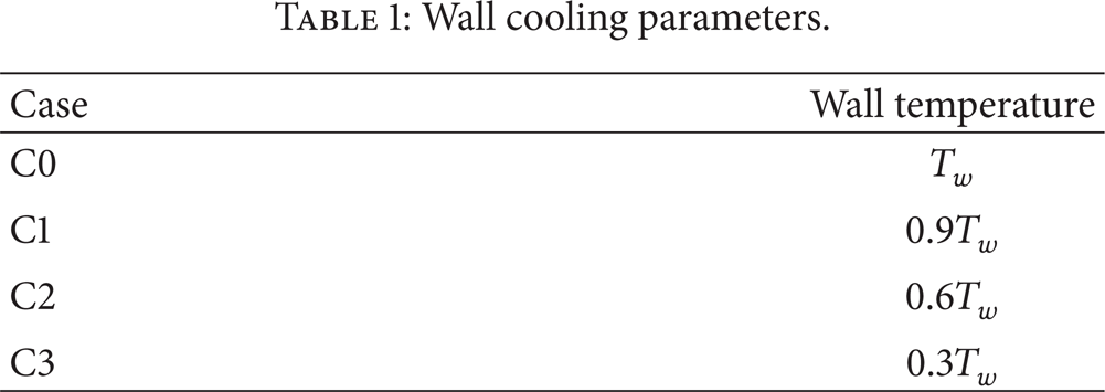
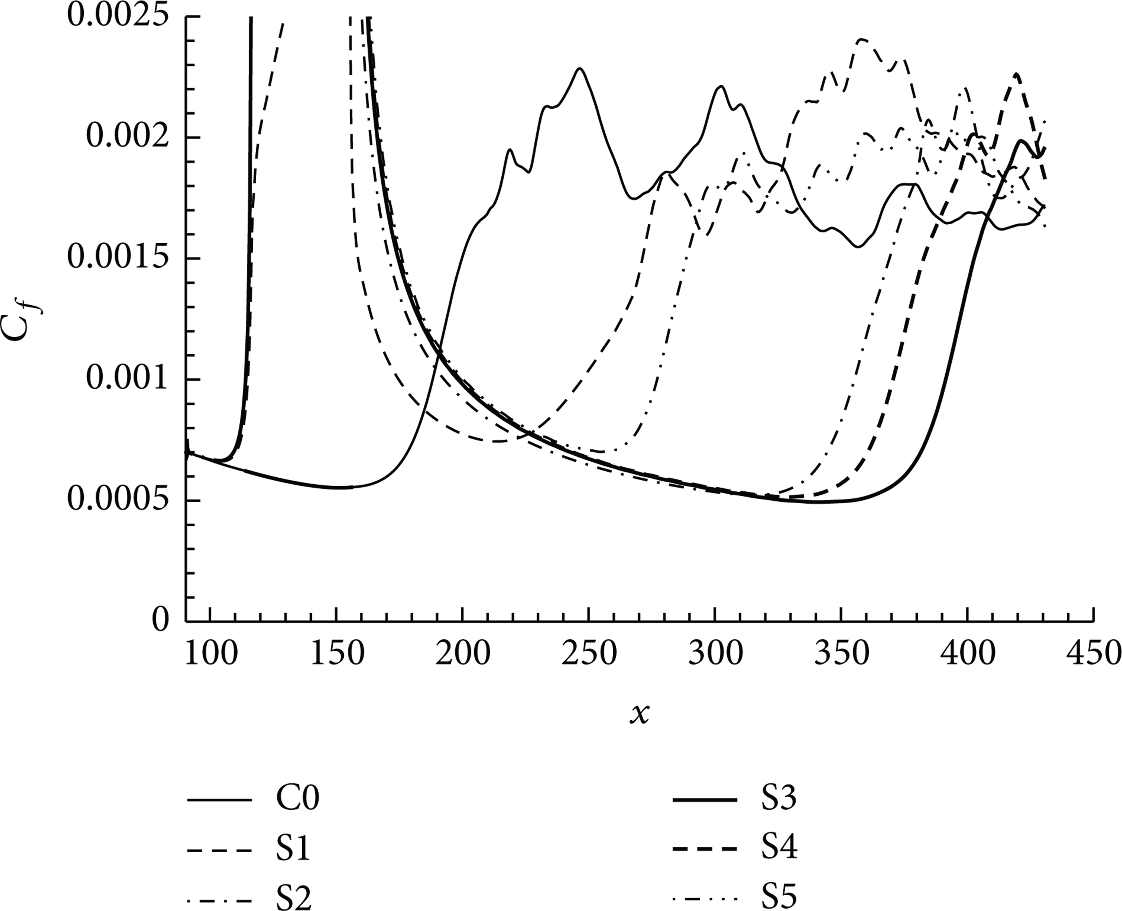
Figure 2 depicts the evolution of the skin friction coefficient C_f along the streamwise direction for all cases, which is defined as

C_{f} = \frac{τ_{w}}{(1 / 2) ρ_{\infty} V_{\infty}^{2}}, τ_{w} = {\bar{μ \frac{\partial u}{\partial y}}|}_{w} .

(1)

It can be seen that the skin friction increases fast at x ≈ 170δ_d0 for C0, and the corresponding transition Reynolds number Re_x is about 1.7 × 10⁶. When the wall temperature drops to 0.9T_w, the skin friction rises up quickly at x ≈ 175δ_d0 for C1, and the corresponding transition Reynolds number is about 1.75 × 10⁶, which increases by 3% compared with C0. As the wall temperature further decreases to 0.6T_w, the transition point and corresponding transition Reynolds number are x ≈ 200δ_d0 and Re_x ≈ 2.0 × 10⁶, respectively, which increases by 18% compared with C0. Furthermore, when the wall temperature is equal to 0.3T_w, the transition point and corresponding transition Reynolds number are x ≈ 290δ_d0 and Re_x ≈ 2.9 × 10⁶, which significantly increases by 70% compared with C0. The above analysis shows that the wall cooling can delay the transition process, and the delayed effectiveness becomes more obvious with decreasing wall temperature, but the transition process is not completely suppressed until the wall temperature reaches 0.3 times the adiabatic wall temperature.

Figure 2:

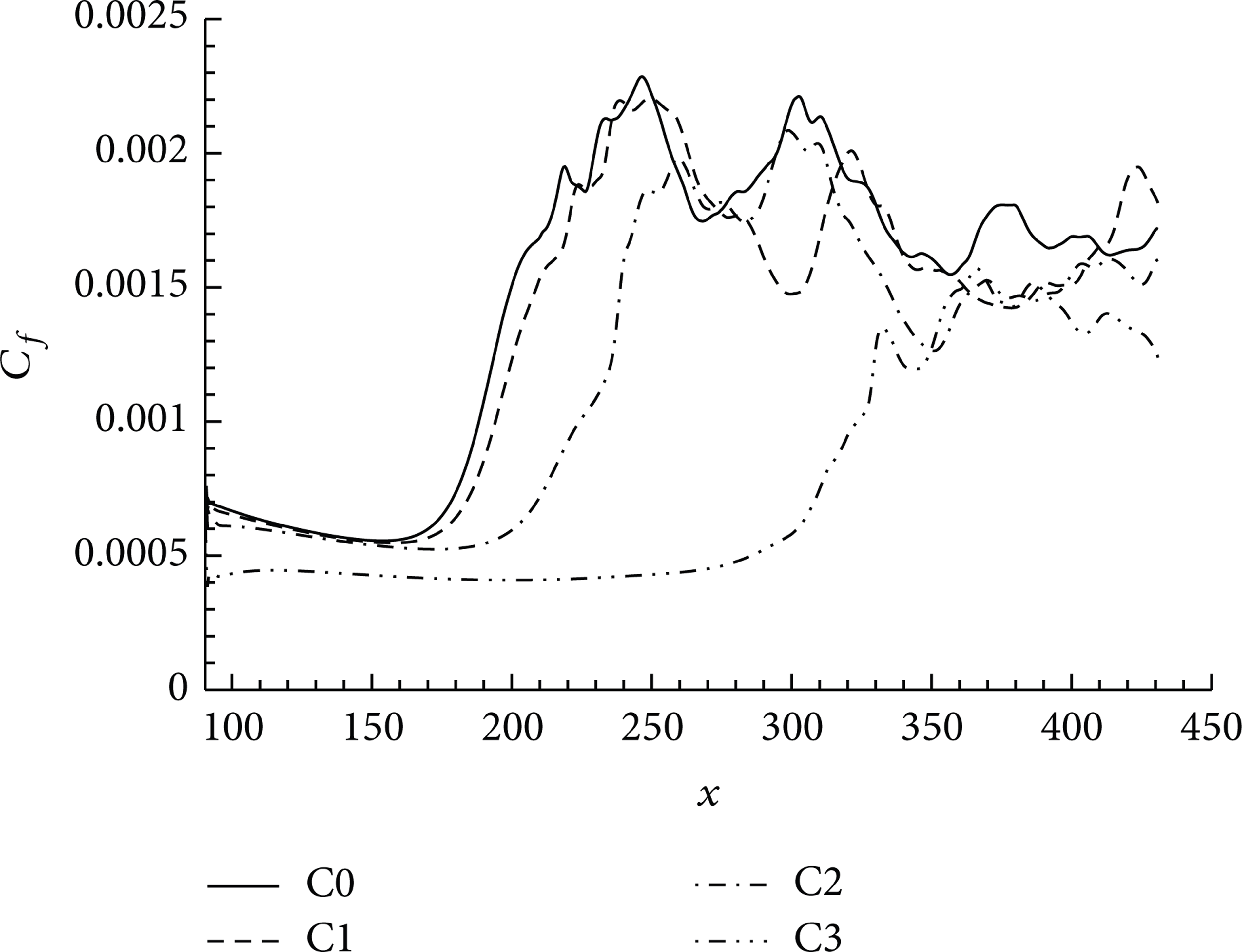
Distributions of the skin friction coefficient with wall cooling.

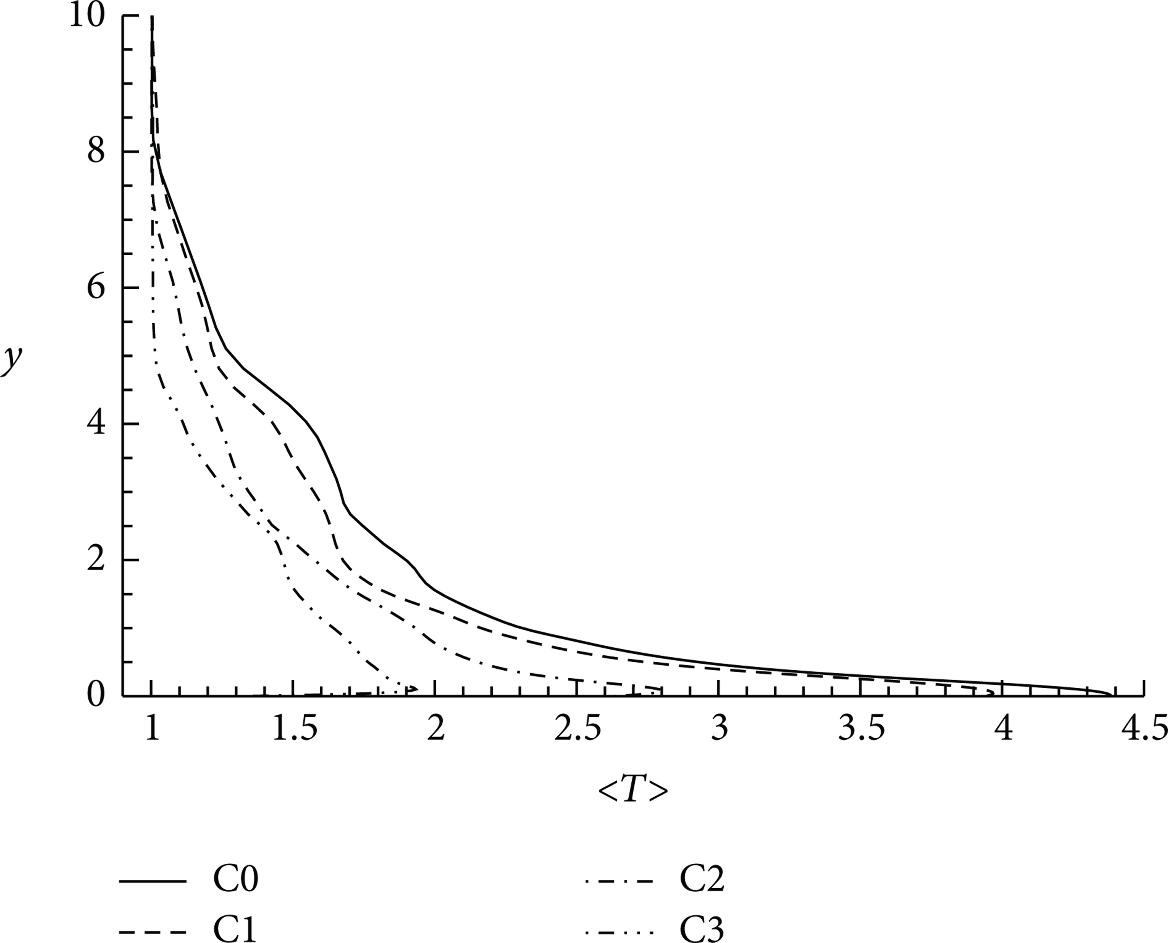
Figure 3 shows the profiles of mean streamwise velocity at four different streamwise locations, including x = 210δ_d0, 246δ_d0, 335δ_d0, and 428δ_d0. The square symbol in Figure 3 represents the laminar velocity profile at the inflow boundary of the computational domain. At x = 210δ_d0, the profiles of C0 and C1 change greatly and inflexion points appear near the critical layer, and the profile of C2 has little change and still maintains laminar flow, while the profile of C3 is almost consistent with the inflow profile. At x = 246δ_d0, the profiles of C0 and C1 still have significant change compared to the previous position, and the profile of C2 also undergoes rapid modification from laminar profile and inflexion points appear, while the profile of C3 has little change and only the boundary layer thickness increases. At x = 335δ_d0, the profiles of C0, C1, and C2 are close to each other and show a typical distribution of turbulent flow, and the profile of C3 significantly deviates from the inflow profile. When x = 428δ_d0, the profiles of all four cases are close to each other, indicating that it has entered the stage of fully developed turbulence. Obviously, the wall cooling changes the mean velocity profiles in the boundary layer and thus increases the stability of the flow field. Figure 4 shows the distributions of mean temperature at x = 400δ_d0, where the transition processes for all cases have been completed and the equilibrium state of fully developed turbulence has been reached. It can be seen that the temperature gradient on the wall gradually increases with decreasing wall temperature; moreover the position of the peak value deviates from the wall.

Figure 3:

Profiles of the mean streamwise velocity with wall cooling. (a) x = 210δ_d0. (b) x = 246δ_d0. (c) x = 335δ_d0. (d) x = 428δ_d0.

Figure 4:

Profiles of the mean temperature with wall cooling (x = 400δ_d0).

For compressible flow, the displacement thickness δ_d and momentum thickness θ are defined as

\begin{matrix} δ_{d} = \int_{0}^{δ} (1 - \frac{ρ u}{ρ_{\infty} u_{\infty}}) d y, \\ θ = \int_{0}^{δ} \frac{ρ u}{ρ_{\infty} u_{\infty}} (1 - \frac{u}{u_{\infty}}) d y . \end{matrix}

(2)

The boundary layer thickness δ is defined as the distance from the wall where the mean velocity reaches 99% of the freestream velocity. The various thicknesses of boundary layer obtained from the present simulation are plotted in Figure 5. It can be seen from Figure 5(a) that the wall cooling makes the boundary layer thickness near the inflow boundary decrease, and the growth rate downstream also reduces (i.e., the slope of the cures decreases). Based on the linear stability theory, a thin boundary layer is less likely to become turbulent. For all cases, the boundary layer thickness rises up quickly when its value reaches about 1.85, indicating that the transition process tends to occur. Because of the wall cooling reducing the boundary layer thickness in the laminar region, the position for rapid increase moves downstream with decreasing wall temperature, indicating again that the wall cooling can delay the transition process. As shown in Figure 5(b), the profiles of displacement thickness exhibit a similar trend to the boundary thickness; thus the overall distribution decreases with decreasing wall temperature. According to Figure 5(c), the wall cooling has little effect on the momentum thickness in the laminar region and only delays its rapid growth.

Figure 5:

Distributions of various thicknesses of boundary layer with wall cooling. (a) Boundary layer thickness. (b) Displacement thickness. (c) Momentum thickness.

As can be seen in Figure 4, the wall cooling reduces the distribution of mean temperature in the boundary layer, so the local average speed of sound $\bar{a}$ also decreases. The turbulent Mach number M_t is defined as

M_{t} = \frac{\sqrt{\bar{u^{' 2} + v^{' 2} + w^{' 2}}}}{\bar{a}} .

(3)

Consequently, the turbulent Mach number will change with wall cooling. The profiles of the turbulent Mach number at x = 400δ_d0 are given in Figure 6. In the viscous sublayer, the turbulent Mach number changes a little. In the buffer and logarithmic region, the distributions of the turbulent Mach number increase significantly with decreasing wall temperature. The peak value of the turbulent Mach number is equal to 0.43 for C0 and increases to 0.68 for C3, indicating that the wall cooling can enhance the compressibility effects. Furthermore, the position of the peak value moves away from the wall. Therefore, the distributions of the turbulent Mach number in the boundary layer are not only depending on freestream Mach number, and the effect of wall cooling is also significant.

Figure 6:

Profiles of the turbulent Mach number with wall cooling (x = 400δ_d0).

The rms density fluctuations normalized by the mean density profile at x = 400δ_d0 are presented in Figure 7. As shown in Figure 7(a), when the abscissa is normalized by conventional wall variables, the values of the rms density fluctuations have no significant differences for all cases; just the overall distribution deviates from the wall. According to Figure 7(b), the profiles of the rms density fluctuations for all cases have similarity when the abscissa is normalized by boundary layer thickness.

Figure 7:

Profiles of the rms density fluctuations with wall cooling (x = 400δ_d0).

Figure 8 depicts the instantaneous isosurface of Q = 0.02 for case C0 to case C3, respectively, where Q is the second invariant of the velocity gradient tensor [23]. These figures show the evolution of complex vortex structures in the transition process. As shown in Figure 8(a), a series of open-tip Λ vortices are observed between 170δ_d0 and 210δ_d0, and these Λ vortices are staggered in the streamwise direction. Starting from x = 210δ_d0, the Λ vortices are stretched and underwent deformation by the shear effect, forming hairpin-like vortices which have close tips and open tails. Subsequently, the hairpin vortices continue to develop into ring-like vortices along the downstream. When x > 250δ_d0, the broken ring-like vortices lead to the generation of some small scale structures, indicating that the transition process tends to finish. It can be found through a comparison that the appearance of the Λ vortices moves downstream with decreasing wall temperature. The structures of Λ vortices, hairpin-like vortices, and ring-like vortices are obvious for case C1. Case C2 has also maintained Λ vortices, but the hairpin-like vortices and ring-like vortices are obscure. Furthermore, the structures of Λ vortices for case C3 also tend to be obscure. Therefore, the wall cooling can suppress the generation and development of the large-scale coherent structures in the transition process.

Figure 8:

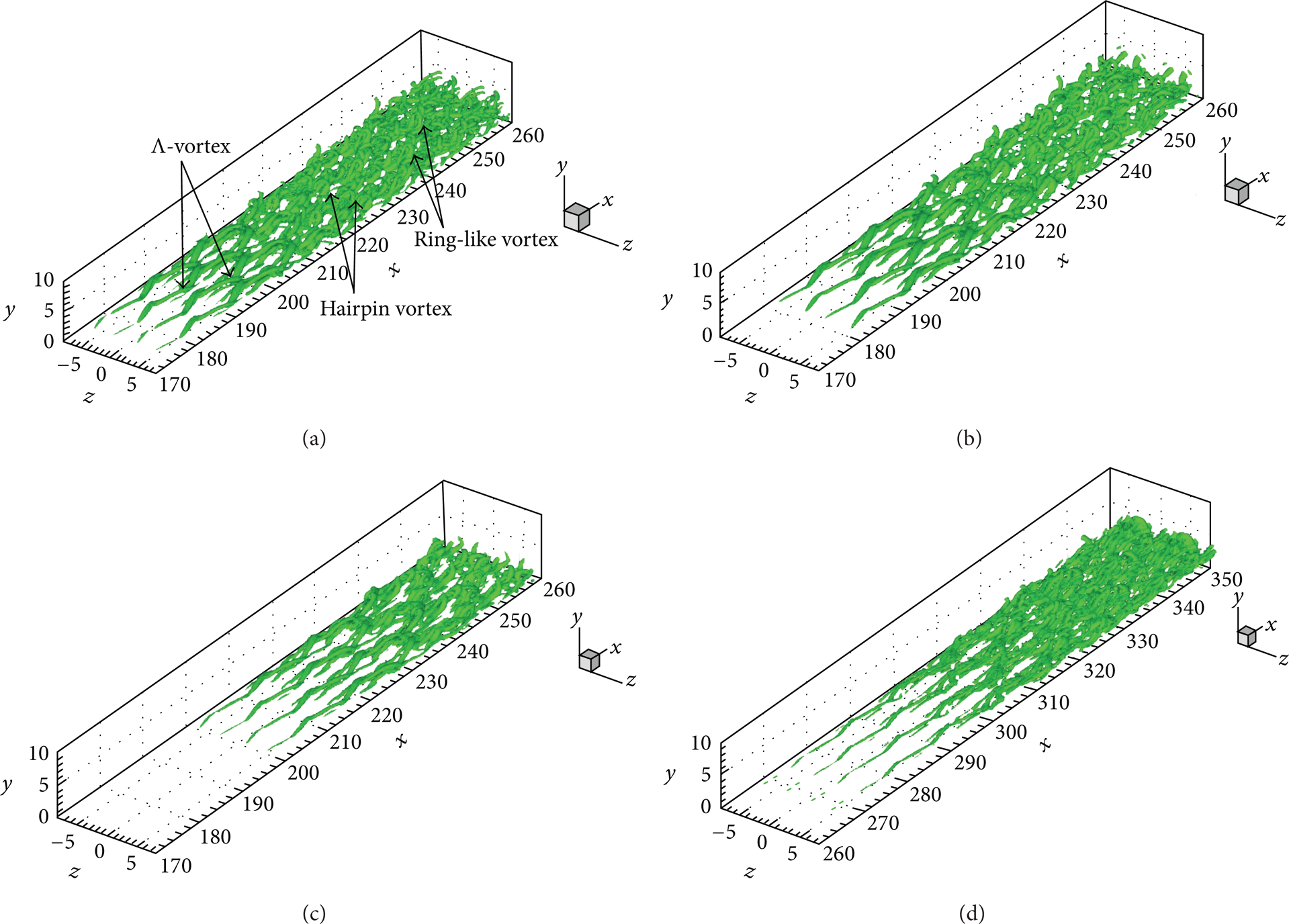
Instantaneous isosurface of Q = 0.02 with wall cooling. (a) C0. (b) C1. (c) C2. (d) C3.

3.2. Wall Suction

The influence of wall suction on supersonic flat-plate boundary layer transition process is investigated in this section. The wall suction parameters are summarized in Table 2. ρ_w and v_w represent the density and wall-normal velocity in the wall suction region. The suction intensity is defined as the ratio of suction flow rate and freestream flow rate per unit area; therefore the suction intensity gradually increases from case S1 to case S5. The wall suction region chosen in present simulation is located between the inflow boundary and transition point of case C0, and the specific streamwise position is 116.69δ_d0 ≤ x ≤ 155.96δ_d0.

Table 2:

Wall suction parameters.

Case	ρ_wv_w/ρ_∞V_∞

C0	0
S1	−2.0 × 10⁻³
S2	−5.0 × 10⁻³
S3	−8.0 × 10⁻³
S4	−9.0 × 10⁻³
S5	−2.0 × 10⁻²

Figure 9 plots the distributions of the skin friction coefficient with wall suction. The bold section of cure C0 represents the wall suction region. It can be seen that the skin friction coefficient in this region increases significantly after adding suction. In order to further understand the wall suction effect on the transition process, Table 3 lists the related parameters of transition point, including the position where transition occurs, the corresponding transition Reynolds number, and the percentage of increase compared with case C0. It can be seen that the transition point gradually moves downstream from S1 to S3 with increasing wall suction intensity, making the transition Reynolds number increase. As the wall suction intensity is equal to −9.0 × 10⁻³, the transition point of S4 moves upstream compared to S3.

Table 3:

Comparison of the transition point parameters.

Case	x_{tr ⁡}/δ_d0	${Re}_{x_{tr}}$	↑%

C0	170	1.7 × 10⁶	0
S1	220	2.2 × 10⁶	29
S2	320	3.2 × 10⁶	88
S3	345	3.45 × 10⁶	103
S4	330	3.3 × 10⁶	94
S5	260	2.6 × 10⁶	53

Figure 9:

Distributions of the skin friction coefficient with wall suction.

When the wall suction intensity significantly increases to −2.0 × 10⁻², the transition Reynolds number of case S5 is less than that of S2 to S4, but still more than C0 and S1. According to the above analysis, the wall suction can also delay the transition process. However, there is an optimal suction intensity under the given conditions, and the delayed effectiveness will be weakened when the suction intensity falls below or exceeds the optimal value.

Figure 10 gives the profiles of mean streamwise velocity with wall suction at four different streamwise locations, involving x = 150δ_d0, 210δ_d0, 335δ_d0, and 428δ_d0. At x = 150δ_d0, applying wall suction makes the boundary layer thickness decrease rapidly, and the velocity gradient near the wall increases significantly, resulting in the skin friction coefficient increases. At x = 210δ_d0, the velocity profiles of all wall suction cases maintain laminar profile and are close to the inflow profile. At x = 335δ_d0, the profiles of S1 and S5 obviously deviate from the laminar profile and are close to the turbulent profile of C0, while that of S2 to S4 remains laminar profile and only the boundary layer thickness increases. At x = 428δ_d0, the profiles of S2 to S4 also deviate from the laminar profile and inflexion points exist but are still not consistent with C0, indicating that the flow field has not yet entered the stage of fully developed turbulence. It can be found that the wall suction also changes the velocity profiles of the mean flow field and tends to make it more stable.

Figure 10:

Profiles of the mean streamwise velocity with wall suction. (a) x = 150δ_d0. (b) x = 210δ_d0. (c) x = 335δ_d0. (d) x = 428δ_d0.

Figure 11 shows the profiles of the turbulent Mach number at x = 428δ_d0. It can be seen that the distributions of different wall suction cases are similar, and just the peak values of cases S2 to S4 slightly increase. This is because the transition points of case S2 to case S4 are close to this streamwise location, making the flow not fully developed turbulence, while the turbulent fluctuations are comparatively stronger in the transition region based on our previous study. Because the transition process is delayed by the wall suction, the transition region and fully developed turbulent region are away from the suction region, so the wall suction has no influence on the development of large-scale coherent structures in transition process. The vortex structures of cases S2, S3, and S5 are presented in Figure 12. It can be seen that the Λ vortices, hairpin-like vortices, and ring-like vortices are all obvious in these cases, and only the streamwise locations where vortex structures appear change with different wall suction intensity.

Figure 11:

Profiles of the turbulent Mach number with wall suction (x = 428δ_d0).

Figure 12:

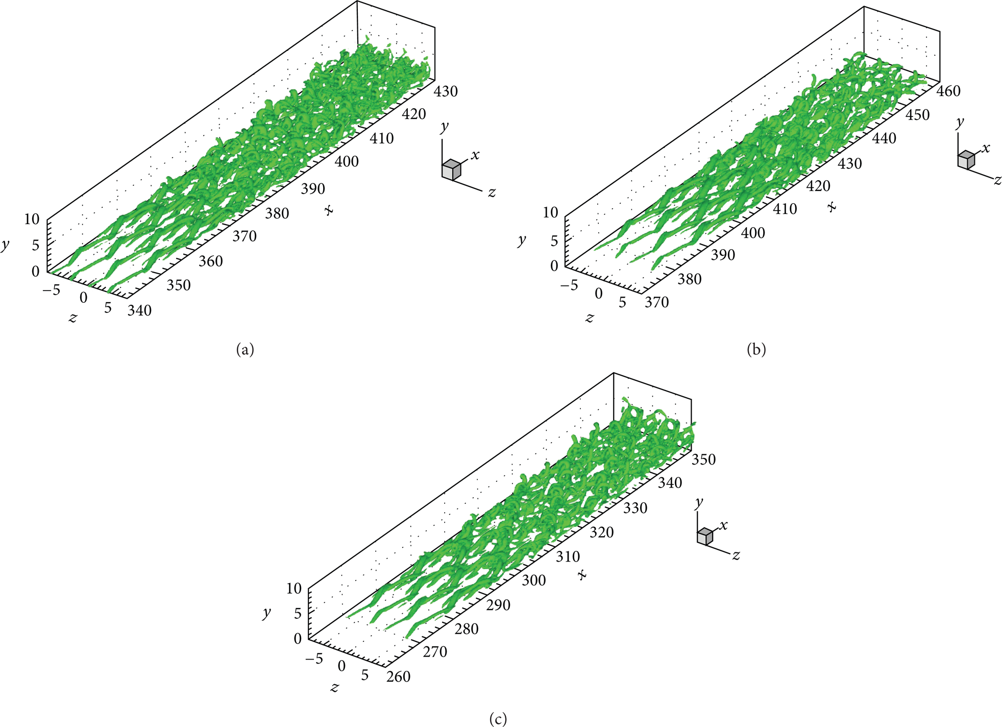
Instantaneous isosurface of Q = 0.02 with wall suction. (a) S2. (b) S3. (c) S5.

4. Conclusions and Remarks

In this paper, numerical research of boundary layer transition control is conducted through the spatial large eddy simulation method. The effects of wall cooling and suction on the supersonic boundary layer transition and turbulence over a flat-plate have been carried out. Some conclusions and remarks can be stated as follows.

The wall cooling is capable of delaying the onset of the spatially developing supersonic boundary layer transition. The transition control becomes more effective as the wall temperature drops, but the transition process will not completely stop under the cooling conditions given in the present simulations.

The wall suction can also be beneficial for delaying the transition process, but the effectiveness will be weakened once the wall suction reaches a certain intensity. In addition, the skin friction coefficient in the suction region increases significantly. Hence, one must take the impact of all factors into consideration when the suction is employed for controlling the transition.

The wall cooling and suction change the distributions of the mean velocity in the boundary layer, thereby improving the stability of the flow field. The boundary layer thickness decreases obviously with decreasing wall temperature and increasing wall suction intensity. The distributions of the turbulent Mach number increase significantly with decreasing wall temperature, indicating that the wall cooling can enhance the compressibility effects.

The development of large-scale coherent structures can be suppressed effectively via wall cooling. With decreasing wall temperature, the existence of Λ vortices, hairpin-like vortices, and ring-like vortices in the transition process gradually becomes not obvious. However, the wall suction has no influence on the development of large-scale coherent structures in transition process.

Conflict of Interests

The authors declare that there is no conflict of interests regarding the publication of this paper.

References

Adams

N. A.

and Kleiser

, “Subharmonic transition to turbulence in a flat-plate boundary layer at Mach number 4.5,” Journal of Fluid Mechanics, vol. 317, pp. 301–335, 1996.

Maeder

Adams

N. A.

, and Kleiser

, “Direct simulation of turbulent supersonic boundary layers by an extended temporal approach,” Journal of Fluid Mechanics, vol. 429, pp. 187–216, 2001.

Pirozzoli

Grasso

, and Gatski

T. B.

, “Direct numerical simulation and analysis of a spatially evolving supersonic turbulent boundary layer at M = 2.25,” Physics of Fluids, vol. 16, no. 3, pp. 530–545, 2004.

Sagaut

, Large Eddy Simulation for Incompressible Flows: An Introduction, Springer, New York, NY, USA, 3rd edition, 2006.

Piomelli

Zang

T. A.

Speziale

C. G.

, and Hussaini

M. Y.

, “On the large-eddy simulation of transitional wall-bounded flows,” Physics of Fluids A, vol. 2, no. 2, pp. 257–265, 1990.

Ducros

Comte

, and Lesieur

, “Large-eddy simulation of transition to turbulence in a boundary layer developing spatially over a flat plate,” Journal of Fluid Mechanics, vol. 326, pp. 1–36, 1996.

Normand

and Lesieur

, “Direct and large-eddy simulations of transition in the compressible boundary layer,” Theoretical and Computational Fluid Dynamics, vol. 3, no. 4, pp. 231–252, 1992.

Shan

Jiang

Zhao

, and Liu

, “Large eddy simulation of flow transition in a supersonic flat-plate boundary layer,” in Proceedings of the 37th Aerospace Sciences Meeting and Exhibit, AIAA paper 99-0425, Reno, Nev, USA, January 1999.

Stolz

Schlatter

, and Kleiser

, “Large-eddy simulations of subharmonic transition in a supersonic boundary layer,” AIAA Journal, vol. 45, no. 5, pp. 1019–1027, 2007.

10.

Reshotko

, “Control of boundary layer transition,” in Proceedings of the AIAA Shear Flow Control Conference, AIAA Paper 85-0562, Boulder, Colo, USA, March 1985.

11.

Kleiser

and Zang

T. A.

, “Numerical simulation of transition in wall-bounded shear flows,” Annual Review of Fluid Mechanics, vol. 23, no. 1, pp. 495–537, 1991.

12.

Kleiser

and Laurien

, “Numerical investigation of interactive transition control,” in Proceedings of the AIAA Shear Flow Control Conference, Boulder, Colo, USA, March 1985.

13.

Laurien

and Kleiser

, “Numerical simulation of boundary-layer transition and transition control,” Journal of Fluid Mechanics, vol. 199, pp. 403–440, 1989.

14.

Domaradzki

J. A.

and Metcalfe

R. W.

, “Stabilization of laminar boundary layers by compliant membranes,” Physics of Fluids, vol. 30, no. 3, pp. 695–705, 1987.

15.

Vreman

Geurts

, and Kuerten

, “Subgrid-modelling in LES of compressible flow,” Applied Scientific Research, vol. 54, no. 3, pp. 191–203, 1995.

16.

Wang

S. Z.

Gao

Z. X.

, and Lee

C. H.

, “Numerical investigation of compressibility effects in turbulent channel flows using large eddy simulation,” Science China Physics, Mechanics and Astronomy, vol. 55, no. 2, pp. 305–315, 2012.

17.

D. X.

and Ma

Y. W.

, “High order accurate schemes and numerical simulation of multi-scale structures in complex flow fields,” Acta Aerodynamica Sinica, vol. 16, no. 1, pp. 24–35, 1998 (Chinese).

18.

Lele

S. K.

, “Compact finite difference schemes with spectral-like resolution,” Journal of Computational Physics, vol. 103, no. 1, pp. 16–42, 1992.

19.

Gottlieb

and Shu

C.-W.

, “Total variation diminishing Runge-Kutta schemes,” Mathematics of Computation, vol. 67, no. 221, pp. 73–85, 1998.

20.

Dinavahi

S. P. G.

Pruett

C. D.

, and Zang

T. A.

, “Direct numerical simulation and data analysis of a Mach 4.5 transitional boundary-layer flow,” Physics of Fluids, vol. 6, no. 3, pp. 1323–1330, 1994.

21.

Kloker

Konzelmann

, and Fasel

, “Outflow boundary conditions for spatial Navier-Stokes simulations of transition boundary layers,” AIAA journal, vol. 31, no. 4, pp. 620–628, 1993.

22.

Wang

Gao

Lee

, and Lei

, “Large eddy simulation of supersonic boundary layer transition over a flat-plate based on the spatial mode,” Advances in Mechanical Engineering, vol. 2014, Article ID 350203, 10 pages, 2014.

23.

Dubief

and Delcayre

, “On coherent-vortex identification in turbulence,” Journal of Turbulence, vol. 1, no. 11, pp. 1–22, 2000.

Numerical Investigation of Wall Cooling and Suction Effects on Supersonic Flat-Plate Boundary Layer Transition Using Large Eddy Simulation

Abstract

1. Introduction

2. Numerical Simulation Method

3. Results and Discussion

3.1. Wall Cooling

3.2. Wall Suction

4. Conclusions and Remarks

Conflict of Interests

References