G EN D EP : Location-Aware Key Management for General Deployment of Wireless Sensor Networks

Abstract

Limited capabilities of tiny sensor node make it difficult to build a secure wireless sensor network. To cope with this problem, location-aware key predistribution schemes have been studied but without considering irregularity of real sensing fields. They were designed for ideal sensing fields divided into uniform regular polygons but false is the real sensing field, where we face irregular obstacles, undulations, and boundaries. In this paper, we tackle this problem from practical sense and first introduce the general deployment model, comparable to the previous uniform deployment model. To construct a secure WSN in the general deployment model, we present a new framework called GenDep, which consists of two phases: group placement and key management. In the group placement phase, we find an optimal position for sensor groups so that both connectivity and global coverage are satisfied for secure communications. In the key management phase, we devise a new structure called extended groups to partition the whole deployment area into irregular subareas. GenDep can build secure and flexible WSNs by using the existing key predistribution schemes even designed in the uniform deployment model. To ensure practicality of GenDep, we also conduct rigorous analysis and simulation in this paper.

1. Introduction

Wireless sensor networks (WSNs) play an important role in mission critical applications, such as military systems, healthcare services, and industrial systems. In such applications, security is a crucial requirement. Unfortunately, it is quite challenging to construct secure WSNs because tiny sensor nodes are very constrained in the capacity of computation, communications, storage, and power management. In particular, key management, which is the most fundamental part of security mechanisms, must be considered in the design phase of WSN with regard to the limited capabilities of tiny sensor nodes.

Since Eschenauer and Gligor have introduced the first proposal [1], a variety of approaches have been studied for secure key management based on the key predistribution concept [2–7]. Among them, location-aware key management schemes [5–7] were remarkable in their efficiency in terms of computation and communication costs (Section 2.1). Indeed, the efficiency came from the preknowledge of the location that helps sensor nodes share secret keys effectively with their (likely) adjacent nodes. However, previous approaches are unrealistic. (1) The previous deployment models assumed a sensing field to be a flat area that is dividable into uniform, regular grids. Such a uniform deployment model is, however, far from the real sensing field, which is actually not uniform in its geographical features and so highly inefficient. (2) The previous location-aware key management schemes are not applicable to a general deployment model, which covers various geographic features in the real sensing field. Their target application is so limited; nonuniform density was not allowed for placing the sensor nodes (Section 2.2).

To cope with these problems in this paper, we first present the general deployment model for WSNs and then propose a new location-aware key management framework called GenDep so as to be effective in that model. We can summarize our contribution as follows.

• (i)

We present the general deployment model (Section 3). We address that the conventional uniform models are unrealistic because geographical features are irregular in the real world. The general deployment model relaxes the constraints of sensing fields and implements the conceptual WSNs to be practical.

(ii)

On the general deployment model, we construct the new framework called GenDep that actually enables practical location-aware key management. GenDep consists of two phases. First, in the group placement phase (Section 4), we find optimal positions of sensor groups by fulfilling the requirements of WSN applications and geographical features. After placing groups of sensor nodes, we partition a whole sensing field into a number of nonuniform polygons, called zones. Second, in the key management phase (Section 5), we can employ the existing key predistribution schemes (even designed in the uniform deployment model) for our general deployment model. To do so, we devise a new structure of extended groups, each of which consists of a pair of adjacent zones. The extended groups are organized for every pair of zones; thus they overlap each other and connect all neighbors. We treat every extended group as an independent group. Therefore, we can employ any key predistribution scheme for each extended group.

(iii)

We evaluate GenDep via numerical analyses and simulations (Section 6). In particular, the numerical analyses handle connectivity, security, and storage overhead of sensor nodes with general probability distributions.

2. Background and Problem

2.1. Related Work

Sensor Node Placement. Previous studies on the node placement have focused on how to place a sensor node at an optimal location individually. Meguerdichian et al. addressed the coverage problem in WSN [8]. They calculated the maximum breach path and the maximum service path of nodes to find a position that maximizes coverage. In [9], Zou and Chakrabarty introduced a greedy algorithm called virtual force algorithm (VFA). VFA assumes targets have virtual attractive forces and obstacles have virtual repulsive forces. Sensor nodes can find their position under the influence of the forces. Zou and Chakrabarty [10] also proposed setting a virtual backbone from active nodes to improve coverage and connectivity in ad hoc networks. Takahara et al. [11] evaluated the coverage of sensors deployed in the grid pattern for uniform and normal errors. Wang et al. [12] proposed a deployment strategy when sensors are deployed in Gaussian distribution without concerns on the connectivity. Recently, interesting researches have been carried out to enhance coverage in mixed WSNs, which has the heterogeneous setting of static and mobile nodes. Ghosh and Das presented a good survey on the coverage and connectivity issues in [13]. Static sensor nodes are arranged to maximize the coverage (blanket/barrier coverage of [13]) and mobile sensor nodes move carefully to fill the coverage holes (sweep coverage). Lambrou and Panayiotou proposed collaborative scheme to improve coverage in mixed sensor networks [14, 15]. In particular, considering the tradeoff between coverage and energy consumption (communication), they pursue an autonomous sensor system to improve coverage effectively by mobile sensor nodes. Emphasizing the role of mobile sensor nodes for coverage, Das and Roy presented an algorithm to maximize coverage with continuous movement of sensor nodes in [16]. The proposed algorithm lets the mobile sensor nodes cover the sensing field fully within a fixed time. Mahboubi et al. employ Voronoi polygons in [17] to find the coverage holes. Each sensor node has its Voronoi polygon that is derived by relative position to adjacent nodes. Thus the difference between the sensing area and the Voronoi polygon can show the effectiveness of coverage. The authors proposed node-based and vertex-based strategies to relocate sensor nodes. He et al. presented curve-based deployment for barrier coverage in [18]. They modeled sensor nodes along curved lines to enhance the suboptimal coverage of line-based coverage. To sum up, the previous researches focused on placing individual sensor nodes effectively and achieved their goal. However, in large-scale WSNs, where sensors are deployed in groups, we have to take into account group placement. In that sense, GenDep focuses on placing sensor groups rather than individual sensor nodes.

Key Management in Wireless Sensor Networks. In [1], Eschenauer and Gligor proposed a random key predistribution (RKP) scheme for WSNs. A randomly selected sub-key pool is preinstalled to each node before deployment. Chan et al. enhanced RKP (q-composite RKP, qRKP).  qRKP achieves better resilience by restricting the minimum number of shared keys to connect. They also proposed the random-pairwise key scheme (RP) in [19], where RP selects a random pair and gives a pairwise key. In [3], Du et al. proposed a structured key-pool RKP scheme (skRKP) by adding randomness to the Blom scheme [20]. If two sensors share a key space, they can generate a key through shared key matrix. The location-aware schemes enhance key managements in WSN. They partition a whole sensing field into fixed square areas, called “grid.” We classify it as grid deployment. Du et al. proposed the location-aware RKP, where sensors share a key pool with other sensors in the same and adjacent grids only. Liu and Ning proposed a similar approach using bivariate polynomials [6]. In the grid-group key predistribution scheme (GGD) [5], Huang et al. employ skRKP to connect nodes in the same grid but RP to connect nodes in adjacent grids. Fanian et al. applied a mixed key from polynomial-based and random key predistribution schemes to WSNs in [21]. Grid-based predeployment knowledge on location is used to preinstall the hybrid keys to sensor nodes. Our previous work improves the connectivity in key management with perfect resilience via the key offering method [22].

2.2. Problems

Previous location-aware approaches [2, 3, 5, 6] assume the uniform deployment model, where a sensing field is a flat area with a uniform geographical feature. In real world, however, a target sensing field is nonuniform. We hardly meet the ideal sensing field that fits to the uniform deployment model. Furthermore, the real-world field has irregular geographical features. The WSN applications also have different sensing interests. Of course we can apply the uniform deployment model to the real-world field by force but it must be extremely inefficient.

Figure 1 shows an example of the real-world sensing field. Suppose that we would like to install WSN for a plain field only (not on the mountain and lake). We cannot make an optimal design to partition the sensing field with grids. To provide a practical WSN for real-world sensing fields, we should be able to divide the sensing field into any polygons like the dotted lines.

Figure 1

An example of the sensing field in the real world.

3. GenDep Overview

In this section, we overview the proposed method, GenDep, which is a novel location-aware key management scheme in the general deployment model. The detailed explanations on GenDep will be given in later sections, Sections 4 and 5.

3.1. General Deployment Model

Large-scale WSNs benefit from group-based deployment, that is, placing sensors by the unit of a group [23], for their scalability. Since sensor groups should be placed in a fixed pattern, however, the uniform deployment model is not appropriate for large-scale WSNs in the real world. To cope with this impracticality, we present the general deployment model. Any form of deployment area can be used for group-based deployment by dividing it into nonuniform subareas, which the existing uniform deployment model cannot support. The general deployment model relaxes the constraints and resolves this problem. Unfortunately, the previous location-aware key management schemes have been considered in the uniform model only, and so they are not quite workable in the general model. It is desirable to develop a new location-aware key management method in the general deployment model.

3.2. GenDep Framework

The new method proposed in this paper is called GenDep. In the general deployment model, GenDep divides and assigns subareas in irregular form to sensor groups and performs location-aware key management effectively.

Figure 2 illustrates the basic procedure of GenDep. Given the information of a sensing field and application requirements in the general deployment model, we firstly define the sensing requirements, which imply the required density of sensors at a particular point. We then apply GenDep in two phases as follows.

• (i)

Phase 1: in this phase, we make a group placement plan by finding optimal positions of “sensor groups.” We first set reference points according to the sensing requirements and then set deployment points of sensor groups based on the reference points. Finally, we adjust the planned location and distribution of sensor groups so as to enhance the intergroup connectivity.

(ii)

Phase 2: in this phase, we preinstall key sets and conduct location-based key establishment in the general deployment model. We first build group structures incorporating zones and extended groups. Second, we preinstall key sets to every sensor node so as to deploy sensor groups to the target sensing field according to the group placement plan. Finally, after the real deployment, all the sensor nodes conduct pairwise key establishment.

Figure 2

Procedure of GenDep.

4. Group Placement (Phase 1)

The group-based deployment phase consists of three steps: (1) setup reference points, (2) setup deployment points, and (3) adjust distributions. Notations section summarizes the notations to be used in this paper.

4.1. Step 1: Setup Reference Points

In this step, we set reference points according to the sensing requirements. First of all, we represent a target sensing field as a two-dimensional Cartesian plane and place reference points $(x,y)$ , as illustrated in Figure 3(a). The reference points are the points that hold sensing requirements at their position and are placed by following the uniform distribution. Note that they are not actual deployment points but only used for deriving local sensing requirements based on the prior knowledge about the terrain and WSN application.

Figure 3

Three steps of the group placement scheme. (All sensor groups are modeled as the Gaussian distribution with $\sigma =10.0$ .)

From [9, 10, 12, 24], we generalize the sensing requirements for the general deployment model. It is required that an event taking place at a certain reference point $(x,y)$ should be detected by at least $b(x,y)$ numbers of sensor nodes with the probability of $p_d(x,y)$ . Hence, the sensing requirements are defined at a specific point $(x,y)$ and parametrized as follows:

• (i)

$p_d(x,y)$ : detection probability of a sensor desired at $(x,y)$ ,

(ii)

$b(x,y)$ : number of sensors required to detect an event at $(x,y)$ .

We then combine these parameters to the sensor density desired at $(x,y)$ , $U(x,y)$ . First we compute the area of the sensing region where a sensor node can detect an event with higher probability than $p_d(x,y)$ . We assume probabilistic sensing model, in which the detection probability decays exponentially as the power of distance. When we suppose d is the distance of a sensor from an event, $e^{-\alpha d}$ would be the detection probability of the sensor, where α is a positive parameter that represents the physical characteristics of the sensor node and it is determined by the sensor type [9, 12]. Hence a sensor can detect an event taking place within $-(\ln p_d(x,y)/\alpha )$ with higher probability than $p_d(x,y)$ and the area of the sensing region is $\pi {\{-(\ln p_d(x,y)/\alpha )\}}^2$ when we assume sensors are omnidirectional. In other words, an event at $(x,y)$ can be detected by sensors located in the sensing region of $\pi {\{-(\ln p_d(x,y)/\alpha )\}}^2$ with the probability of $p_d(x,y)$ . $U(x,y)$ also requires at least $b(x,y)$ number of sensors to be located in the sensing region. Thus,

$$\begin{array}{cc}& U(x,y)=\frac{b(x,y)}{\pi {\left\{\ln p_d\left(x,y\right)/\alpha \right\}}^2}.\end{array}$$

(1)

However, $U(x,y)$ is a goal of density to achieve when deploying sensor nodes. When placing sensor nodes as a group, it is likely that there exists a gap between the goal $U(x,y)$ and the actual density of sensor nodes at $(x,y)$ . We represent the gap, $V(x,y)$ , as follows:

$$\begin{array}{l}V(x,y)\hfill \\ =\max \left(U(x,y)-{\displaystyle \sum }_{i=1}^{N_D}‍\frac{N_i\left(x,y,-(\ln p_d\left(x,y\right)/\alpha )\right)}{\pi {\left\{-(\ln p_d\left(x,y\right)/\alpha )\right\}}^2},0\right),\hfill \end{array}$$

(2)

where $N_D$ is the total number of sensor groups and $(N_i(x,y,-(\ln p_d(x,y)/\alpha )))/(\pi {\{-(\ln p_d(x,y)/\alpha )\}}^2)$ is the density of sensor nodes belonging to $i\text{th}$ sensor group, $G(i)$ at $(x,y)$ . Let us defer the explanation of $N_i(·)$ to Section 6.2.4.

Figure 3(a) shows an initial state of $V(x,y)$ when the target sensing field is covered by 25 reference points. With $\alpha =1$ , $U(x,y)$ is derived from the sensing requirements given to the reference point $(x,y)$ , that is, $p_d(x,y)$ and $b(x,y)$ . Since no sensor groups are deployed yet, $V(x,y)$ is the same as $U(x,y)$ for now.

4.2. Step 2: Setup Deployment Points

The goal of this step is to set deployment points of sensor groups on the positions that would minimize the sum of all $V(x,y)$ , that is, $\min {\sum }_{\forall (x,y)}‍V(x,y)$ . We first perform initial placement and then adjust the position of the deployment points.

Initial Placement. We conduct the initial deployment as shown in Algorithm 1. Algorithm 1 finds a reference point of highest $V(x,y)$ and assigns an unassigned sensor group at the point iteratively. Since $V(x,y)$ represents the gap between $U(x,y)$ and the sensor density of assigned sensor groups, the value of $V(x,y)$ keeps being updated during the process. As a result, we obtain the set B of assigned deployment points of sensor groups.

Algorithm 1: Initial placement: initial placement for unassigned sensor groups.

Input: A set $Q=\{G(i)\hspace{0.17em}|\hspace{0.17em}1\ge i\ge N_D\}$ of sensor groups and a set

    $W=\{\forall \left((x,y),V(x,y)\right)\}$ of tuples of a reference point $(x,y)$ and its

    $V(x,y)$ for every reference point

Output: A set $B=\left\{[x,y{]}_i\hspace{0.17em}|\hspace{0.17em}1\ge i\ge N_D\right\}$ of deployment points assigned to sensor groups

$B\leftarrow \mathrm{\varnothing }$

for   $G(i)\in Q$   do

  Find a reference point $(x,y)$ of highest $V(x,y)$ in W.

   $[x,y{]}_i\leftarrow (x,y)$ .

  Add $[x,y{]}_i$ to B.

  Update $V(x,y)$ s in W.

end

return  B

We will improve the result of initial placement in the following steps. We first adjust positions in B to minimize the sum of $V(x,y)$ . And then we determine an optimal position (in Step 3) with regard to the intergroup connectivity.

Position Adjustment. We present a new algorithm, pVFA, which adjusts the assigned deployment position of sensor groups to find more suitable position for achieving the goal. pVFA is an iterative, subgradient method. In an iteration of pVFA, every sensor group calculates a gradient that would decrease the sum of all $V(x,y)$ . The gradient is represented as an Euclidean vector (direction and magnitude) in the target sensing field. Sensor groups move along their gradients by a unit step at the end of an iteration.

More specifically, Algorithm 2 explains the detailed process. Let ${\overrightarrow{F}}_{G(i)}^A(x,y)$ be attractive force on a group $G(i)$ from a reference point $(x,y)$ . A reference point attracts sensor groups with the power of $V(x,y)$ ; that is, $\left|{\overrightarrow{F}}_{G(i)}^A(x,y)\right|=V(x,y)$ . The gradient of $G(i)$ , ${\nabla }_{G(i)}$ , is the sum of attractive power from all the reference points, ${\nabla }_{G(i)}={\sum }_{\forall (x,y)}‍{\overrightarrow{F}}_{G(i)}^A(x,y)$ . A sensor group, $G(i)$ , updates its assigned deployment point as $[{x+{\delta }_d·{\nabla }_{G(i)}|}_x,{y+{\delta }_d·{\nabla }_{G(i)}|}_y{]}_i$ by applying its gradient, where ${\delta }_d$ is a unit step for distance. The iteration is repeated until the average of gradients goes below a threshold $T_V$ .

Algorithm 2: Position adjustment: adjustment of initial position of sensor groups.

Input: A set $B=\left\{{\left[x,y\right]}_i\hspace{0.17em}|\hspace{0.17em}1\ge i\ge N_D\right\}$ of deployment points assigned to sensor groups

Output: A set $B^{\prime }=\left\{{\left[x,y\right]}_i\hspace{0.17em}|\hspace{0.17em}1\ge i\ge N_D\right\}$ of deployment points after position adjustment

repeat

   for   $G(i)\in Q$   do

    Calculate an attractive force, ${\overrightarrow{F}}_{G(i)}^A(x,y)$ , from $V(x,y)$ .

     $\left({{\overrightarrow{F}}_{G\left(i\right)}^A\left(x,y\right)|}_x=\left|V\left(x,y\right)\right|\cos \theta ,{\hspace{0.17em}{\overrightarrow{F}}_{G(i)}^A(x,y)|}_y=|V(x,y)|\sin \theta \right)$

    Derive the gradient of $G(i)$ : ${\nabla }_{G(i)}={{\displaystyle \sum }}_{\forall (x,y)}\mathrm{‍}{\overrightarrow{F}}_{G(i)}^A(x,y)$ .

    Update its position as ${\left[{x+{\delta }_d·{\nabla }_{G(i)}|}_x,{y+{\delta }_d·{\nabla }_{G(i)}|}_y\right]}_i$ of B

    Update $V(x,y)$ s in W.

   end

   Copy B to $B^{\prime }$ .

until   $T_V>\frac{{\sum }_{i=1}^{N_D}\mathrm{‍}\left|{\nabla }_{G(i)}\right|}{N_D}$

return   $B^{\prime }$

Figure 3(b) shows the results of this step. The circles indicate the effective region of sensor groups (which we will describe in the next step). The initial deployment determines the gray circles while the black circles indicate the position of sensor groups after the position adjustment. We show the gradient ${\nabla }_{G(i)}$ as a vector in arrow. As a result, we could obtain the intermediate deployment points of sensor groups and we will finalize the optimal deployment points in the next step.

4.3. Step 3: Adjust Distributions

The result of the previous step could have satisfied the sensing requirements (initially given by the general deployment model) but may have isolated groups having no well-connected adjacent groups because of missing the intergroup connectivity. To avoid such a case, we adjust the assigned deployment point and distribution of sensor groups before accomplishing the group placement plan.

The requirement for achieving “well-connectedness” in the intergroup connectivity is to have an effective, reasonable number of interconnections for two adjacent sensor groups. Thus, we count interconnections between sensor nodes, both of which are effective members in their own sensor groups only. To do so, we first define an effective region of a sensor group as the area covered by an effective number (we set the effective number as 80 percent of the number of sensor nodes in a group) of sensor nodes in that group. And we then set the minimum number of interconnections for two sensor groups to become a connected component.

Effective Region and Interconnections. We model sensor nodes deployed in a sensor group by omnidirectional probabilistic distributions, for example, Gaussian distribution. Hence the effective region is a circular region whose radius we calculate from the inverse cumulative distribution (CDF) [25] of the probabilistic distribution. CDF of the distribution of a sensor group returns the portion of member nodes for a given region of the sensor group; thus the inverse CDF provides an area (or a radius) that holds the given portion of sensor nodes. For example, we calculate the radius of the effective region as $P^{-1}(0.8)$ , where $P^{-1}()$ is the inverse CDF. We then regard interconnections of sensor nodes located in intersection of the effective regions of two adjacent sensor groups as effective interconnections. Let $w_i$ and $w_j$ , respectively, denote the number of sensor nodes from $G(i)$ and $G(j)$ in the intersection region between $G(i)$ and $G(j)$ .

Minimum Number of Interconnections. To become a connected component, a sensor group must have such a minimum degree of graph as $\lceil C\log n_z\rceil$ , where C is a tunable radio transmission range parameter ( $C\ge 1.5$ will increase the global connectedness to be close to 1) [26] and $n_z$ is the number of sensor nodes in a sensor group. Similarly, two sensor groups must have a minimum degree of graph, $\lceil C\log 2n_z\rceil$ . Therefore, we define a set of well-connected neighbor groups, ${\widehat{N}}_i$ , for group $G(i)$ :

$$\begin{array}{cc}& {\widehat{N}}_i=\left\{j\hspace{0.17em}|\hspace{0.17em}{p}_1^{*}·w_j\ge \lceil C\log 2n_z\rceil ,\hspace{0.17em}\forall j,i\ne j\right\},\end{array}$$

(3)

where $p_1^{*}$ is the probability that two nodes of different groups can be connected. It indicates that two nodes are within each other's communication range and also share keys because only sensor nodes sharing the same key can communicate with each other [5]. Finally, to avoid the case that isolated groups exist, the following condition should be satisfied:

$$\begin{array}{cc}& \left|{\widehat{N}}_i\right|\ge \lceil C\log N_D\rceil .\end{array}$$

(4)

pVFA with an Extending Option. We improve the intergroup connectivity of the isolated sensor groups by extending their effective regions. For this purpose, we employ pVFA with an extending option. Algorithm 3 shows the process of this step. First we compute the effective region, denoted by $F_i$ , of a group $G(i)$ and calculate intergroup connections between every pair of neighboring sensor groups, which have overlapped effective region in common. We then identify the isolated groups by using the condition of (4). When extending the effective region, we control the parameter of probability distribution of the sensor group. Here we suppose that we model the probability distribution as the two-dimensional Gaussian distribution. Thus we increase the standard deviation (std), ${\sigma }_i$ , of $G(i)$ by multiplying ${\delta }_s$ , which is a unit step for std. During extending the effective region, we can improve the connectivity but we could also experience the lower density of sensor nodes in the sensor group at the same time. It may bring back $V(x,y)$ . Thus pVFA also adjusts the position by applying the algorithm PositionAdjustment of Algorithm 2. This process is repeated until there is no isolated group and the average magnitude of the gradient is below $T_V$ . The result is a deployment plan for a given sensing field. The deployment plan indicates the position of sensor groups (i.e., deployment points) and its distribution parameter (i.e., std).

Algorithm 3: Final adjustment: adjustment of position and distribution for intergroup connectivity.

Input: A set $B^{\prime }=\left\{{\left[x,y\right]}_i\hspace{0.17em}|\hspace{0.17em}1\ge i\ge N_D\right\}$ of deployment points after position adjustment

Output: Deployment plan: a set $K=\left\{([x,y{]}_i,{\sigma }_i)\hspace{0.17em}|\hspace{0.17em}1\ge i\ge N_D\right\}$ of

     deployment points and distribution for each sensor group

$I\leftarrow \mathrm{\varnothing }$

repeat

   foreach   $G(i)$   do Compute the effective region of $G(i)$ , $F_i$

   for   $\forall (G(i),G(j))$ ,   $F_i\cup F_j\ne \mathrm{\varnothing }$   do

   Calculate inter-group connections between $G(i)$ and $G(j)$

   end

   Identify isolated groups as I

   for   $G(i)\in I$   do

    ${\sigma }_i\leftarrow {\delta }_s·{\sigma }_i$

   end

   Apply PositionAdjustment

until   $I\ne \mathrm{\varnothing }$   and   $T_V>\frac{{\sum }_{i=1}^{N_D}\mathrm{‍}\left|{\nabla }_{G(i)}\right|}{N_D}$

return  K

In Figure 3(c), the gray circle and the black circle indicate the effective region, respectively, before and after the adjustment. We could observe that isolated groups have extended their effective regions while several groups have moved to minimize $V(x,y)$ in Figure 3(c). Compared with the result of Step 2, the fraction of connected groups has been significantly improved from 0.455 to 1.0 at the cost of $V(x,y)$ , of which the average increased from 0.0043 to 0.0132.

5. Key Management (Phase 2)

In this section, we describe the key management phase of GenDep. On the basis of the result of the group placement phase, we preinstall key sets to sensors for establishing pairwise keys in the key management phase. To do so, we describe building group structures in Step 1, preinstalling key sets to sensors in Step 2, and establishing pairwise keys in Step 3 (after deployment).

5.1. Step 1: Build Group Structures

In order to provide the location awareness to the key management schemes, we need to define a zone for a group. The key management schemes assume zones are nonoverlapped; thus we divide the sensing field into zones by using the Voronoi decomposition method [27], where a Voronoi cell for a seed point is a region consisting of points that are closer to the seed point than other seed points.

By employing the deployment points of groups as the seed points, we define a zone for the group $G(i)$ is the Voronoi cell based on its deployment point, $[x,y{]}_i$ . Let $N{V}_i$ denote a set of groups sharing Voronoi edges with the group $G(i)$ . Then we could define a set of neighbor groups, $NZ(i)$ , as follows:

$$\begin{array}{cc}& NZ\left(i\right)=N{V}_i\cap {\widehat{N}}_i.\end{array}$$

(5)

Figure 4(a) is an example of the zones based on the deployment points of Figure 3. The sensing field was partitioned into 11 zones. Every zone has different shapes and different neighbors. In order to explain the subsequent process more clearly, we use the field of Figure 4(b) that consists of various polygons, that is, irregular zones.

Figure 4

Voronoi decomposition and deployment plan.

After partitioning zones, every pair of two neighboring zone groups is merged to be an extended group, EG. A group belongs to as many EGs as the number of its neighbor groups.

Algorithm 4 explains the process for setting the neighbor sensor group and assigning extended groups. All the assigned EGs are in E. In addition, Figure 5 illustrates an example of multiple EGs (i.e., 5 EGs) overlapped on the group $G(7)$ . Note that EGs could intrinsically support location awareness because of binding a pair of adjacent zones.

Algorithm 4: Build structure: define the neighbor groups and build a set of extended groups of every pair of neighboring sensor groups.

Input: A set Q of sensor groups, a set $N_i$ of well-connected sensor groups of

    $G(i)$ , and a set $N{V}_i$ of the sensor groups sharing a Voronoi edge with $G(i)$

Output: A set $E=\{\mathsf{E}\mathsf{G}(i,j)\hspace{0.17em}|\hspace{0.17em}G(j)\in NZ(i)\vee G(i)\in NZ(j)\}$ of extended groups.

$E\leftarrow \mathrm{\varnothing }$

foreach   $G(i)$   do

   $NZ(i)\leftarrow N{V}_i\cap {\widehat{N}}_i$

  for   $G(j)\in NZ(i)$   do

   if  EG $(i,j)\notin W$   then

        $E\leftarrow E\cup \{\mathsf{E}\mathsf{G}(i·j)\}$

   end

  end

end

return  E

Figure 5

Group structures for group $G(7)$ . (Note that $\mathsf{E}\mathsf{G}(i,j)$ denotes the extended group of $G(i)$ and $G(j)$ .)

5.2. Step 2: Preinstall Key Sets

In this step, we assign key predistribution schemes to EGs and preinstall key sets to be used for key establishment. Before preinstall keys to sensor nodes, we select a key predistribution scheme suitable for each EG. Because each EG is an independent space, we could assign not only homogeneous but also heterogeneous key predistribution schemes to EGs. It is clear that heterogeneous schemes could only affect their own EGs. For example, a compromised sensor node may only contaminate sensors in its local EG. When selecting key predistribution schemes, we could flexibly approach them by considering their distinct features in terms of node-capture resilience, storage overhead, and computational complexity. We could prioritize one of those features in each EG. For instance, we could select RP for prioritizing the perfect resilience against node capture attacks or RKP for higher connectivity. No key predistribution scheme is a panacea.

According to the selected key predistribution schemes, we preinstall key sets to sensor nodes. Algorithm 5 shows the procedure. First we assign unique identifiers, $\text{I}{\text{D}}_u$ and $\text{I}{\text{D}}_{\mathsf{E}\mathsf{G}}$ , to each sensor node and each EG, respectively. For each EG, we generate a key pool, ${\mathcal{K}}_{\mathsf{E}\mathsf{G}(i,j)}$ , according to the selected key predistribution scheme for the EG. From the key pool, we select a key set and install it on a sensor node of the EG. The method for generating a key pool GenerateKeyPool and selecting a key set from the key pool SelectKeysFrom is dependent on the selected key predistribution scheme.

Algorithm 5: Preinstall: preinstall a key set for each sensor node.

Input: A set E of extended groups

foreach a sensor node, u  do

  SetNewIdentifier   $\left(u,I{D}_u\right)$

end

foreach  EG $(i,j)$   do

  SetNewIdentifier   $(\mathsf{E}\mathsf{G}(i,j),I{D}_{\mathsf{E}\mathsf{G}})$

   ${\mathcal{K}}_{\mathsf{E}\mathsf{G}(i,j)}$ ←  GenerateKeyPool $(\mathsf{E}\mathsf{G}(i,j))$

  for a sensor node, $u\in \mathsf{E}\mathsf{G}(i,j)$   do

   s←  SelectKeysFrom $({\mathcal{K}}_{\mathsf{E}\mathsf{G}(i,j)})$

   InstallKeySet $(u,s)$

  end

end

5.3. Step 3: Establish Pairwise Keys

Finally, we could deploy sensor nodes into the sensing field. After deployment, the sensor nodes will then establish pairwise keys by themselves. The procedure to establish pairwise keys is as follows.

• (1)

Key Discovery. Each sensor node broadcasts its ID, $\text{I}{\text{D}}_u$ , and key list whereas the key list is composed of the identifiers of its keys, $〈\text{I}{\text{D}}_k,\text{I}{\text{D}}_{\mathsf{E}\mathsf{G}}〉$ . Sensor nodes could exchange them with their neighbors and compare the lists for key establishment.

(2)

Pairwise Key Establishment. If a sensor node finds a neighbor node sharing the same key, then it sends a connection request to the neighbor. By using the key agreement method of [3], the two adjacent nodes can generate a pairwise key in a secure way.

(3)

Path Key Establishment. If there remain neighbors not yet connected, the sensor node broadcasts the IDs of the disconnected neighbors to the connected neighbors, so that the connected neighbors could help them to establish pairwise keys. This step is repeated until the sensor node connects to all the neighbors and cannot find newly connectable nodes.

6. Performance Evaluation

In this section, we analyze the performance of GenDep. We compare our method to the previous location-aware key management schemes based on the fixed deployment model, such as GGD [5] and skRKP [2].

6.1. System Model for Evaluation

We assume the following.

• (i)

The number of sensor nodes ( $n_z$ ) is 100 in a single group.

(ii)

To compare the result with the previous schemes fair, we set each zone to be formed as a square: $\forall G(i),L_{G(i)}=4$ .

(iii)

GenDep uses three configurations for key predistribution schemes: G-skRKP, G-COMB, and G-RP. For G-skRKP and G-RP, we select skRKP and RP as key predistribution schemes, respectively. In G-COMB, a combination of RKP and RP is applied; among 4 EGs of a group, 2 EGs use RKP and the other 2 EGs employ  RP. The key pool size of the RKP scheme is 4880 to keep the faction of communication compromised under 0.4 until 50% nodes are compromised [1].

(iv)

In order to keep the same level of key storage and to preserve the λ-secure property (for resilience against compromised sensor nodes, the key distribution schemes using the secret key matrix of the Blom scheme, such as GGD and skRKP [2, 5], have an upper bound on the ratio of the number of sensor nodes and the size of secret matrix; this is called λ-secure property; please refer to [3] for the λ-secure property) [3], $\omega =7$ for all the schemes but ${\tau }_G=3$ , ${\tau }_D=2$ , and ${\tau }_E=1$ for GGD, skRKP-D, and G-skRKP, respectively. The analysis of key storage is described in Section 6.5. Additionally, we set the parameters for GGD as ${\gamma }_{\mathtt{G}\mathtt{G}\mathtt{D}}=8$ and ${\alpha }_{\mathtt{G}\mathtt{G}\mathtt{D}}=1$ based on [5].

6.2. Key Graph Connectivity

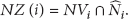
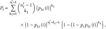
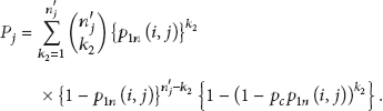
Let $p_{1n}(i,j)$ be the probability that two sensor nodes in $G(i)$ and $G(j)$ share at least one common key. It is assumed that a sensor node of $\mathsf{E}\mathsf{G}(i,j)$ randomly picks $m_k$ different keys for $\mathsf{E}\mathsf{G}(i,j)$ from a key pool of size M. Then, the $p_{1n}(i,j)$ is

$$\begin{array}{l}{p}_{1n}\left(i,j\right)=1-\frac{\left(\begin{array}{l}M\hfill \\ m_k\hfill \end{array}\right)\left(\begin{array}{l}M-m_k\hfill \\ m_k\hfill \end{array}\right)}{{\left(\begin{array}{l}M\hfill \\ m_k\hfill \end{array}\right)}^2}\hfill \\ =1-\frac{{\left\{\left(M-m_k\right)!\right\}}^2}{M!·\left(M-2m_k\right)}.\hfill \end{array}$$

(6)

Likewise, let $p_{1s}(i)$ be the probability that two sensor nodes in the same $G(i)$ share at least one common key. The sensor nodes in the same group have all their EGs in common. They can be connected unless they do not share any key in their EGs, which are $\mathsf{E}\mathsf{G}(i,j),G(j)\in NZ(i)$ . For each $\mathsf{E}\mathsf{G}(i,j)$ that they share, the key graph connecting probability is $p_{1n}(i,j)$ . Thus,

$$\begin{array}{cc}& p_{1s}\left(i\right)=1-{\displaystyle \prod }_{G\left(j\right)}^{NZ\left(i\right)}‍\left(1-p_{1n}\left(i,j\right)\right).\end{array}$$

(7)

If a single key predistribution scheme is applied to all EGs of $G(i)$ , $p_{1s}(i)$ is calculated as

$$\begin{array}{l}{p}_{1s}\left(i\right)=1-{\left[\frac{\left(\begin{array}{l}M\hfill \\ m_k\hfill \end{array}\right)\left(\begin{array}{l}M-m_k\hfill \\ m_k\hfill \end{array}\right)}{{\left(\begin{array}{l}M\hfill \\ m_k\hfill \end{array}\right)}^2}\right]}^{L_{G\left(i\right)}}\hfill \\ =1-{\left[\frac{{\left\{\left(M-m_k\right)!\right\}}^2}{M!\left(M-2m_k\right)!}\right]}^{L_{G\left(i\right)}},\hfill \end{array}$$

(8)

since the number of shared EGs of the two sensor nodes in the same group is $L_{G(i)}$ . Appendix A shows the probabilities, $p_{1n}$ and $p_{1s}$ , on the instantiations of key predistribution schemes in GenDep.

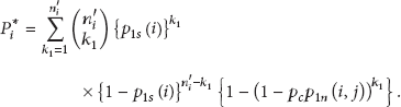
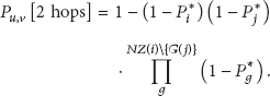
A sensor node can be connected to neighbors directly (1 hop) or through relaying of other neighbor nodes (more than 1 hop). For simplicity and clarity, we consider 2 hops at maximum. Let $N_i(x,y,R)$ be the number of sensors of $G(i)$ within the communication range R from a position $(x,y)$ . We assume a sensor node u in $G(i)$ at $(x,y)$ . For the sensor node u, we take $n_i^{\prime }=N_i(x,y,R)-1$ as the number of reachable neighbor nodes in $G(i)$ (the number of sensor nodes within the communication range except itself) and $n_j^{\prime }=N_j(x,y,R)$ as the number of reachable neighbor nodes in $G(j)$ , where $j\ne i$ and $G(j)\in NZ(i)$ .

6.2.1. Key Graph Connectivity within the Same Group

Suppose that a sensor node u connects to another sensor node v in the same group $G(i)$ , $u,v\in G(i)$ . We represent the probability that two nodes are connected, $P_{u,v}$ , as

$$\begin{array}{cc}& P_{u,v}=P_{u,v}\left[1\mathrm{\hspace{0.17em}\hspace{0.17em}}\text{hop}\right]+\left(1-P_{u,v}\left[1\mathrm{\hspace{0.17em}\hspace{0.17em}}\text{hop}\right]\right)P_{u,v}\left[2\mathrm{\hspace{0.17em}\hspace{0.17em}}\text{hops}\right],\end{array}$$

(9)

where the probability of the 1-hop connection, $P_{u,v}[1\mathrm{\hspace{0.17em}\hspace{0.17em}}\text{hop}]$ , is equal to $p_{1s}(i)$ . When we calculate the probability of the 2-hop connection, $P_{u,v}[2\mathrm{\hspace{0.17em}\hspace{0.17em}}\text{hops}]$ , we take account of two cases of relaying: by a node in the same group or another node in a neighbor group. Let us denote by $P_i$ and $P_j$ the probabilities that the sensor nodes, u and v, are connected via a node in $G(i)$ and $G(j)\in NZ(i)$ , respectively. The two nodes can be connected in any of these cases. Hence,

$$\begin{array}{cc}& P_{u,v}\left[2\mathrm{\hspace{0.17em}\hspace{0.17em}}\text{hops}\right]=1-\left(1-P_i\right)·{\displaystyle \prod }_{G\left(j\right)}^{NZ\left(i\right)}‍\left(1-P_j\right).\end{array}$$

(10)

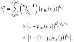
We calculate $P_i$ and $P_j$ by developing the binomial probability distribution (the development of the binomial probability distribution for the key graph connecting probability is inspired by [28]). We compute $P_i$ as follows:

$$\begin{array}{l}{P}_i={\displaystyle \sum }_{k_1=1}^{n_i^{\prime }-1}\left(\begin{array}{l}\hfill n_i^{\prime }-1\hfill \\ \hfill k_1\hfill \end{array}\right){\left\{p_{1s}\left(i\right)\right\}}^{k_1}\hfill \\ \hspace{1em}\hspace{1em}\times {\left\{1-p_{1s}\left(i\right)\right\}}^{n_i^{\prime }-k_1-1}\left\{1-{\left(1-p_c{p}_{1s}\left(i\right)\right)}^{k_1}\right\},\hfill \end{array}$$

(11)

where the part ${\sum }_{k_1=1}^{n_i^{\prime }-1}‍\left(\begin{array}{c}{n}_i^{\prime }-1\\ k_1\end{array}\right)\{p_{1s}(i){\}}^{k_1}\{1-p_{1s}(i){\}}^{n_i^{\prime }-k_1-1}$ is the binomial probability distribution that represents that u is connected to $k_1$ sensor nodes out of $n_i^{\prime }-1$ neighbors (the number of reachable neighbor nodes except v) and u is connected to one of $k_1$ sensor nodes by $p_{1s}(i)$ . The term, $1-(1-p_c{p}_{1s}(i){)}^{k_1}$ , represents the probability that at least one of the $k_1$ sensor nodes is connected to v. Note that $p_c$ is the probability that any two sensor nodes are within the communication range of each other. If the communication range is circle-shaped and of equal radius, then $p_c$ is 0.5865 regardless of R according to [28]. Likewise, we calculate $P_j$ as

$$\begin{array}{l}{P}_j={\displaystyle \sum }_{k_2=1}^{n_j^{\prime }}‍\left(\begin{array}{l}{n}_j^{\prime }\\ k_2\end{array}\right){\left\{p_{1n}\left(i,j\right)\right\}}^{k_2}\hfill \\ \times {\left\{1-p_{1n}\left(i,j\right)\right\}}^{n_j^{\prime }-k_2}\left\{1-{\left(1-p_c{p}_{1n}\left(i,j\right)\right)}^{k_2}\right\}.\hfill \end{array}$$

(12)

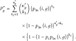
Equation (12) represents that u is connected to v via one of $k_2$ sensor nodes in $G(j)\in NZ(i)$ . Since the $k_2$ sensor nodes belong to $G(j)$ , the connecting probability between them and u or v is $p_{1n}(i,j)$ . Finally, we get (13) by joining (9), (10), (11), and (12).

$$\begin{array}{l}{P}_{u,v}\\ =p_{1s}\left(i\right)+\left(1-p_{1s}\left(i\right)\right)\\ \hspace{1em}\times \{1-[1-{\displaystyle \sum }_{k_1=1}^{n_i^{\prime }-1}‍\left(\begin{array}{l}{n}_i^{\prime }-1\\ k_1\end{array}\right){\left\{p_{1s}\left(i\right)\right\}}^{k_1}\\ \hspace{1em}\hspace{1em}\hspace{1em}\hspace{1em}\hspace{1em}\hspace{1em}\hspace{1em}\hspace{1em}\times {\left\{1-p_{1s}\left(i\right)\right\}}^{n_i^{\prime }-k_1-1}\\ \hspace{1em}\hspace{1em}\hspace{1em}\hspace{1em}\hspace{1em}\hspace{1em}\hspace{1em}\hspace{1em}\times \left\{1-{\left(1-p_c{p}_{1s}\left(i\right)\right)}^{k_1}\right\}\phantom{\left(\begin{array}{l}{n}_i^{\prime }-1\\ k_1\end{array}\right)}]\\ \hspace{1em}\hspace{1em}\hspace{1em}·{\displaystyle \prod }_j^{NZ\left(i\right)}‍[1-{\displaystyle \sum }_{k_2=1}^{n_j^{\prime }}‍\left(\begin{array}{l}{n}_j^{\prime }\\ k_2\end{array}\right){\left\{p_{1n}\left(i,j\right)\right\}}^{k_2}\\ \hspace{1em}\hspace{1em}\hspace{1em}\hspace{1em}\hspace{1em}\hspace{1em}\hspace{1em}\hspace{1em}\hspace{1em}\times {\left\{1-p_{1n}\left(i,j\right)\right\}}^{n_j^{\prime }-k_2}\\ \hspace{1em}\hspace{1em}\hspace{1em}\hspace{1em}\hspace{1em}\hspace{1em}\hspace{1em}\hspace{1em}\hspace{1em}\times \left\{1-{\left(1-p_c{p}_{1n}\left(i,j\right)\right)}^{k_2}\right\}\phantom{\left(\begin{array}{l}{n}_j^{\prime }\\ k_2\end{array}\right)}]\}\end{array}$$

(13)

6.2.2. Key Graph Connectivity between Neighbor Groups

$P_{u,v^{*}}$ is the probability that a sensor node u in $G(i)$ connects to another node v in $G(j)$ , that is, a neighbor group of $G(i)$ ( $G(j)\in NZ(i)$ ) with or without help from all neighbor nodes. Obviously, $P_{u,v^{*}}[1\mathrm{\hspace{0.17em}\hspace{0.17em}}\text{hop}]=p_{1n}(i,j)$ , but, in $P_{u,v^{*}}[2\mathrm{\hspace{0.17em}\hspace{0.17em}}\text{hops}]$ , three cases of 2-hop connections are possible: $P_i^{*}$ , $P_j^{*}$ , and $P_g^{*}$ .

First, $P_i^{*}$ , the probability of 2-hop connection by relaying of a sensor node in $G(i)$ is

$$\begin{array}{l}{P}_i^{*}={\displaystyle \sum }_{k_1=1}^{n_i^{\prime }}‍\left(\begin{array}{l}\hfill n_i^{\prime }\hfill \\ \hfill k_1\hfill \end{array}\right){\left\{p_{1s}\left(i\right)\right\}}^{k_1}\hfill \\ \hspace{1em}\hspace{1em}\times {\left\{1-p_{1s}\left(i\right)\right\}}^{n_i^{\prime }-k_1}\left\{1-{\left(1-p_c{p}_{1n}\left(i,j\right)\right)}^{k_1}\right\}.\mathrm{\hspace{0.17em}\hspace{0.17em}}\hfill \end{array}$$

(14)

In (14), note that $p_{1s}(i)$ and $p_{1n}(i,j)$ , respectively, represent the probability that node u connects to $k_1$ neighbor nodes and the probability that $k_1$ neighbor nodes connect to node v. Second, $P_j^{*}$ is the probability of 2-hop connection by relaying of a sensor node in $G(j)$ and is given as

$$\begin{array}{l}{P}_j^{*}={\displaystyle \sum }_{k_2=1}^{n_j^{\prime }-1}‍\left(\begin{array}{l}\hfill n_j^{\prime }-1\hfill \\ \hfill k_1\hfill \end{array}\right){\left\{p_{1n}\left(i,j\right)\right\}}^{k_2}\hfill \\ \hspace{1em}\hspace{1em}\times {\left\{1-p_{1n}\left(i,j\right)\right\}}^{n_j^{\prime }-k_2-1}\hfill \\ \hspace{1em}\hspace{1em}\times \left\{1-{\left(1-p_c{p}_{1s}\left(j\right)\right)}^{k_2}\right\}.\hfill \end{array}$$

(15)

Third, $P_g^{*}$ is the probability of 2-hop connection by the relay of a sensor node in neighbor groups except $G(j)$ , which are $NZ(i)\setminus \{G(j)\}$ . Hence, $P_g^{*}$ is

$$\begin{array}{l}{P}_g^{*}={\displaystyle \sum }_{k_3=1}^{n_g^{\prime }}‍\left(\begin{array}{l}\hfill n_g^{\prime }\hfill \\ \hfill k_3\hfill \end{array}\right){\left\{p_{1n}\left(i,g\right)\right\}}^{k_3}\hfill \\ \hspace{1em}\hspace{1em}\times {\left\{1-p_{1n}\left(i,g\right)\right\}}^{n_g^{\prime }-k_3}\hfill \\ \hspace{1em}\hspace{1em}\times \left\{1-{\left(1-p_c{p}_{1n}\left(i,g\right)\right)}^{k_3}\right\}.\hfill \end{array}$$

(16)

From (14), (15), and (16), we derive that

$$\begin{array}{l}{P}_{u,v}\left[2\mathrm{\hspace{0.17em}\hspace{0.17em}}\text{hops}\right]=1-\left(1-P_i^{*}\right)\left(1-P_j^{*}\right)\hfill \\ ·{\displaystyle \prod }_g^{NZ\left(i\right)\setminus \left\{G\left(j\right)\right\}}‍\left(1-P_g^{*}\right).\hfill \end{array}$$

(17)

Finally,

$$\begin{array}{cc}& P_{u,v^{*}}=P_{u,v^{*}}\left[1\mathrm{\hspace{0.17em}\hspace{0.17em}}\text{hop}\right]+\left(1-P_{u,v^{*}}\left[1\mathrm{\hspace{0.17em}\hspace{0.17em}}\text{hop}\right]\right)P_{u,v^{*}}\left[2\mathrm{\hspace{0.17em}\hspace{0.17em}}\text{hops}\right].\end{array}$$

(18)

Joining (14), (15), (16), and (17), we represent $P_{u,v^{*}}$ as (19).

$$\begin{array}{l}{P}_{u,v^{*}}\\ =p_{1n}(i,j)+(1-p_{1n}(i,j))\\ \hspace{1em}·\{1-[1-{\displaystyle \sum }_{k_1=1}^{n_i^{\prime }}‍\left(\begin{array}{l}{n}_i^{\prime }\\ k_1\end{array}\right){\left\{p_{1s}\left(i\right)\right\}}^{k_1}\\ \hspace{1em}\hspace{1em}\hspace{1em}\hspace{1em}\hspace{1em}\hspace{1em}\hspace{1em}\hspace{1em}\times {\left\{1-p_{1s}\left(i\right)\right\}}^{n_i^{\prime }-k_1}\\ \hspace{1em}\hspace{1em}\hspace{1em}\hspace{1em}\hspace{1em}\hspace{1em}\hspace{1em}\hspace{1em}\times \left\{1-{\left(1-p_c{p}_{1n}\left(i,j\right)\right)}^{k_1}\right\}\phantom{\left(\begin{array}{l}{n}_i^{\prime }\\ k_1\end{array}\right)}]\\ \hspace{1em}\hspace{1em}\hspace{0.5em}·[1-{\displaystyle \sum }_{k_2=1}^{n_j^{\prime }-1}‍\left(\begin{array}{l}{n}_j^{\prime }-1\\ k_1\end{array}\right){\left\{p_{1n}\left(i,j\right)\right\}}^{k_2}\\ \hspace{1em}\hspace{1em}\hspace{1em}\hspace{1em}\hspace{1em}\hspace{1em}\hspace{1em}\hspace{1em}\times {\left\{1-p_{1n}\left(i,j\right)\right\}}^{n_j^{\prime }-k_2-1}\\ \hspace{1em}\hspace{1em}\hspace{1em}\hspace{1em}\hspace{1em}\hspace{1em}\hspace{1em}\hspace{1em}\times \left\{1-{\left(1-p_c{p}_{1s}\left(j\right)\right)}^{k_2}\right\}\phantom{{\displaystyle \sum }_{k_2=1}^{n_j^{\prime }-1}‍}]\\ \hspace{1em}\hspace{1em}\hspace{0.5em}·{\displaystyle \prod }_g^{NZ\left(i\right)\setminus \left\{G\right(j\left)\right\}}‍[1-{\displaystyle \sum }_{k_3=1}^{n_g^{\prime }}‍\left(\begin{array}{l}{n}_g^{\prime }\\ k_3\end{array}\right)\left(\begin{array}{l}\\ \end{array}\right){\left\{p_{1n}\left(i,g\right)\right\}}^{k_3}\\ \hspace{1em}\hspace{1em}\hspace{1em}\hspace{1em}\hspace{1em}\hspace{1em}\hspace{1em}\hspace{1em}\hspace{1em}\hspace{1em}\hspace{0.5em}\hspace{1em}\times {\left\{1-p_{1n}\left(i,g\right)\right\}}^{n_g^{\prime }-k_3}\\ \hspace{1em}\hspace{1em}\hspace{1em}\hspace{1em}\hspace{1em}\hspace{1em}\hspace{1em}\hspace{1em}\hspace{1em}\hspace{1em}\hspace{0.5em}\hspace{1em}\times \left\{1-{\left(1-p_c{p}_{1n}\left(i,g\right)\right)}^{k_3}\right\}\phantom{{\displaystyle \sum }_{k_3=1}^{n_g^{\prime }}‍}]\phantom{{\displaystyle \sum }_{k_3=1}^{n_g^{\prime }}‍}\}\end{array}$$

(19)

6.2.3. Numerical Results in Key Graph Connectivity

Figure 6 depicts $P_{u,v}$ and $P_{u,v^{*}}$ when $n_i^{\prime }$ and $n_j^{\prime }$ are the same. Table 1 shows the parameters, $p_{1s}$ and $p_{1n}$ , computed by the equations as referred to Appendix A. As illustrated in Figure 6, the connectivity of GGD is best at the same group but worst between the neighbor groups at the same time. The reason is that GGD employs different methods for the same and the neighbor groups. The connectivities at the same group are similar in G-skRKP, G-RP, and skRKP-D. But the connectivities between the neighbor groups are better than skRKP-D in G-skRKP and G-RP as illustrated in Figure 6(b). When we assume the number of neighbor nodes is 21, in Figure 6(a), the $P_{u,v}$ of G-RP is $22\%$ and $3\%$ lower than GGD and skRKP-D, respectively, but, in Figure 6(b), $P_{u,v^{*}}$ of G-RP is $640.7\%$ and $55.7\%$ higher than the two schemes. In other words, GenDep has slightly lower connectivity within the same group but far higher connectivity between the neighbor groups. In both cases of Figure 6, G-COMB achieves high connectivity. Furthermore, it is noteworthy that RP is a good choice as a key predistribution scheme because G-RP shows better performance than skRKP-D and G-skRKP. In addition, RP does not require complex computation in the key establishment and has better network resilience [22].

Table 1

Local connectivity ( $p_{1s}$ and $p_{1n}$ ).

	$p_{1s}$	$p_{1n}$
G GD	0.8857	0.01
skRKP-D	0.5338	0.0816
G-skRKP	0.4602	0.1429
G-RP	0.4779	0.15
G-COMB	0.62	0.33 (RKP), 0.08 (RP)

Figure 6

Key graph connectivity.

6.2.4. Discussion on Key Graph Connectivity according to Deployment Distribution

We model the deployment method for a sensor group as probabilistic distribution of sensor nodes. In this section, we take into consideration two kinds of probabilistic distributions: Gaussian and uniform distributions.

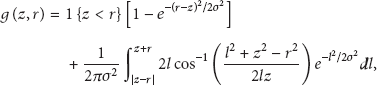
Gaussian Distribution. First, in the Gaussian distribution, sensor nodes are deployed in the 2-dimension (2D) Gaussian distribution from their deployment point. We denote by $g(z,r)$ the cumulative density function (CDF) of the 2D Gaussian distribution within a circle whose center is located at the distance of z from the deployment point and its radius is r. More formally,

$$\begin{array}{l}g\left(z,r\right)=1\left\{z<r\right\}\left[1-e^{-{\left(r-z\right)}^2/2{\sigma }^2}\right]\hfill \\ +\frac{1}{2\pi {\sigma }^2}{{\displaystyle \int }}_{\left|z-r\right|}^{z+r}‍2l\hspace{0.17em}{\cos }^{-1}\left(\frac{l^2+z^2-r^2}{2lz}\right)e^{-l^2/2{\sigma }^2}dl,\hfill \end{array}$$

(20)

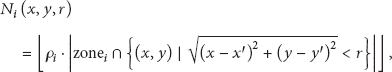
where σ is the standard deviation of the Gaussian distribution. Please refer to [29] about derivation of $g(z,r)$ . Let us denote the position of the deployment point, $[x,y{]}_i$ , by using $x_i$ and $y_i$ . The number of nodes in $G(i)$ at the point of $(x,y)$ within r is

$$\begin{array}{cc}& N_i\left(x,y,r\right)=\lfloor n_z·g(\sqrt{{\left(x-x_i\right)}^2+{\left(y-y_i\right)}^2},r)\rfloor .\end{array}$$

(21)

Figure 7 depicts the probability of the key graph connectivity to nodes in any neighbor group, $P_{*}=1-{\prod }_k^{NZ}‍(1-P_{u,v^{*}})$ , from (0,0) to (100,100) where the deployment point is located at (50,50). Since the distribution of neighbor nodes determines the probability of the key graph connectivity, Figure 7 shows high connectivity along each direction to the deployment points of neighbor groups. Additionally, note that the shape of the zone in Figure 7(a) is a regular polygon, that is, a square, but that of Figure 7(b) is the irregular pentagon, which is the same shape to the zone G in Figure 4(b).

Figure 7

Key graph connectivity with Gaussian sensor deployment ( $n_z=100$ , $\sigma =25$ , $r=10$ , $\mathtt{G}\text{-}\mathtt{s}\mathtt{k}\mathtt{R}\mathtt{K}\mathtt{P}$ ).

Uniform Distribution. Second, in the uniform distribution, the coverage area and density determine the number of neighbor nodes regardless of the deployment point. Let ${\rho }_i$ be the sensor node density of $G(i)$ , which can be calculated by ${\rho }_i=n_z/\left|\text{zon}{\text{e}}_i\right|$ , where $\text{zon}{\text{e}}_i$ is the zone of $G(i)$ . Hence, the number of sensor nodes within r in $G(i)$ is

$$\begin{array}{l}{N}_i(x,y,r)\hfill \\ \hspace{1em}=\lfloor {\rho }_i·\left|\text{zon}{\text{e}}_i\cap \left\{\left(x,y\right)\hspace{0.17em}|\hspace{0.17em}\sqrt{{\left(x-x^{\prime }\right)}^2+{\left(y-y^{\prime }\right)}^2}<r\right\}\right|\rfloor ,\hfill \end{array}$$

(22)

where $\left|\text{zon}{\text{e}}_i\cap \{(x,y)\hspace{0.17em}|\hspace{0.17em}\sqrt{(x-x^{\prime }{)}^2+(y-y^{\prime }{)}^2}<r\}\right|$ is the area of the intersected region between $\text{zon}{\text{e}}_i$ and the communication range of the node located at $(x^{\prime },y^{\prime })$ . The intersected area can be calculated geometrically using the sensor coverage analysis such as [5].

6.3. Simulation

We perform simulation to validate our analysis result in more realistic situations. Our simulation follows the system setup of Sections 6.1 and 6.2.4 ( $n_z=100$ , $\sigma =25$ , $R=10\hspace{0.17em}\text{m}$ ). In the simulation, we place nine sensor groups as shown in Figure 8. Each group is located from a given group distance. We ran simulation with varying distances between groups to check the number of connections to confirm the trends of key graph connectivity of our analysis in Section 6.2.3. In the simulation, we implemented GGD and G-skRKP, since the relative performance of G-skRKP to GGD is a good indicator for the trend of the analysis result.

Figure 8

Simulation setting. We place nine sensor groups and deploy sensor nodes in Gaussian distribution. (Please note that we use $\sigma =10$ in this figure to show sensor groups more distinguishably but $\sigma =25$ in the simulation to follow the settings of Sections 6.1 and 6.2.4.)

Figure 9 shows the result of the simulation. We change the distance between groups from 20 m to 50 m and count the total number of connections established within the two-hop key graph after deployment. Since sensor nodes are deployed randomly in Gaussian distribution, we ran simulation 30 times to get the average of the results. As expected, we can observe that the connectivity within the same group does not change by varying the distance in Figure 9(a). GGD has 18.8% more connections among sensor node within the same group than G-skRKP. As shown in Figure 9(b), however, G-skRKP always outperforms GGD by 338% in the number of connections among neighbor groups. Therefore, both results show the same trend as the result of the numerical analysis in Section 6.2.3 and G-skRKP can provide higher connectivity between groups.

Figure 9

Key graph connectivity in the simulation.

6.4. Security Analysis

The group structures in GenDep prevent the general deployment model from incurring additional security concerns. The security conditions for the key predistribution schemes, such as the λ-secure property, can also be applied easily.

Figure 10 depicts the network resilience against node capture attacks for the same size of key sets, $m_k=30$ , and the local connectivity, $p_1=0.14$ . We refer to [3, 19] and Appendix B for the equations of the network resilience. In Figure 10, skRKP shows the strong resistance to the node capture attacks when $n_z$ is only restricted under 100, that is, satisfying the λ-secure property. However, RP can achieve the perfect resilience against the node capture attacks. Note that the network resilience of qRKP is worse than RKP due to the small size of $m_k$ and key pool. Therefore, we exclude the qRKP scheme in the performance comparison. In case that nodes store a relatively smaller number of keys for an EG, the RKP scheme is better to be selected for security and connectivity than the qRKP scheme.

Figure 10

Network resilience of the key predistribution schemes ( $m_k=30$ , $p_1=0.14$ ).

6.5. Storage Overhead

The size of the key storage required to preinstall key sets in a sensor node is dependent on the key predistribution schemes. Let $m_{k,l}$ be the size of the key storage for the $l\text{th}$ EGof a sensor node. The total storage for a node can be computed as $m={\sum }_{l=1}^{L_{G(i)}}‍m_{k,l}$ . The security conditions of the key predistribution scheme may restrict the lower bound of   $m_k$ . In that sense, for the Blom-based schemes in GenDep, the security parameter λ is calculated as $2n_z{\tau }_E/\omega$ . That is, the selected key space in GenDep, ${\tau }_E$ , should be half of τ that other Blom-based schemes use in order to keep the same value of $n_z$ . Thus, $m_k$ for an EG with skRKP   is

$$\begin{array}{cc}& m_k=\left(\lceil \frac{2n_z{\tau }_E}{\omega }\rceil +1\right){\tau }_E.\end{array}$$

(23)

In case that skRKP is assigned to all EGs, for example, G-skRKP, $m=L_{G(i)}·m_k$ . Table 2 shows the key storage overhead on various configurations for this case. Based on the configurations of [3, 5] ( $\omega =7$ , $\tau =2$ , ${\tau }_E=1$ , 64-bit key), the required key storage for GenDep is under a few kilobytes for both cases of $L_{G(i)}=4$ (rectangular zone) and $L_{G(i)}=6$ (hexagonal zone). Even in the cases of hexagonal zone, 128-bit key, and ${\tau }_E=2$ , the key storage is under 12 kbytes. Since MICAz sensor nodes have a 128 kbyte program memory and a 512 kbyte secondary memory [30], the required key storage is small enough to be installed to the memory of sensor nodes.

Table 2

Required key storage.

L	$n_z$	ω	${\tau }_E$	Key size (bits)	Storage (bytes)	L	$n_z$	ω	${\tau }_E$	Key size	Storage
4	50	7	1	64	512	6	50	7	1	64	768
4	100	7	1	64	960	6	100	7	1	64	1440
4	200	7	1	64	1888	6	200	7	1	64	2832
4	50	7	1	128	1024	6	50	7	1	128	1536
4	100	7	1	128	1920	6	100	7	1	128	2880
4	200	7	1	128	3776	6	200	7	1	128	5664
4	50	7	2	64	1920	6	50	7	2	64	2880
4	100	7	2	64	3776	6	100	7	2	64	5664
4	200	7	2	64	7424	6	200	7	2	64	11136

Let $m_G$ , $m_D$ , $m_{\mathtt{G}\text{-}\mathtt{s}\mathtt{k}\mathtt{R}\mathtt{K}\mathtt{P}}$ , $m_{\mathtt{G}\text{-}\mathtt{C}\mathtt{O}\mathtt{M}\mathtt{P}}$ , and $m_{\mathtt{G}\text{-}\mathtt{R}\mathtt{P}}$ be the required storages to store keys for GGD, skRKP-D, G-skRKP, G-COMB, and G-RP, respectively. In skRKP-D, each key pool is shared among neighbor zones in proportion to a or b. In other words, due to the λ-secure property, we cannot deploy more than $n+(4a+4b)n$ nodes. Hence, $\lambda =\lceil n{\tau }_G/\omega \rceil$ for GGD and $\lambda =\lceil 2n{\tau }_D/\omega \rceil$ for skRKP-D using the condition $4a+4b=1$ in [2]. From these conditions, the required key storage for the schemes is

$$\begin{array}{cc}& m_G=\left(\lceil \frac{n_z{\tau }_G}{\omega }\rceil +1\right){\tau }_G+\gamma \alpha ,\\ m_D=\left(\lceil \frac{2n_z{\tau }_D}{\omega }\rceil +1\right){\tau }_D,\\ m_{\mathtt{G}\text{-}\mathtt{s}\mathtt{k}\mathtt{R}\mathtt{K}\mathtt{P}}=4\left(\lceil \frac{2n_z{\tau }_E}{\omega }\rceil +1\right){\tau }_E.\end{array}$$

(24)

From (24), the parameters of the system model in Section 6.1 are determined to achieve the same level of key storage, $m_D=m_{\mathtt{G}\text{-}\mathtt{s}\mathtt{k}\mathtt{R}\mathtt{K}\mathtt{P}}=120$ and $m_G=128$ . Since G-RP and G-COMB do not require the security conditions on m, we set the $m_{\mathtt{G}\text{-}\mathtt{C}\mathtt{O}\mathtt{M}\mathtt{P}}=m_{\mathtt{G}\text{-}\mathtt{R}\mathtt{P}}=120$ .

7. Conclusion

In this paper, we proposed GenDep, the novel framework for location-aware key management in WSNs regarding the general deployment model. Due to the notion of generalized location awareness, GenDep can apparently provide a practical advantage. The WSN can be deployed without losing its security in the real world where nonuniform geographical features exist. In GenDep, the group placement phase is operated to find optimal deployment positions of sensor groups. In the following key management phase, a whole deployment area is partitioned into a number of different smaller zones based on the deployment points of sensor groups. Subsequently, we build a new group structure to cover all sensor nodes deployed in neighboring zones. Using the group structures, we can render the benefit of location awareness to the existing key predistribution schemes. We proved the superior performance of key predistribution schemes when applied to GenDep, compared to their raw deployment. We also showed that it is possible to achieve the same level of security even in the irregular deployment area due to our generalized location awareness.

The generalized location awareness approach is promising for various practical applications, not limited to WSNs. For WSNs, GenDep enables their deployment to unforeseen circumstances. Thus GenDep is also applicable to three-dimensional (3D) sensor deployment, such as sensors in intelligent buildings. Secure key management for a group of any scattered devices can adopt GenDep as well, for example, RF readers in department stores and remote consoles in cafes and restaurants. We believe it would be promising to scrutinize more applications in the future study.