
Abstract
A self-propelled swimming fish model is established, which can reflect the interaction between fish movement, internal force generated by muscle contraction, and the external force provided by fluid. Using finite element immersed boundary method combined with traditional feedback force method, the self-propelled swimming fish is numerically simulated. Firstly, a self-induced vibration of a cantilever beam immersed in a fluid is one of the benchmarks of fluid-structure interaction, which is used to verify the validity of the numerical method. Secondly, start and cruise process of a single swimming fish in a straight-line swimming state is simulated and analysis of the flow characteristics and fish body movement features is done. The results reveal that the fish gain energy from flow field by the conversion of “C” type and “S” type of fish body.
1. Introduction
Study on the interaction between fluid and floating or flying creatures is usually applied to the bionics and reveals the mechanism of interaction between biological motion and fluid. Investigation of hydrodynamic characteristics of fish swimming can be traced to the invention of ancient boat and oars. In ancient times, people saying “a scull three pulp,” “namely, the scull efficiency is about three times the oar,” shows the efficiency of fish swinging. So, the modeling and simulation of fish-like swimming are of interest in life sciences as well as in engineering applications. More generally, many other technological applications ranging from the sedimentation of granular flows to the simulation of a maneuvering aircraft can benefit from the efficient modeling of the unsteady interaction between the flow and moving objects.
Among the first mathematical results concerning fish-like swimming were those reported by Lighthill [1, 2]. Since then, many other papers were dedicated to the study of inviscid flows of fish swimming [3]. A more recent fish-like swimming example is presented in [4–7]. But the traditional numerical method for biological fluid-structure interaction (FSI) problems has some limitations in large deformation of biological tissue, complicated structure, and calculation efficiency. How to establish an ideal numerical approach to deal with biological tissue in fluid-structure interaction problems has become the focus of researchers.
Motivated by these facts, in this paper we study fish-like swimming in the two-dimensional low Reynolds number case. Even though the experimental results cited are relevant to three-dimensional flows at a Reynolds number such that the flow is in the turbulent regime [8–11], the two-dimensional laminar case is of interest since numerical results for viscous flows and considering the energy provided by muscle in a fish-like swimming model are scarce. Also, the self-propelled fish swimming includes several fields of coupling, such as the fish body kinematics, the fluid dynamics, and structure dynamics as well as the internal force fields provided by muscle contraction, which is a complex FSI problem. Some researchers define the swimming form of the fish [12], but the freedom of swimming is limited. Others [13, 14] use an inverse approach; namely, they start with the measured kinematics and then estimate the hydrodynamic forces on the body and then the muscle forces required to generate the prescribed kinematics. Animal movements result from a complex balance of many different forces. Muscles produce force to move the body; the body has inertial, elastic, and damping properties that may aid or oppose the muscle force; and the environment produces reaction forces back on the body. So, study on hydrodynamic characteristics of fish swimming needs to establish an ideal fish swimming physical model, and the influence of key factors on hydrodynamic characteristics of fish swimming includes fish body shape, internal structure of fish, the energy produced by muscles, and external fluid. This is the main innovation in this paper due to the fact that the force produced by muscles is considered.
Handling well large deformation structure and/or moving boundaries is a major challenge in simulations of real natural flows, which requires creative approaches for mesh generation and boundary condition implementation. Many methods, including dynamical grid [15, 16], immersed boundary methods [17, 18], level set methods [19, 20], and penalization methods [21, 22] have been developed and successfully applied to specifically address this challenge. In particular, major advances in immersed boundary methods, such as the concept of grid generation and the idea of modeling the presence of a solid body by appropriate volume forces, as well as discretizing with a single, fixed, nonboundary conforming mesh system, which are of interest in this work, have made it possible to efficiently study flow problems that are far more complicated than those that traditional computational fluid dynamics methods could handle in the past [23–26].
In this paper, the fish-like swimming as the research object, using finite element immersed boundary method combined with the feedback force method [27–30], a flexible 2D model of freely self-propelled swimming fish that interacts between internal forces, fish body movement, and fluid, is established, and the fish is divided into three sections, namely, head, tail, and tail fin. This model of fish presented here includes an actuated, elastic body, based on that of a 2D fish swimming in a fluid domain. The motion of the body emerges as a balance between internal muscular force and external fluid forces. The hydrodynamic performance of a single swimming fish and fish schooling is numerically simulated.
2. Continuous Formulation of Immersed Boundary Method
In the IB formulation, the fluid is described by the Navier-Stokes equations in the Eulerian form and the structure is described by a viscous hyperelastic model in the Lagrangian form. A physical region Ω contains a fluid and an immersed structure. When the structure moves in the fluid region, let β identify the reference region of the elastic structure and let ∂β denote the boundary of ∇

Lagrange and Euler coordinate systems.
In the immersed boundary method formulation, an external force is added to the N-S equation, and this reflects the influence of solid on fluid. The density of fluid is ρ f and the elastic structure is ρ s . Assume for simplicity that ρ f = ρ s = ρ, so the Navier-Stokes (N-S) equations in Ω are

where

Equations (1)–(2) are the control equations of immersed boundary method and the key of this method is the information transfer between Lagrange variables and Euler variables. The traditional method is to use the Dirac delta approximation functions as δ(

In this paper, the four-Cartesian-point two-dimensional form of δ(
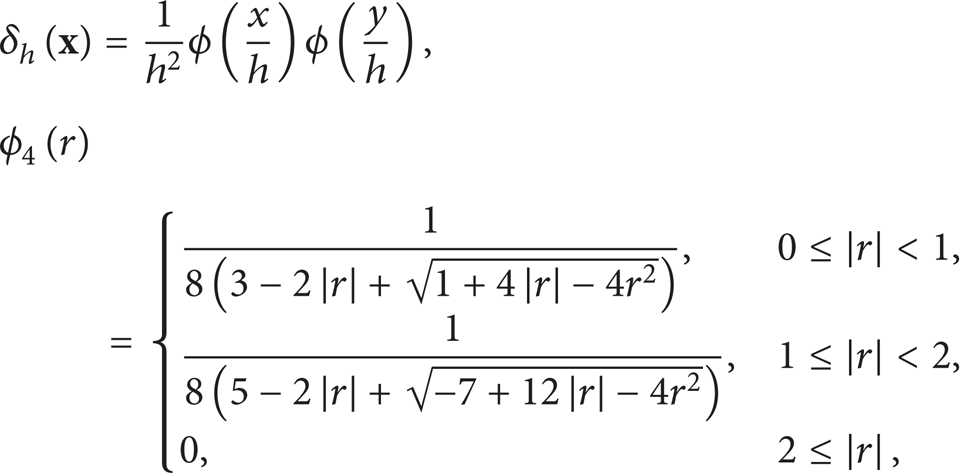
where h = Δx = Δy is grid scale. Through δ(
In (5),
2.1. Solving F
To solve the solid force density, it is needed to establish solid constitutive laws. According to different materials of the structure, two kinds of mechanical models (hyperelastic constitutive model and rigid model) are used in this paper.
2.1.1. Elastic Constitutive Model
The elastic structure is solved by finite element method in Lagrangian coordinate system, and it is convenient to express the stress in the reference (Lagrange) variables. Here, we use the first Piola-Kirchhoff elastic stress tensor field
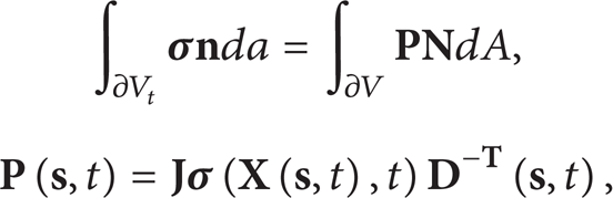
where
For any virtual displacement or Lagrangian test function
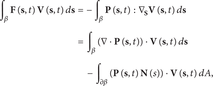
where
The constitutive law of the elastic structure is defined by hyperelastic models, and the typical model is the St. Venant-Kirchhoff elasticity model (STVK) and neo-Hookean model (INH).
The strain-energy functional W
s
(
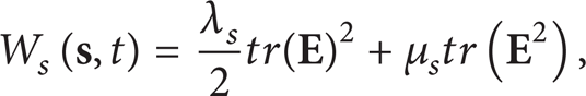
where
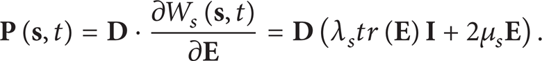
The strain-energy functional Ws(

The first P-K stress tensor in this case becomes

On the other hand, the entire physical system including fluid and elastic structure was enforced incompressibility because of the principle of IBM. Elastic material parameters
2.1.2. Rigid Model
For the rigid structure, this paper uses the feedback force immersed boundary method, and the equation can be written as

where κ
s
(
3. Discretization of the Immersed Boundary Formulation
3.1. Finite Difference Discretization of N-S Equations
Using a Cartesian staggered grid, the N-S equation is discretized by finite difference method in space. We assume that Ω is a 1 × 1 square region and is discretized on a regular N × N grid with grid spacing Δx = Δy = h = 1/N, as shown in Figure 2. The pressure p is approximated at the black points of the grid cells, such as (i – 1,j), (i,j), and (i + 1,j), and the components of Eulerian velocity field
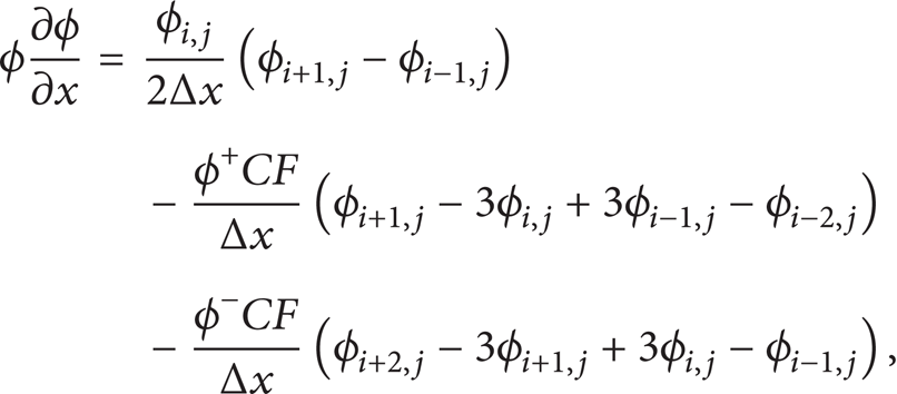
where
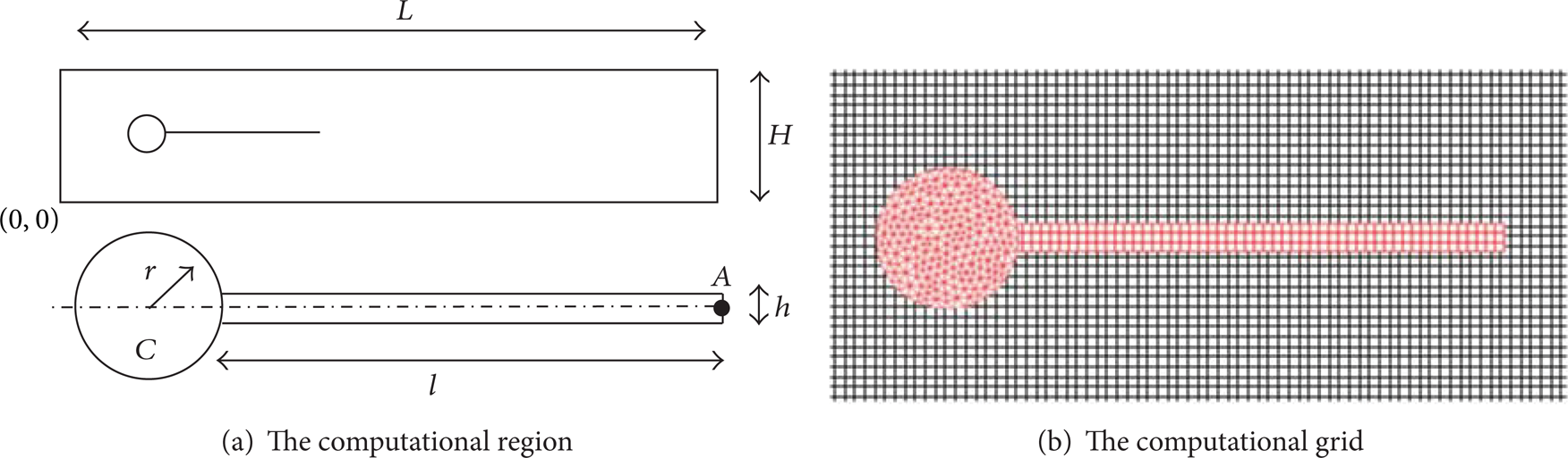
Computational region and grid for FSI-C numerical example.
3.2. Finite Element Discretization of Structure
The finite elements are generated for the structure β. β is composed of elements β
h
e
, and

while, in the nodes of the mesh,

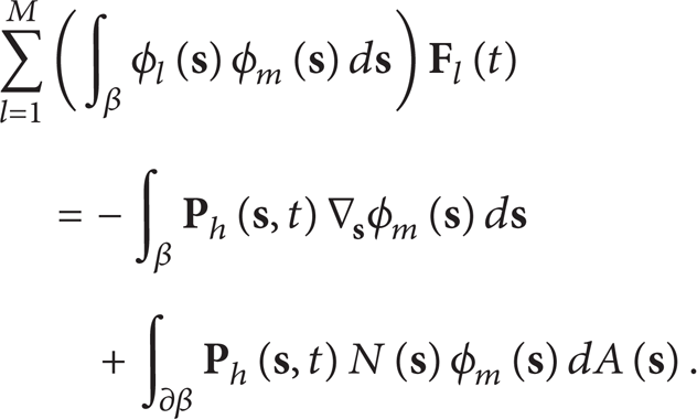
Using the constitutive laws of the structure, the
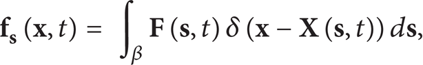
The Lagrangian force density
3.3. Discretion of Fluid-Structure Interaction Equations
The equations of fluid and structure interaction are (5) and (6). The fluid-structure interactions (5) and (6) are approximated by a smoothed function δ
h
(

The shorthand form can be written as
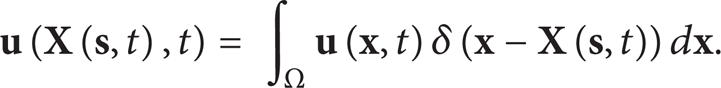
The Eulerian velocity field

The shorthand form can be written as
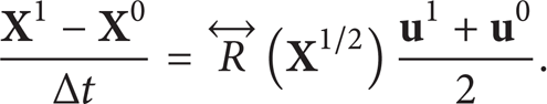
3.4. Time Discretization
Let Δt denote the time step, and, at time n·Δt = t
n
, we approximate the values of
Given the approximation
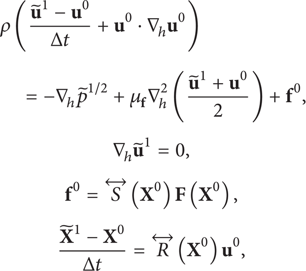
First, we preliminary compute

Then we define an approximation to
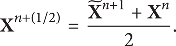
Using

We find the solutions

We correct

Because time step-lagged values of
Given the values of
where we let
We compute

We correct


When the values of
4. The Verification Example of IBM
4.1. The Establishment of Computational Model
Figure 2(a) is the computational domain of channel flow. A static rigid cylinder is immersed in fluid, a cantilever beam is attached to the cylinder. The self-induced oscillation of a cantilever beam immersed in a fluid (FSI-C) is one of the benchmarks of fluid-structure interaction. The elastic beam has width h = 0.02 m and length l = 17.5h. The computational domain has length L = 125h and width H = 20h. The center of cylinder is C = (10h, 10h), as the coordinate origin is set in left bottom corner, and the radius of cylinder is r = 2.5h. A control point A fixed at the trailing edge of the structure is with initial position (30h, 10h). The quadrilateral finite element mesh of the beam and uniform Cartesian grid of the fluid are used, as shown in Figure 2(b).
The upper and lower boundary and solid surface is no-slip wall boundary condition.
A parabolic velocity profile is prescribed at the left channel inflow:

where
The starting procedure for the nonsteady tests was to use a smooth increase of the velocity profile against time, namely,

Zero normal traction and zero tangential slip boundary conditions are used along the outflow. The no-slip condition is prescribed for the fluid on the top and bottom wall as well as cylinder surface.
For this benchmark problem, the fluid is assumed as incompressible and Newtonian. The fluid properties are ρ
f
= 1.0 × 10³ kg/m3 and ν
f
= 1.0 × 10⁻³ m2/s. The mass density of the elastic beam is the same as the fluid, and a STVK model is used to describe the elasticity of the beam with μs = 2.0 × 10⁶ kg/(ms2) and Poisson ratio νs = 0.4. The mean inflow velocity is
4.2. Analysis of Computational Results
We set κs = 1.0 × 10¹¹, and the total time of calculation is 20's. This benchmark is usually used to verify the reliability of numerical algorithm of fluid-structure interaction. The results of the benchmark are summarized in Table 1, and other reference values of Table 1 are derived from paper [31, 32]. Comparisons will be done particularly for one full period of the oscillation of the beam with respect to the position of the point A at the end of the beam structure (see Figure 2). In Table 1, v x (A) and v y (A) are the displacement in x- and y-direction of the point A in a period of vibration of beam, and the frequencies fx and fy are obtained for the displacements v x (A) and v y (A), respectively. The drag and lift forces F D and F L can be written as

where S denotes the structure being in contact with the fluid and
Comparison of the computational results between other papers and this paper.

Time dependent values are represented by mean value (me), amplitude (am), and frequency. The mean value and the amplitude are computed from the last period of the oscillations by taking the maximum(max) and minimum(min) values; namely, me = (max + min)/2 and am = (max-min)/2. In Table 1, the computational results of this paper are all within the range of results obtained by other numerical methods, which verify the reliability of this method in this paper.
5. The Establishment of Self-Propelled Swimming Fish Model
In this paper, in order to simulate the interaction between internal forces, fish body movement, and fluid, a volume force is added and acted on the tail of the fish and the force is simplified from internal forces produced by muscle, which is reflected truly by the real physiological condition of fish swimming. The coordinate of point A is (0.2, 0), which is used to output the fish displacement and velocity results of fish-like movement. The fish is considered as isotropic INH hyperelastic material and using the NACA0012 airfoil represents the body of fish, as shown in Figure 3. The total length is 1 m, and the fish body is divided into three sections, namely, head (0–0.5 m), tail (0.5–0.96 m), and tail fin (0.96–1 m). The coordinate of point A is (0.2, 0), which is used to output the fish displacement and velocity results.
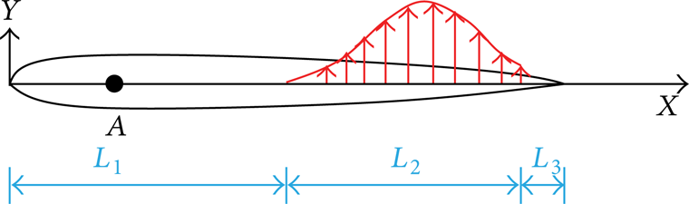
Model of fish.
Fish-like swim only along the -X direction is considered in this paper; then the control of the self-propelled swimming fish model is as follows.
(1) Head Section (L1). An elastic constraint is added in Y direction using feedback force method and this control formulation is

where κ
s
(
(2) Tail Section (L2). The internal force produced by muscle is simplified by adding a volumetric force on the tail section of fish body. At first, this volumetric force is loaded in + Y direction, and the tail begins to move. When an arbitrary point of the tail swings to a specified location, the direction of the volumetric force reverses, and the tail begins to swing to -Y direction. And then the direction of the volume force changes again when an arbitrary point of the tail swings to a specified location on the other side. Direction of the volumetric force is repeated to reverse, which simulated the periodic swing of the tail. The distribution of the volumetric force density on the tail section is

where
(3) Caudal Fin Section (L3). This section of the body is not controlled, and the elastic modulus is E3.
6. Numerical Simulation of Single Fish Swimming
6.1. The Establishment of Computational Model
The computational domain has length L = 20 m and width H = 3 m, as shown in Figure 4. A control point P fixed at the head of the fish with initial position (1.6 m, 1.5 m) as the coordinate of left bottom corner is (0, 0). The elastic coefficient in Y-direction on head section is κ
s
(

Computational region for the single swimming fish.
The fluid is static at the initial time, and the fluid density and kinematic viscosity are ρ f = 1.0 × 10³ kg/m3 and ν f = 1.0 × 10⁻⁶ m2/s, respectively. The mass density of the fish is the same as the fluid, and the elastic modulus of head and caudal fin section is E1 = E3 = 2.4 × 10⁶ Kg/(ms2) and the tail section is E2 = 2.4 × 10⁶ Kg/(ms2). The maximum volumetric force density is Fy_max = 1.5 × 10⁶ N/(m3).
In the whole computational domain of fluid using four layers adaptive Cartesian grid, the minimum grid spacing is 0.0045 m. The triangular finite element mesh for the fish is used, and the mesh number is 2090, as shown in Figure 5.
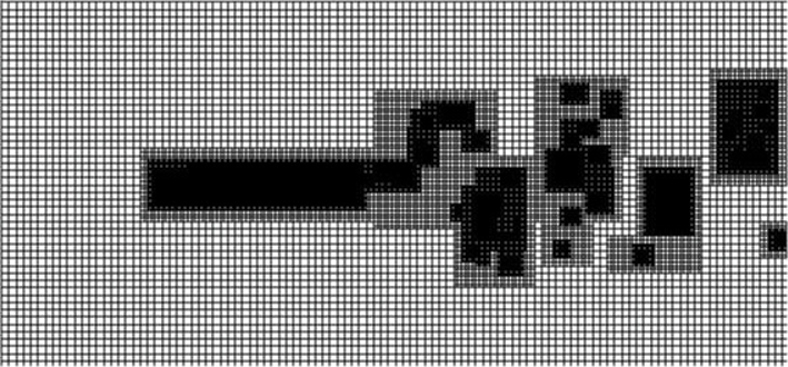
The grid for the swimming fish.
6.2. Analysis of Computational Results
Figure 6 shows fluid motion around the fish during steady swimming. A strong vortex sheds along the tail of caudal fin each time and forms the anti-Kármán vortex street when the tail swings back to the symmetry axis of fish body. Multiple weak secondary vortices are also produced from the head of the fish and move along body and shed finally at the tail of caudal fin.
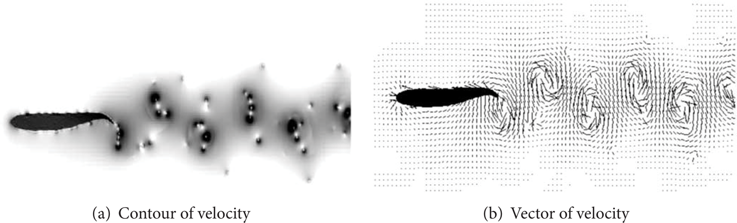
The anti-Kármán vortex street to the swimming fish.
Figure 7 shows the swimming speed from t = 0 s to a steady-state speed; in a whole, the form of swimming speed is similar to the results of paper [33]. It is seen that the velocity is gradually increased from t = 0 s to 3.0's, and then the swimming speed is up to a stable status. Also, we can see that the speed is fluctuant and increases, which is mainly affected by the periodical swing of the tail; simultaneously, there is small fluctuation in a period, which is attributed to the shedding of the weak secondary vortices along the fish body.

The swimming speed against time.
Figure 8 shows the flow distribution and fish shape during start-up process of swimming. The fish body has become “S” shape affected by the fluid dynamic force when the tail is moving opposed to the axis of body, and the body has become “C” shape when tail is moving back to the axis of body. The numerical simulation result of fish-like swimming is similar to the result of experiment [34]. There is a negative acceleration in 0–0.07's, as shown in Figure 7(b). After 0.07s, the fish began to accelerate motion until 0.22's. It can be seen that the tail moves up away to the axis of body from 0.07's, and the tail fin is passively sloping down and the fish body gradually becomes “S” shape until 0.14's. To “S” shape of upmovement, the pressure acted on the two sides of tail fin will contribute to accelerate the motion of fish, which is shown in Figure 9. Subsequently, the fish tail moves down back to the axis of body, and the tail fin is passively sloping up and the fish body gradually becomes “C” shape. From 0.22's to 0.32's, the velocity is fluctuating, the tail is moving down, and fish body is from “C” shape to “S” shape. When fish body of “S” shape continues to move down away to the axis of body, the accelerated motion of fish is also achieved from 0.32's to 0.4's. From 0.4's to 0.5's, the velocity is also fluctuated, and the fish tail is moving up, and fish body is from “C” shape to “S” shape.

Velocity vector and the pressure contour in start-up process.

Velocity vector and pressure contour in cruise process.
Figure 9(a) shows velocity vector distribution and fish shape during a steady state of swimming. It is seen that the fish body continues its conversion between the “C” shape and “S” shape when swimming, which is similar to the body move during the start-up process, but the swimming velocity of fish is periodic and consists of two deceleration and two accelerate stages, which is shown in Figure 7(c). From Figure 7(c) and corresponding to Figure 9, it is concluded that the swimming is deceleration from 4.45's to 4.575's in whole when the tail moves up away to the axis of body and is accelerated motion from 4.575's to 4.645's when the tail moves down back to the axis of body. Subsequently, the swimming is deceleration from 4.645's to 4.77's when the tail moves down away to the axis of body and is accelerated motion from 4.77's to 4.84's when the tail moves up back to the axis of body, although there is some small velocity fluctuation in each stage.
Figure 9(b) shows pressure distribution and fish shape during a steady state of swimming. It is shown that the fish body is continuous conversion between “C” shape and “S” shape when the fish is self-propelled swimming. A clockwise swirl vortex is shed from the tail fin when the tail moves up and an anticlockwise swirl vortex comes into being after the tail fin when the tail moves down. The pressure difference on fish tail and tail fin due to conversion of “C” and “S” shape of fish body causes the fish body to continue to gain the energy from the fluid, which achieved the self-propelled swimming forward.
7. Conclusion
In this paper, the finite element immersed boundary method combined with traditional feedback force method is solved numerically with time and space discretization of computational fluid dynamics, and a self-induced vibration of a cantilever beam immersed in a fluid is one of the benchmarks of fluid-structure interaction, which is used to verify the validity of the numerical method.
This paper has established a flexible model of freely self-propelled swimming fish. The fish is considered isotropic neo-Hookean hyperelastic material and using the NACA0012 airfoil represents the body of fish. The advantage of this model is that it could reflect the interaction between fish movement, internal force and the external fluid. Using IBM, the self-propelled swimming of “C” type fish is numerically simulated. The flow field characteristics and fish body movement characteristics in start and cruise process of a single swimming fish is analyzed. The results reveal the fluid dynamics mechanism of the conversion of “C” type and “S” type of fish.
Conflict of Interests
The authors declare that there is no conflict of interests regarding the publication of this paper.
Footnotes
Acknowledgments
The authors thank the National Natural Science Foundation of China (NSFC) (nos. 11262008 and 11002063). The research is funded by the Fok Ying Tung Education Foundation (no. 141120).