Sage Journals: Discover world-class research

Abstract

The dynamics of pneumatic systems are highly nonlinear, and there normally exists a large extent of model uncertainties; the precision motion trajectory tracking control of pneumatic cylinders is still a challenge. In this paper, two typical nonlinear controllers—adaptive controller and deterministic robust controller—are constructed firstly. Considering that they have both benefits and limitations, an adaptive robust controller (ARC) is further proposed. The ARC is a combination of the first two controllers; it employs online recursive least squares estimation (RLSE) to reduce the extent of parametric uncertainties, and utilizes the robust control method to attenuate the effects of parameter estimation errors, unmodeled dynamics, and disturbances. In order to solve the conflicts between the robust control design and the parameter adaption law design, the projection mapping is used to condition the RLSE algorithm so that the parameter estimates are kept within a known bounded convex set. Theoretically, ARC possesses the advantages of the adaptive control and the deterministic robust control, and thus an even better tracking performance can be expected. Extensive comparative experimental results are presented to illustrate the achievable performance of the three proposed controllers and their performance robustness to the parameter variations and sudden disturbance.

1. Introduction

Pneumatic cylinders are clean, easy to work with, and low cost; in addition, they have a high power-to-weight ratio and an excellent heat dissipation performance. These properties make them favorable for servo applications. However, pneumatic systems also have a number of characteristics which post significant challenges for the precision motion trajectory tracking control. Due to the compressibility of air, nonlinear flow through pneumatic system components, and significant friction of the cylinder seals as well as the payloads, the dynamics of pneumatic systems are highly nonlinear. Furthermore, there normally exist rather severe parametric uncertainties and uncertain nonlinearities in the modeling of pneumatic systems. Parametric uncertainties arise due to the variations in the physical parameters (e.g., seal friction). Uncertain nonlinearities are caused by terms like unmodeled dynamics, simplified flow characteristics of the control valve, and unknown external disturbances.

Significant effort has been devoted to solving the difficulties in controlling pneumatic cylinders. Early works include PID gain scheduling techniques [1, 2], linear controllers augmented with friction compensation using neural network or nonlinear observer [3, 4], and nonlinear state feedback techniques [5, 6]. Nevertheless, they obtained only a limited improvement in performance than the fixed-gain linear controllers [7]. Later on, adaptive control and deterministic robust control were considered. Let us mention, for instance, model reference adaptive control [8], self-tuning control [9], and sliding mode control [10 –15]. Generally, they can attenuate the effects of model uncertainties and had delivered a much better performance than other control strategies [16].

Recently, the backstepping technique was employed to design nonlinear controllers for further improving the tracking performance of pneumatic cylinders [17 –19]. In [17], a nonlinear controller using backstepping design technique for the pneumatic system was suggested, and the maximum tracking error of a smooth step trajectory was about 1.27 mm. A similar nonlinear control law was designed in [18] using backstepping technique, and experiments were conducted with small size cylinders (9.5 mm bore and 6.4 mm bore). The maximum tracking errors were within ± 0.5 mm when a sinusoidal trajectory with amplitude of 7.5 mm and frequency of 1 Hz was tracked. In [19], a model of the pneumatic system using offline trained neural network was presented, and based on which a novel control architecture with three components (sliding mode control based motion controller, force division block, and nonlinear state feedback force controller) was proposed. Sinusoidal trajectory with amplitude of 0.16 m and a progressively increasing frequency (up to 0.5 Hz) was used to test the tracking performance. The maximum tracking error was around 6 mm. However, since only strong nonlinear robust feedback is utilized to overpower the model uncertainty effects, the above backstepping nonlinear controllers are subjected to quite severe control input chattering.

As reviewed above, the nonlinear control schemes, which can account for model uncertainties, are essential for controlling precisely the motion of the pneumatic cylinders. As a simple approach to deal with model uncertainties, the sliding mode control has been widely used in [10 –19]. It is noted that, since no attempt is made to learn from past behavior, the designs are conservative and always involve either switching or high gain feedback to achieve good tracking accuracy. Hence, in order to attain high performance, a certain advanced control strategy which integrates adaptive control with robust control has to be employed. The adaptive robust control (ARC) proposed in [20, 21] utilizes online parameter adaptation to reduce the extent of parametric uncertainties and employs sliding mode control to attenuate the effects of model uncertainties. In ARC, a projection-type parameter estimation algorithm is used to solve the design conflict between adaptive control and robust control, and the backstepping technique is adopted to design the controller. The effectiveness of the approach has been verified through various application studies, for example, electrohydraulic actuator driven large-scale mechanical systems [22], linear motor driven positioning stages [23], and the control of pneumatic muscles driven parallel manipulators [24].

In this paper, a pneumatic cylinder controlled by a proportional directional control valve is considered, which is depicted in Figure 1. The adaptive robust control strategy is applied to design a high performance motion controller for the system. In particular, we present an experimental comparison of the proposed ARC controller and other two nonlinear control algorithms recently popular in the literature: adaptive backstepping control and deterministic robust control. The adaptive backstepping controller is developed using the tuning function design [25], and the deterministic robust controller is constructed using the backstepping design. Three controllers are compared with respect to performance, performance robustness to parameter variations and external disturbance, and control effort. The rest of this paper is organized as follows. Section 2 gives the dynamic models. Section 3 presents the three strategies to be studied. Experimental results are given in Section 4, and conclusions are drawn in Section 5.

Figure 1:

Schematic diagram of a pneumatic cylinder controlled by a proportional control valve.

2. Dynamic Models and Problem Formulation

The pneumatic system shown in Figure 1 consists of a cylinder (FESTO DGC-25-500-G-PPV-A) controlled by a proportional directional control valve (FESTO MPYE-5-1/8-HF-010B). The system modeling presented in this paper is based on our previous work [26].

The movement of the piston-load assembly can be described by

m \ddot{x} = (p_{a} - p_{b}) A - b \dot{x} - A_{f} S_{f} (\dot{x}) - F_{L} + \tilde{f},

(1)

where x is the piston position, m is the lumped mass including piston, slider, and external load, p_a and p_b are the absolute pressures of the cylinder chamber A and chamber B, respectively, A is the piston effective area, b is the viscous friction coefficient, F_L is the external load force, $\tilde{f}$ is the lumped uncertain nonlinearities due to external disturbances, the unmodeled friction forces, and other hard-to-model terms, and $A_{f} S_{f} (\dot{x})$ is the Coulomb friction force, where A_f is the unknown amplitude of modeled Coulomb friction force and $S_{f} (\dot{x})$ is a known smooth function used to approximate the traditional sign function $sgn (\dot{x})$ in the traditional Coulomb friction modeling for effective friction compensation in implementation. Such a function can be chosen as

S_{f} (\dot{x}) = \frac{2}{π} \arctan (900 \dot{x}) .

(2)

The following simplified model will be adopted to describe the cylinder thermodynamics:

\begin{matrix} T_{i} = T_{s} {(\frac{p_{i}}{p_{bal}})}^{(n - 1) / n}, p_{bal} = 0.8077 p_{s}, \\ \frac{d p_{i}}{d t} = \frac{γ R}{V_{i}} ({\dot{m}}_{i in} T_{s} - {\dot{m}}_{i out} T_{i}) - \frac{γ p_{i}}{V_{i}} \frac{d V_{i}}{d t} + \frac{γ - 1}{V_{i}} {\dot{Q}}_{i} + {\tilde{d}}_{i}, \end{matrix}

(3)

where i = a,b is the cylinder chambers index, T_i is gas temperature inside the chamber, T_s is the ambient temperature, p_bal is the equilibrium pressure when the spool of the control valve is at the central position, p_s is the supply pressure, n is the polytropic index with a value of 1.35, γ is ratio of specific heats, ${\dot{m}}_{i in}$ and ${\dot{m}}_{i out}$ are the mass flows entering and leaving the chamber, R is the gas constant, ${\dot{Q}}_{i}$ is the heat transfer between the air in the chamber and the barrel, V_i is the volume of the chamber, and ${\tilde{d}}_{i}$ is the lumped uncertain nonlinearities including external disturbances and terms like the neglected temperature dynamics.

Choosing the origin of piston displacement at the middle of the stroke, the volume of each chamber can be expressed as

\begin{matrix} V_{a} = V_{0 a} + A (\frac{L}{2} + x), \\ V_{b} = V_{0 b} + A (\frac{L}{2} - x), \end{matrix}

(4)

where V_0a and V_0b are the dead volumes of the two chambers at the end of stroke, including fittings and lines, and L is the piston stroke.

Convection is assumed as mode of the energy transfer between the air in the chamber and the barrel. Because of the low heat capacity of the air and the high heat capacity of the surrounding material of the barrel, the temperature of the metallic parts can be regarded the same as ambient temperature. Therefore, ${\dot{Q}}_{i}$ can be determined by

{\dot{Q}}_{i} = h S_{h i} (x) (T_{s} - T_{i}),

(5)

where h is the heat transfer coefficient and S_hi(x) is the heat transfer surface area. The heat transfer coefficient h can be identified experimentally using the method proposed in [26]. Figure 2 shows the measured heat transfer coefficient for the cylinder DGC-25-500-G-PPV-A. Heat transfer in pneumatic cylinders is a complex phenomenon. The values of heat transfer coefficient vary significantly during charging or discharging process. But, in practice, it would be enough to set a constant value to the coefficient [27]. A value of 60 W/(m²·K) for charging process and a value of 30 W/(m²·K) for discharging process will be chosen as a first step. The heat transfer surface area S_hi(x) can be calculated by

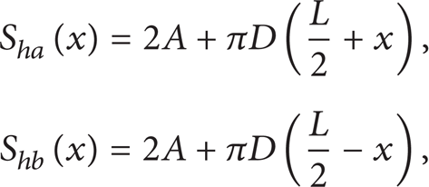
\begin{matrix} S_{h a} (x) = 2 A + π D (\frac{L}{2} + x), \\ S_{h b} (x) = 2 A + π D (\frac{L}{2} - x), \end{matrix}

(6)

where D is the diameter of piston.

Figure 2:

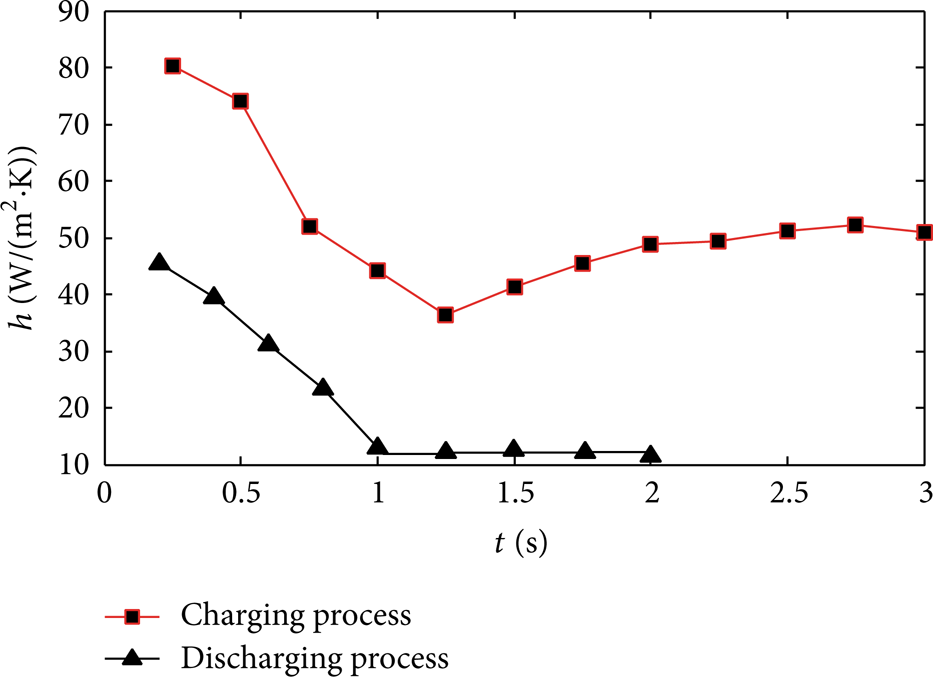
Measured values of heat transfer coefficient.

Neglecting the valve dynamics, a combination of the International Standards Organization (ISO) recommended model and the theoretical model of compressible flow through an orifice is used to describe the flow through the valve MPYE-5-1/8-HF-010B; consider the following:

\dot{m} = {\begin{cases} A (u) C_{d} C_{1} \frac{p_{u}}{\sqrt{T_{u}}}, & \frac{p_{d}}{p_{u}} \leq p_{r}, \\ A (u) C_{d} C_{1} \frac{p_{u}}{\sqrt{T_{u}}} \sqrt{1 - {(\frac{p_{d} / p_{u} - p_{r}}{1 - p_{r}})}^{2}}, & \frac{p_{d}}{p_{u}} > p_{r}, \end{cases}

(7)

where $\dot{m}$ is the mass flow rate, A(u) is the effective valve orifice area, C_d is the discharge coefficient, p_u and p_d are the upstream pressure and the downstream pressure, respectively, T_u is the upstream temperature of air, p_r is the critical pressure ratio, and C₁ is a constant calculated by

C_{1} = \sqrt{\frac{γ}{R} {(\frac{2}{γ + 1})}^{(γ + 1) / (γ - 1)}} = 0.0404 .

(8)

To reduce the complexity of the model, the critical pressure ratio p_r is assumed to take a constant value of 0.29 according to the valve catalogue. Since it has been confirmed experimentally that the valve is approximately symmetrical but unmatched, through measuring the mass flow rate under different input signals and work port pressures, the relation between input signal u and orifice area (input and exhaust paths) could be obtained as shown in Figure 3. Note that the valve null voltage is not 5 V as expected. The discharge coefficient C_d is introduced to account for flow reduction caused by contraction and losses. It depends on the pressure ratio and is identified experimentally as follows:

C_{d} = 0.8153 + 0.0933 (\frac{p_{d}}{p_{u}}) - 0.1038 {(\frac{p_{d}}{p_{u}})}^{2} .

(9)

Figure 3:

Input and exhaust path valve areas versus input signal.

Generally, the system is subjected to parametric uncertainties due to the variation of b, A_f, F_L, h, and so forth and uncertain nonlinearities represented by $\tilde{f}$ , ${\tilde{d}}_{a}$ , and ${\tilde{d}}_{b}$ . In practical, uncertain nonlinearities may be divided into two components: the slowly changing part denoted by f_n, d_an, and d_bn and the fast changing part denoted by ${\tilde{f}}_{0}$ , ${\tilde{d}}_{a 0}$ , and ${\tilde{d}}_{b 0}$ . The slowly changing part f_n, d_an, and d_bn together with other important unknown parameters can be updated online through adaption law for an improved performance. To achieve this, define the parameter set $θ = {[θ_{1}, θ_{2}, θ_{3}, θ_{4}, θ_{5}]}^{T}$ as θ₁ = b, θ₂ = A_f, θ₃ = −F_L + f_n, θ₄ = d_an, and θ₅ = d_bn. In order to minimize the numerical error and facilitate the gain-tuning process, a constant scaling factor S_p = 10⁵ is introduced to the chamber pressures; the scaled pressures are ${\bar{p}}_{a} = p_{a} / S_{p}$ and ${\bar{p}}_{b} = p_{b} / S_{p}$ . Define the state variables $x = {[x_{1}, x_{2}, x_{3}, x_{4}]}^{T} = {[x, \dot{x}, {\bar{p}}_{a}, {\bar{p}}_{b}]}^{T}$ , and the entire system dynamics can be written in a state-space form as

\begin{matrix} {\dot{x}}_{1} = x_{2}, \\ m {\dot{x}}_{2} = \bar{A} (x_{3} - x_{4}) - θ_{1} x_{2} - θ_{2} S_{f} (x_{2}) + θ_{3} + {\tilde{f}}_{0}, \\ {\dot{x}}_{3} = \frac{γ R}{S_{p} V_{a}} ({\dot{m}}_{a in} T_{s} - {\dot{m}}_{a out} T_{a}) - \frac{γ A}{V_{a}} x_{2} x_{3} + \frac{(γ - 1)}{S_{p} V_{a}} {\dot{Q}}_{a} + θ_{4} + {\tilde{d}}_{a 0}, \\ {\dot{x}}_{4} = \frac{γ R}{S_{p} V_{b}} ({\dot{m}}_{b in} T_{s} - {\dot{m}}_{b out} T_{b}) + \frac{γ A}{V_{b}} x_{2} x_{4} + \frac{(γ - 1)}{S_{p} V_{b}} {\dot{Q}}_{b} + θ_{5} + {\tilde{d}}_{b 0}, \end{matrix}

(10)

where $\bar{A} = A S_{p}$ . Since the extent of parametric uncertainties and modeling errors can be predicted, the following assumption is made.

Assumption 1. The extent of parametric uncertainties and uncertain nonlinearities are known; that is,

\begin{matrix} θ \in Ω_{θ} = {θ : θ_{\min} \leq θ \leq θ_{\max}}, \\ | {\tilde{f}}_{0} (t) | \leq f_{\max}, | {\tilde{d}}_{a 0} (t) | \leq d_{a \max}, \\ | {\tilde{d}}_{b 0} (t) | \leq d_{b \max}, \end{matrix}

(11)

where $θ_{\min} = {[\begin{bmatrix} θ_{1 \min} & θ_{2 \min} & θ_{3 \min} & θ_{4 \min} & θ_{5 \min} \end{bmatrix}]}^{T}$ and θ_max⁡ = [θ_1max θ_2max θ_3max θ_4max θ_5max]^T are the minimum parameter vector and the maximum parameter vector, respectively, and f_max, d_amax, and d_bmax are known scalars.

For simplicity, the following notations are used throughout the paper: •_i is used for the ith component of the vector •, the operation ≤ for two vectors is performed in terms of the corresponding elements of the vectors, $\hat{•}$ is used to denote the estimate of •, and $\tilde{•}$ is used to denote the estimation error; that is, $\tilde{•} = \hat{•} - •$ .

The control objective is to synthesize a control input u for system (10) such that x₁ tracks the desired trajectory x_1d with a guaranteed transient and final tracking accuracy. The desired trajectory x_1d is assumed to be known, bounded with bounded derivatives up to the second order. Since the model uncertainties are unmatched in system (10), the recursive backstepping design technique will be employed. Two popular nonlinear control tools, robust backstepping control and tuning function based adaptive backstepping control, will be applied first, from which one can gain insights into the development and the advantages of the adaptive robust control.

3. Controller Design

3.1. Tuning Function Based Adaptive Backstepping Control

Step 1. Assuming that the system has parametric uncertainties only, $that is, {\tilde{f}}_{0} = {\tilde{d}}_{a 0} = {\tilde{d}}_{b 0} = 0$ in (10), let e₁ = x₁-x_1d be the trajectory tracking error, defining a switch-function-like quantity as

e_{2} = {\dot{e}}_{1} + k_{1} e_{1} = x_{2} - x_{2 eq}, x_{2 eq} ≜ {\dot{x}}_{1 d} - k_{1} e_{1},

(12)

where k₁ is a positive feedback gain. Since the transfer function from e2 to e1, that is, $G_{e_{1} e_{2}} (s) = 1 / (s + k_{1})$ is stable, making e₂ converge to a small value or zero is equivalent to making e1 converge to a small value or zero. Differentiating e2 and substituting it into the second equation of (10) leads to

m {\dot{e}}_{2} = \bar{A} (x_{3} - x_{4}) - θ_{1} x_{2} - θ_{2} S_{f} (x_{2}) + θ_{3} - m {\dot{x}}_{2 eq} .

(13)

Let p_L = x₃-x₄ denote the scaled pressure difference between two chambers. Considering p_L as the virtual control input, the adaptive control law p_Ld for p_L is then given by

\begin{matrix} p_{L d} = p_{L d a} + p_{L d s}, \\ p_{L d a} = \frac{1}{\bar{A}} [{\hat{θ}}_{1} x_{2} + {\hat{θ}}_{2} S_{f} (x_{2}) - {\hat{θ}}_{3} + m {\dot{x}}_{2 eq}], \\ p_{L d s} = - \frac{1}{\bar{A}} k_{2} e_{2}, k_{2} > 0, \end{matrix}

(14)

where p_Lda is the model compensation term with online parameter estimates ${\hat{θ}}_{1}$ , ${\hat{θ}}_{2}$ , and ${\hat{θ}}_{3}$ and p_Lds is the robust feedback term, which is chosen to be a simple proportional feedback of e₂. Let e₃ = p_L-p_Ld denote the virtual control input discrepancy.

Define a positive semidefinite function

V_{2} = \frac{1}{2} m e_{2}^{2} + \frac{1}{2} {\tilde{θ}}^{T} Γ^{- 1} \tilde{θ},

(15)

where Γ is the positive definite symmetric adaption rate matrix. Differentiating V₂ and substituting (13) and (14) into it yields

{\dot{V}}_{2} = \bar{A} e_{3} e_{2} - k_{2} e_{2}^{2} + {\tilde{θ}}^{T} Γ^{- 1} (\dot{\tilde{θ}} - Γ ϕ_{2} e_{2}),

(16)

where $ϕ_{2} = {[- x_{2}, - S_{f} (x_{2}), 1,0, 0]}^{T}$ is the first regressor vector. Therefore, the first tuning function can be defined as τ₂ = ϕ₂e₂ [25].

Step 2. Differentiating e₃ and substituting the last two equations of (10) into it yields

\begin{matrix} {\dot{e}}_{3} = q_{L} - (\frac{γ A}{V_{a}} x_{2} x_{3} + \frac{γ A}{V_{b}} x_{2} x_{4}) + \frac{(γ - 1)}{S_{p} V_{a}} {\dot{Q}}_{a} - \frac{(γ - 1)}{S_{p} V_{b}} {\dot{Q}}_{b} + θ_{4} - θ_{5} - {\dot{p}}_{L d c} - {\dot{p}}_{L d u}, \\ q_{L} = \frac{γ R}{S_{p} V_{a}} ({\dot{m}}_{a in} T_{s} - {\dot{m}}_{a out} T_{a}) - \frac{γ R}{S_{p} V_{b}} ({\dot{m}}_{b in} T_{s} - {\dot{m}}_{b out} T_{b}), \\ {\dot{p}}_{L d c} = \frac{\partial p_{L d}}{\partial x_{1}} x_{2} + \frac{\partial p_{L d}}{\partial x_{2}} {\hat{\dot{x}}}_{2} + \frac{\partial p_{L d}}{\partial \hat{θ}} Γ τ_{2}, \\ {\hat{\dot{x}}}_{2} = \frac{1}{m} [\bar{A} (x_{3} - x_{4}) - {\hat{θ}}_{1} x_{2} - {\hat{θ}}_{2} S_{f} (x_{2}) + {\hat{θ}}_{3}], \\ {\dot{p}}_{L d u} = \frac{1}{m} \frac{\partial p_{L d}}{\partial x_{2}} [{\tilde{θ}}_{1} x_{2} + {\tilde{θ}}_{2} S_{f} (x_{2}) - {\tilde{θ}}_{3}] + \frac{\partial p_{L d}}{\partial \hat{θ}} (\dot{\hat{θ}} - Γ τ_{2}) . \end{matrix}

(17)

Consider q_L as the virtual control input. Therefore, next is to synthesize a control function q_Ld for q_L such that the (e₂,e₃) system ((13) and (17)) is stable with respect to

V_{3} = V_{2} + \frac{1}{2} e_{3}^{2} .

(18)

Similar to (14), the following virtual control function q_Ld is proposed:

\begin{matrix} q_{L d} = q_{L d a} + q_{L d s}, \\ q_{L d a} = - \bar{A} e_{2} + (\frac{γ A}{V_{a}} x_{2} x_{3} + \frac{γ A}{V_{b}} x_{2} x_{4}) - \frac{(γ - 1)}{S_{p} V_{a}} {\dot{Q}}_{a} + \frac{(γ - 1)}{S_{p} V_{b}} {\dot{Q}}_{b} - {\hat{θ}}_{4} + {\hat{θ}}_{5} + {\dot{p}}_{L d c} + ν, \\ q_{L d s} = - k_{3} e_{3}, k_{3} > 0, \end{matrix}

(19)

where ν is a correction term yet to be chosen. Since the effects of inexact mass flow rate model equation (7) were lumped into modeling errors represented by ${\tilde{d}}_{a}$ and ${\tilde{d}}_{b}$ , let us suppose that there is no discrepancy between q_Ld and q_L. Differentiating V₃ and substituting (17) and (19) into it gives

{\dot{V}}_{3} = - k_{2} e_{2}^{2} - k_{3} e_{3}^{2} + e_{3} (ν - \frac{\partial p_{L d}}{\partial \hat{θ}} Γ ϕ_{3} e_{3}) - e_{3} \frac{\partial p_{L d}}{\partial \hat{θ}} (\dot{\hat{θ}} - Γ τ_{3}) + {\tilde{θ}}^{T} Γ^{- 1} (\dot{\tilde{θ}} - Γ τ_{3}),

(20)

where $ϕ_{3} = [(1 / m) (\partial p_{L d} / \partial x_{2}) x_{2}$ , $(1 / m) (\partial p_{L d} / \partial x_{2}) S_{f} (x_{2})$ , $- (1 / m) (\partial p_{L d} / \partial x_{2}), 1, - 1] T$ is the second regressor vector and τ₃ = τ₂ + ϕ₃e₃ is the second tuning function [25]. From (20), the choice of ν is immediate. Consider

ν = \frac{\partial p_{L d}}{\partial \hat{θ}} Γ ϕ_{3} e_{3} .

(21)

To eliminate $\tilde{θ}$ from ${\dot{V}}_{3}$ , the parameter adaption law is chosen as

\dot{\hat{θ}} = Γ τ_{3} .

(22)

Finally, the resulting ${\dot{V}}_{3}$ is

{\dot{V}}_{3} = - k_{2} e_{2}^{2} - k_{3} e_{3}^{2} .

(23)

Therefore, all signals in the system are bounded and the tracking error asymptotically converges to zero.

Step 3. Once the q_Ld is calculated according to (19), the input signal u for the proportional directional control valve could be obtained according to (7) and the relation between the input signal and effective valve orifice area (see Figure 3).

3.2. Deterministic Robust Control

Deterministic robust control utilizes nonlinear feedback to overpower both types of model uncertainty effects; its design parallels the adaptive backstepping design in the above subsection.

Step 1. When the uncertain nonlinearities exist, rewrite the derivative of e₂ as

m {\dot{e}}_{2} = \bar{A} (x_{3} - x_{4}) - θ_{1} x_{2} - θ_{2} S_{f} (x_{2}) + θ_{3} + {\tilde{f}}_{0} - m {\dot{x}}_{2 eq} .

(24)

The robust control law p_Ld for p_L is given by

\begin{matrix} p_{L d} = p_{L d a} + p_{L d s 1} + p_{L d s 2}, \\ p_{L d a} = \frac{1}{\bar{A}} [{\hat{θ}}_{10} x_{2} + {\hat{θ}}_{20} S_{f} (x_{2}) - {\hat{θ}}_{30} + m {\dot{x}}_{2 eq}], \\ p_{L d s 1} = - \frac{1}{\bar{A}} k_{2} e_{2}, k_{2} > 0, \end{matrix}

(25)

where p_Lda has the same form as that in (14) except that ${\hat{θ}}_{i 0}$ is the offline estimated value of θ_i, p_Lds1 is used to stabilize the nominal system, which is chosen to be a simple proportional feedback of e₂, and p_Lds2 is a robust feedback term to be synthesized later so that some guaranteed robust performance can be achieved in spite of various model uncertainties. Define a different positive semidefinite function

V_{2} = \frac{1}{2} m e_{2}^{2} .

(26)

Differentiating V₂ and substituting (24) and (25) into it yields

\begin{matrix} {\dot{V}}_{2} = \bar{A} e_{3} e_{2} - k_{2} e_{2}^{2} \\ + e_{2} [\bar{A} p_{L d s 2} + {\tilde{θ}}_{10} x_{2} + {\tilde{θ}}_{20} S_{f} (x_{2}) - {\tilde{θ}}_{30} + {\tilde{f}}_{0}] \\ = \bar{A} e_{3} e_{2} + {{\dot{V}}_{2} |}_{p_{L d}}, \end{matrix}

(27)

where ${{\dot{V}}_{2} |}_{p_{L d}}$ is a short-hand notation used to represent ${\dot{V}}_{2}$ when p_L = p_Ld; that is, e₃ = 0. By assumption, the last four terms inside the brackets of (27) are bounded above with some known functions h₂(t). For example, h₂(t) can be chosen as

h_{2} (t) = | θ_{M 1} | | x_{2} | + | θ_{M 2} | | S_{f} (x_{2}) | + | θ_{M 3} | + f_{\max},

(28)

where θ_Mi = θ_imax – θ_imin, i = 1, 2, 3. Using the smoothed sliding mode control technology, the robust control function p_Lds2 can be chosen as

p_{L d s 2} = - \frac{h_{2}^{2} (t)}{4 η_{2} \bar{A}} e_{2},

(29)

where η₂>0 is a design parameter and can be considered as the boundary layer thickness. Thus, the following conditions are satisfied:

e_{2} [\bar{A} p_{L d s 2} + {\tilde{θ}}_{10} x_{2} + {\tilde{θ}}_{20} S_{f} (x_{2}) - {\tilde{θ}}_{30} + {\tilde{f}}_{0}] \leq η_{2} .

(30)

Substituting (30) into (27) leads to

{\dot{V}}_{2} \leq \bar{A} e_{3} e_{2} - k_{2} e_{2}^{2} + η_{2} .

(31)

Step 2. As seen from (31), if e₃ = 0, then e2 will exponentially converge to the ball whose size can be made arbitrarily small by increasing feedback gain k2 and/or decreasing controller parameter η₂. Therefore, next is to synthesize a virtual control function such that e3 converges to zero or a small value with a guaranteed transient performance. In the presence of uncertain nonlinearities ${\tilde{f}}_{0}$ , ${\tilde{d}}_{a 0}$ , and ${\tilde{d}}_{b 0}$ , the derivative of e3 can be rewritten as

\begin{matrix} {\dot{e}}_{3} = q_{L} - (\frac{γ A}{V_{a}} x_{2} x_{3} + \frac{γ A}{V_{b}} x_{2} x_{4}) + \frac{(γ - 1)}{S_{p} V_{a}} {\dot{Q}}_{a} - \frac{(γ - 1)}{S_{p} V_{b}} {\dot{Q}}_{b} + θ_{4} - θ_{5} + {\tilde{d}}_{a 0} - {\tilde{d}}_{b 0} - {\dot{p}}_{L d c} - {\dot{p}}_{L d u}, \\ q_{L} = \frac{γ R}{S_{p} V_{a}} ({\dot{m}}_{a in} T_{s} - {\dot{m}}_{a out} T_{a}) - \frac{γ R}{S_{p} V_{b}} ({\dot{m}}_{b in} T_{s} - {\dot{m}}_{b out} T_{b}), \\ {\dot{p}}_{L d c} = \frac{\partial p_{L d}}{\partial x_{1}} x_{2} + \frac{1}{m} \frac{\partial p_{L d}}{\partial x_{2}} [\bar{A} (x_{3} - x_{4}) - {\hat{θ}}_{10} x_{2} - {\hat{θ}}_{20} S_{f} (x_{2}) + {\hat{θ}}_{30}], \\ {\dot{p}}_{L d u} = \frac{1}{m} \frac{\partial p_{L d}}{\partial x_{2}} [{\tilde{θ}}_{1} x_{2} + {\tilde{θ}}_{2} S_{f} (x_{2}) - {\tilde{θ}}_{3} + {\tilde{f}}_{0}], \end{matrix}

(32)

where ${\dot{p}}_{L d c}$ represents the calculable part of ${\dot{p}}_{L d}$ and can be used to design control functions, while ${\dot{p}}_{L d u}$ is the incalculable part due to various uncertainties and has to be dealt with by certain robust feedback as in Step 1.

Consider q_L as the virtual control input. Similar to (25), the following robust control function q_Ld is proposed:

\begin{matrix} q_{L d} = q_{L d a} + q_{L d s 1} + q_{L d s 2}, \\ q_{L d a} = - \bar{A} e_{2} + (\frac{γ A}{V_{a}} x_{2} x_{3} + \frac{γ A}{V_{b}} x_{2} x_{4}) - \frac{(γ - 1)}{S_{p} V_{a}} {\dot{Q}}_{a} + \frac{(γ - 1)}{S_{p} V_{b}} {\dot{Q}}_{b} - {\hat{θ}}_{40} + {\hat{θ}}_{50} + {\dot{p}}_{L d c}, \\ q_{L d s 1} = - k_{3} e_{3}, k_{3} > 0 . \end{matrix}

(33)

Define a positive semidefinite function

V_{3} = V_{2} + \frac{1}{2} e_{3}^{2} .

(34)

Differentiating V₃ and substituting (27), (32), and (33) into it gives

\begin{matrix} {\dot{V}}_{3} = {{\dot{V}}_{2} |}_{p_{L d}} - k_{3} e_{3}^{2} + e_{3} [q_{L d s 2} - {\tilde{θ}}_{40} + {\tilde{θ}}_{50} + {\tilde{d}}_{a 0} - {\tilde{d}}_{b 0} - {\dot{p}}_{L d u}] . \end{matrix}

(35)

As in Step 1, q_Lds2 is chosen as

\begin{matrix} q_{L d s 2} = - \frac{h_{3}^{2} (t)}{4 η_{3}} e_{3}, η_{3} > 0 \\ , \\ h_{3} (t) = | \frac{1}{m} \frac{\partial p_{L d}}{\partial x_{2}} | \times [| θ_{M 1} | | x_{2} | + | θ_{M 2} | | S_{f} (x_{2}) | + | θ_{M 3} | + f_{\max}] + | θ_{M 4} | + | θ_{M 5} | + d_{a \max} + d_{b \max} . \end{matrix}

(36)

Therefore, the following condition is satisfied:

e_{3} [q_{L d s 2} - {\tilde{θ}}_{40} + {\tilde{θ}}_{50} + {\tilde{d}}_{a 0} - {\tilde{d}}_{b 0} - {\dot{p}}_{L d u}] \leq η_{3} .

(37)

Substituting (37) into (35) and noting (31) leads to

{\dot{V}}_{3} \leq - k_{2} e_{2}^{2} - k_{3} e_{3}^{2} + η_{2} + η_{3} \leq - λ V_{3} + η,

(38)

where $λ = \min {2 k_{2} / m, 2 k_{3}}$ and η = η₂ + η₃. Thus, the error vector $e = {[e_{2}, e_{3}]}^{T}$ is bounded above by

{∥ e (t) ∥}^{2} \leq e^{- λ t} ∥ e (0) ∥ + \frac{2 η}{λ} (1 - e^{- λ t}) .

(39)

Hence, e₂ and e₃ will exponentially converge to some balls whose sizes can be adjusted via parameters k₂, k₃, η₂, and η₃, and thus e₁ is ultimately bounded.

Step 3. Once the q_Ld is calculated according to (33) and (36), the input signal u for the proportional directional control valve could be obtained according to (7) and the relation between the input signal and effective valve orifice area (see Figure 3).

3.3. Adaptive Robust Control

The ARC law has a similar structure as the robust backstepping control law except that an online estimate of θ is used to further improve the steady-state tracking performance. However, the adaption law like (22) cannot directly be adopted in the ARC since it could lead to unbounded parameter estimates in the presence of disturbance. Thus, no bounded robust control term p_Lds2 and term q_Lds2 can be founded to attenuate the unbounded model uncertainties in (25) and (33), respectively. As a result, the widely used projection mapping in adaptive control will be used to condition the online parameter estimation algorithm so that the parameter estimates are kept within the known bounded convex set ${\bar{Ω}}_{θ}$ , the closure of the convex set Ω_θ. Furthermore, in order to achieve a complete separation of estimator design and robust control design, in addition to the projection mapping, it is also necessary to use the preset adaption rate limits for a controlled estimation process. Therefore, the parameter estimate $\hat{θ}$ is updated using the following projection type algorithm with a preset adaption rate limit ${\dot{θ}}_{M}$ . Consider

\dot{\hat{θ}} = sa t_{{\dot{θ}}_{M}} (Pro j_{\hat{θ}} (Γ τ)),

(40)

where τ is the adaption function, Γ is the positive definite symmetric adaption rate matrix, $Pro j_{\hat{θ}} (Γ τ)$ is the standard projection mapping, and $sa t_{{\dot{θ}}_{M}} (•)$ is the saturation function.

The standard projection mapping is

Pro j_{\hat{θ}} (Γ τ) = {\begin{cases} Γ τ, & if \hat{θ} \in {\overset{\circ}{Ω}}_{θ} or n_{\hat{θ}}^{T} Γ τ \leq 0, \\ (1 - Γ \frac{n_{\hat{θ}} n_{\hat{θ}}^{T}}{n_{\hat{θ}}^{T} Γ n_{\hat{θ}}}) Γ τ, & if \hat{θ} \in \partial Ω_{θ} or n_{\hat{θ}}^{T} Γ τ > 0, \end{cases}

(41)

where ${\overset{\circ}{Ω}}_{θ}$ and ∂Ω_θ denote the interior and the boundary of Ω_θ, respectively, and $n_{\hat{θ}}$ represents the outward unit normal vector at $\hat{θ} \in \partial Ω_{θ}$ .

The saturation function is defined as

sa t_{{\dot{θ}}_{M}} (•) = s_{0} •, s_{0} = {\begin{cases} 1, & ∥ • ∥ \leq {\dot{θ}}_{M}, \\ \frac{{\dot{θ}}_{M}}{∥ • ∥}, & ∥ • ∥ > {\dot{θ}}_{M}, \end{cases}

(42)

where ${\dot{θ}}_{M}$ is the preset adaption rate limit.

It has been proven in [28] that for any adaption function τ to be used such a parameter adaption law guarantees that the parameter estimates and their derivatives are bounded with known bounds. That is, the following properties will be held and a complete separation of the robust control law design from the parameter adaption process is realized:

\begin{matrix} \hat{θ} (t) \in {\bar{Ω}}_{θ} = {\hat{θ} : θ_{\min} \leq \hat{θ} \leq θ_{\max}}, \forall t, \\ {\tilde{θ}}^{T} [Γ^{- 1} Pro j_{\hat{θ}} (Γ τ) - τ] \leq 0, \forall τ, \\ | \dot{\hat{θ}} (t) | \leq {\dot{θ}}_{M}, \forall t . \end{matrix}

(43)

To achieve better convergence of parameter estimates, recursive least squares estimation algorithm with exponential forgetting factor and covariance resetting is applied to obtain the adaption function τ and the adaption rate matrix Γ in (40). For this purpose, it is assumed that the system is free of uncertain nonlinearities; $that is, {\tilde{f}}_{0} = {\tilde{d}}_{a 0} = {\tilde{d}}_{b 0} = 0$ in (10). Let H_f(s) be a stable LTI filter transfer function with a relative degree 3; for example,

H_{f} (s) = \frac{ω_{f}^{2}}{(τ_{f} s + 1) (s^{2} + 2 ξ ω_{f} s + ω_{f}^{2})},

(44)

where τ_f, ω_f, and ξ are filter parameters. Applying the filter to both sides of the last three equations of (10) and rewriting these equations, the following filtered line regression models can be constructed:

\begin{matrix} y_{1 f} = H_{f} [\bar{A} (x_{3} - x_{4}) - m {\dot{x}}_{2}] = θ_{1} x_{2 f} + θ_{2} S_{f f} (x_{2}) - θ_{3} 1_{f}, \\ y_{2 f} = H_{f} [\frac{γ R}{S_{p} V_{a}} ({\dot{m}}_{a in} T_{s} - {\dot{m}}_{a out} T_{a}) - \frac{γ A}{V_{a}} x_{2} x_{3} + \frac{(γ - 1)}{S_{p} V_{a}} {\dot{Q}}_{a}] = - θ_{4} 1_{f}, \\ y_{3 f} = H_{f} [\frac{γ R}{S_{p} V_{b}} ({\dot{m}}_{b in} T_{s} - {\dot{m}}_{b out} T_{b}) + \frac{γ A}{V_{b}} x_{2} x_{4} + \frac{(γ - 1)}{S_{p} V_{b}} {\dot{Q}}_{b}] = - θ_{5} 1_{f}, \end{matrix}

(45)

where x_2f, $S_{f f} (x_{2})$ , and 1_f represent the output of the filter H_f(s) for the input x₂, $S_{f} (x_{2})$ , and 1, respectively. Dividing parameter vector θ into three subsets $θ_{1 s} = {[θ_{1}, θ_{2}, θ_{3}]}^{T}$ , $θ_{2 s} = {[θ_{4}]}^{T}$ , and $θ_{3 s} = {[θ_{5}]}^{T}$ , (45) can be written in the form of standard linear regression model as follows:

y_{i f} = φ_{i f}^{T} θ_{i s}, i = 1,2, 3,

(46)

where φif represents the regressors; that is, $φ_{1 f}^{T} = [x_{2 f}, S_{f f} (x_{2}), - 1_{f}]$ , $φ_{2 f}^{T} = [- 1_{f}]$ , and $φ_{3 f}^{T} = [- 1_{f}]$ . Defining the predicted output as ${\hat{y}}_{i f} = φ_{i f}^{T} {\hat{θ}}_{i s}$ leads to the following prediction error model:

ε_{i} = {\hat{y}}_{i f} - y_{i f} = φ_{i f}^{T} {\tilde{θ}}_{i s}, i = 1,2, 3 .

(47)

Therefore, for each set of regressors and corresponding unknown parameter vectors, the adaption rate matrix is given by

{\dot{Γ}}_{i} = {\begin{cases} α_{i} Γ_{i} - \frac{Γ_{i} φ_{i f} φ_{i f}^{T} Γ_{i}}{1 + ν_{i} φ_{i f}^{T} Γ_{i} φ_{i f}}, \\ if λ_{\max} (Γ_{i} (t)) \leq ρ_{M}, ∥ Pro j_{{\hat{θ}}_{i}} (Γ_{i} τ_{i}) ∥ \leq {\dot{θ}}_{M}, \\ 0, \\ otherwise, \end{cases}

(48)

where α_i≥0 is the forgetting factor, ν_i≥0 is the normalizing factor with ν_i = 0 leading to the unnormalized algorithm, ρ_M is the preset upper bound for $∥ Γ_{i} (t) ∥$ which guarantees Γ_i(t) ≤ ρ_MI,∀t, and the adaption function τ_i is defined as

τ_{i} = \frac{1}{1 + ν_{i} φ_{i f}^{T} Γ_{i} φ_{i f}} φ_{i f} ε_{i} .

(49)

The ARC and robust backstepping control laws share the same structure except that an online estimate of θ as described above, instead of the fixed offline estimate, is used. Thus, the adaptive robust control law p_Ld for p_L is given by

\begin{matrix} p_{L d} = p_{L d a} + p_{L d s 1} + p_{L d s 2}, \\ p_{L d a} = \frac{1}{\bar{A}} [{\hat{θ}}_{1} x_{2} + {\hat{θ}}_{2} S_{f} (x_{2}) - {\hat{θ}}_{3} + m {\dot{x}}_{2 eq}], \\ p_{L d s 1} = - \frac{1}{\bar{A}} k_{2} e_{2}, k_{2} > 0, \\ p_{L d s 2} = - \frac{h_{2}^{2} (t)}{4 η_{2} \bar{A}} e_{2}, η_{2} > 0, \\ h_{2} (t) = | θ_{M 1} | | x_{2} | + | θ_{M 2} | | S_{f} (x_{2}) | + | θ_{M 3} | + f_{\max} . \end{matrix}

(50)

Similar to (33), the following adaptive robust control function q_Ld for q_L is proposed:

\begin{matrix} q_{L d} = q_{L d a} + q_{L d s}, q_{L d s} = q_{L d s 1} + q_{L d s 2}, \\ q_{L d a} = - \bar{A} e_{2} + (\frac{γ A}{V_{a}} x_{2} x_{3} + \frac{γ A}{V_{b}} x_{2} x_{4}) - \frac{(γ - 1)}{S_{p} V_{a}} {\dot{Q}}_{a} + \frac{(γ - 1)}{S_{p} V_{b}} {\dot{Q}}_{b} - {\hat{θ}}_{4} + {\hat{θ}}_{5} + {\dot{p}}_{L d c}, \\ {\dot{p}}_{L d c} = \frac{\partial p_{L d}}{\partial x_{1}} x_{2} + \frac{\partial p_{L d}}{\partial x_{2}} {\hat{\dot{x}}}_{2} + \frac{\partial p_{L d}}{\partial \hat{θ}} \dot{\hat{θ}}, \\ {\hat{\dot{x}}}_{2} = \frac{1}{m} [\bar{A} (x_{3} - x_{4}) - {\hat{θ}}_{1} x_{2} - {\hat{θ}}_{2} S_{f} (x_{2}) + {\hat{θ}}_{3}], \\ q_{L d s 1} = - k_{3} e_{3}, k_{3} > 0, \\ q_{L d s 2} = - \frac{h_{3}^{2} (t)}{4 η_{3}} e_{3}, η_{3} > 0, \\ h_{3} (t) = | \frac{1}{m} \frac{\partial p_{L d}}{\partial x_{2}} | \times [| θ_{M 1} | | x_{2} | + | θ_{M 2} | | S_{f} (x_{2}) | + | θ_{M 3} | + f_{\max}] + | θ_{M 4} | + | θ_{M 5} | + d_{a \max} + d_{b \max} . \end{matrix}

(51)

Once the q_Ld is calculated according to (51), the input signal u for the proportional directional control valve could be obtained according to (7) and the relation between the input signal and effective valve orifice area (see Figure 3).

Remark. The system has one-dimensional internal dynamics, which arises from the physical phenomenon that there are infinite number pairs of (p_a, p_b) to produce the desired virtual control input p_L. Rigorous theoretical proof of the stability of the internal dynamics is very hard and will be one of the focuses of our future work. Nevertheless, extensive experimental results obtained in this paper do prove that the two chamber pressures are bounded; that is, the internal dynamics is indeed stable.

4. Experimental Results

To test the proposed control strategy, an experimental setup has been built in our laboratory. The schematic of the experimental setup is shown in Figure 4. Figure 5 is the picture of the experimental setup. The cylinder (FESTO DGC-25-500-G-PPV-A) is controlled by a proportional directional control valve (FESTO MPYE-5-1/8-HF-010B). Pressure sensors (FESTO SDET-22T-D10-G14-I-M12) are used to measure the chamber pressures and the tank pressure. Position and velocity information of the cylinder movement is obtained by the magnetostrictive linear position sensor (MTS RPS0500MD601V810050). The control algorithms are implemented using a dSPACE DS1103 controller board, while an industrial computer is used as the user interface. The controller executes programs at a sampling period of 1 ms.

Figure 4:

Schematic representation of the experimental setup.

Figure 5:

Picture of the experimental setup.

The system physical parameters are m = 1.88 Kg, A = 4.908 × 10⁻⁴ m², L = 0.5 m, V_0a = 2.5 × 10⁻⁵ m³, V_0b = 5 × 10⁻⁵ m³, R = 287 N·m/Kg·K, γ = 1.4, T_s = 300 K, and p_s = 7 × 10⁵ Pa. The nominal values of the uncertain parameters are set as θ₁ = 80 N·s/m, θ₂ = 60 N, θ₃ = 0 N, θ₄ = 0 Pa/s, and θ₅ = 0 Pa/s. The bounds of the parametric variations are chosen as $θ_{\min} = {[0,0, - 100, - 10^{6}, - 10^{6}]}^{T}$ and $θ_{\max} = {[300,250,100, 10^{6}, 10^{6}]}^{T}$ . The following control algorithms are tested for comparison.

(C1)

Tuning Function Based Adaptive Backstepping Controller. The control parameters are set as k₁ = 50, k₂ = 20, and k₃ = 200. The adaption rates are set as $Γ = diag {100,100,100,50,50}$ .

(C2)

Robust Backstepping Controller. The offline parameter estimates are chosen as ${\hat{θ}}_{0} = {[80,60,0, 0,0]}^{T}$ . After trial and error, the control gains adopted are k₁ = 45, k₂ = 30, h₂(t) = 100, η₂ = 4, k₃ = 200, h₃(t) = 400, and η₃ = 10.

(C3)

ARC Controller. The same control gains as those in (C2) are used. The initial values of the adaption rate matrices are set as $Γ_{1} (0) = diag {100,100,100}$ , $Γ_{2} (0) = 100$ , and $Γ_{3} (0) = 100$ . The filter parameters are τ_f = 50, ω_f = 100, and ξ = 1. Other parameters in parameter estimation algorithm are α₁ = α₂ = α₃ = 0.1, ν₁ = ν₂ = ν₃ = 0.1, ρ_M = 1000, and ${\dot{θ}}_{M} = {[10,10,10,10,10]}^{T}$ .

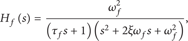
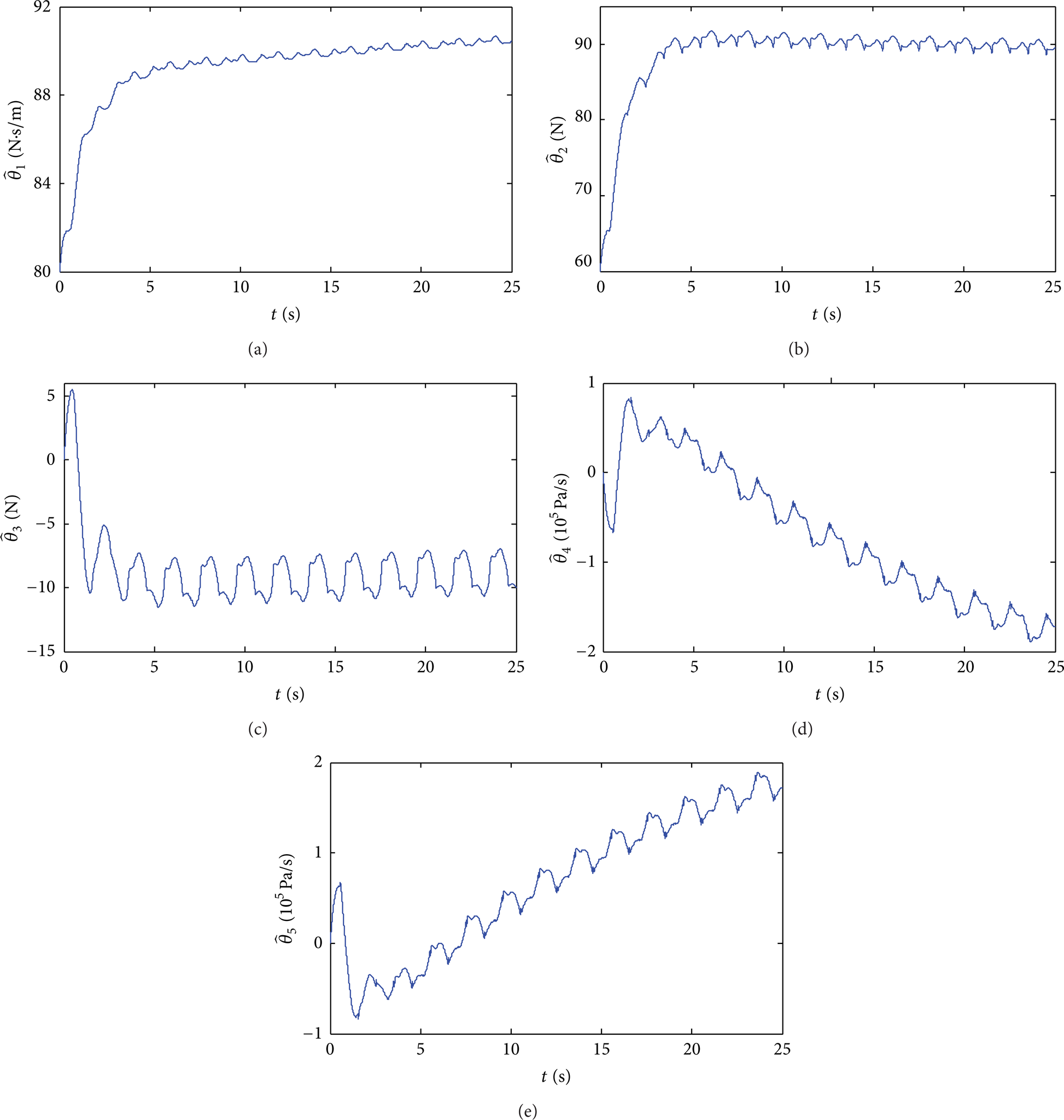
The effectiveness of the proposed controllers has been demonstrated by a number of comparative experiments. Some typical results are given below. The following performance indices will be used to quantify each control algorithm. (1) ${∥ e_{1} ∥}_{rms} = \sqrt{(1 / 10) \int_{T_{f} - 10}^{T_{f}} e_{1}^{2} d t}$ , the root-mean-square value of the tracking error during the last ten seconds, is used as a measure of average tracking performance, where T_f represents the total running time. (2) $e_{1 M} = ma x_{T_{f} - 10 \leq t \leq T_{f}} {| e_{1} |}$ , the maximum absolute value of the tracking error during the last ten seconds, is used as a measure of final tracking accuracy. (3) ${∥ u ∥}_{rms} = \sqrt{(1 / T_{f}) \int_{0}^{T_{f}} {(u - 4.8)}^{2} d t}$ , the average control input during the last ten seconds, is used to evaluate the amount of control effort of each algorithm.

The controllers are first tested for tracking a sinusoidal trajectory with a frequency of 0.5 Hz and an amplitude of 0.125 m. The tracking errors are given in Figure 6. Table 1 shows the experimental results in terms of performance indices. Due to the use of parameter adaption as shown in Figures 7 and 8, (C1) and (C3) have much better steady-state tracking performance than (C2). In (C1), the adaption control law and parameter adaption law are synthesized simultaneously to meet the sole objective of reducing the output tracking error. The choice of parameter adaption law is limited to the gradient type with actual tracking errors as driving signals. Since the actual tracking error in implementation is normally small, the parameter estimates do not converge to their true values. In contrast, (C3) utilizes projection type RLSE algorithm, which realizes a complete separation of the control law design from the parameter adaption process, and more accurate parameter estimates are obtained. As a result, (C3) achieves an even better steady-state tracking performance than (C1). The final tracking error of (C3) is e_1M = 2.9 mm, and the average tracking error of (C3) is ${∥ e_{1} ∥}_{rms} = 1.4$ mm, which illustrates the effectiveness of the proposed ARC controller. The control inputs of the three controllers are shown in Figure 9. All controllers use almost the same amount of control effort, and (C3) has a larger degree of control input chattering than (C2) and (C1). Nevertheless, the proposed adaptive robust controller (C3) demands much less amount of control effort than in [19, 29] to achieve such a good tracking performance. The chamber pressures of (C3) are shown in Figure 10, which are bounded during the whole tracking process as expected.

Table 1:

Experimental results in terms of performance indices.

m (kg)	Trajectory	C ₁			C ₂			C ₃
m (kg)	Trajectory	e_1M (mm)	${∥ e_{1} ∥}_{rms}$ (mm)	${∥ u ∥}_{rms}$ (V)	e_1M (mm)	${∥ e_{1} ∥}_{rms}$ (mm)	${∥ u ∥}_{rms}$ (V)	e_1M (mm)	${∥ e_{1} ∥}_{rms}$ (mm)	${∥ u ∥}_{rms}$ (V)

1.88	$0.125 \sin (π t)$	4.6	1.5	0.90	6.1	4.3	0.94	2.9	1.4	0.96
6.20	$0.125 \sin (π t)$	5.7	1.9	1.40	9.5	7.7	1.37	2.7	1.7	1.17

Figure 6:

Tracking errors for sinusoidal trajectory sinusoidal without load.

Figure 7:

Parameter estimation of (C1) for trajectory motion without load.

Figure 8:

Parameter estimation of (C3) for sinusoidal trajectory motion without load.

Figure 9:

Control inputs for sinusoidal trajectory without load.

Figure 10:

Chamber pressures of (C3) for sinusoidal trajectory motion without load.

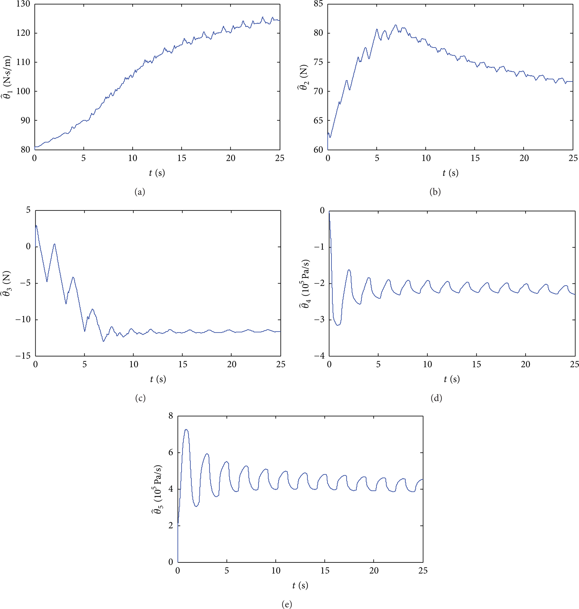
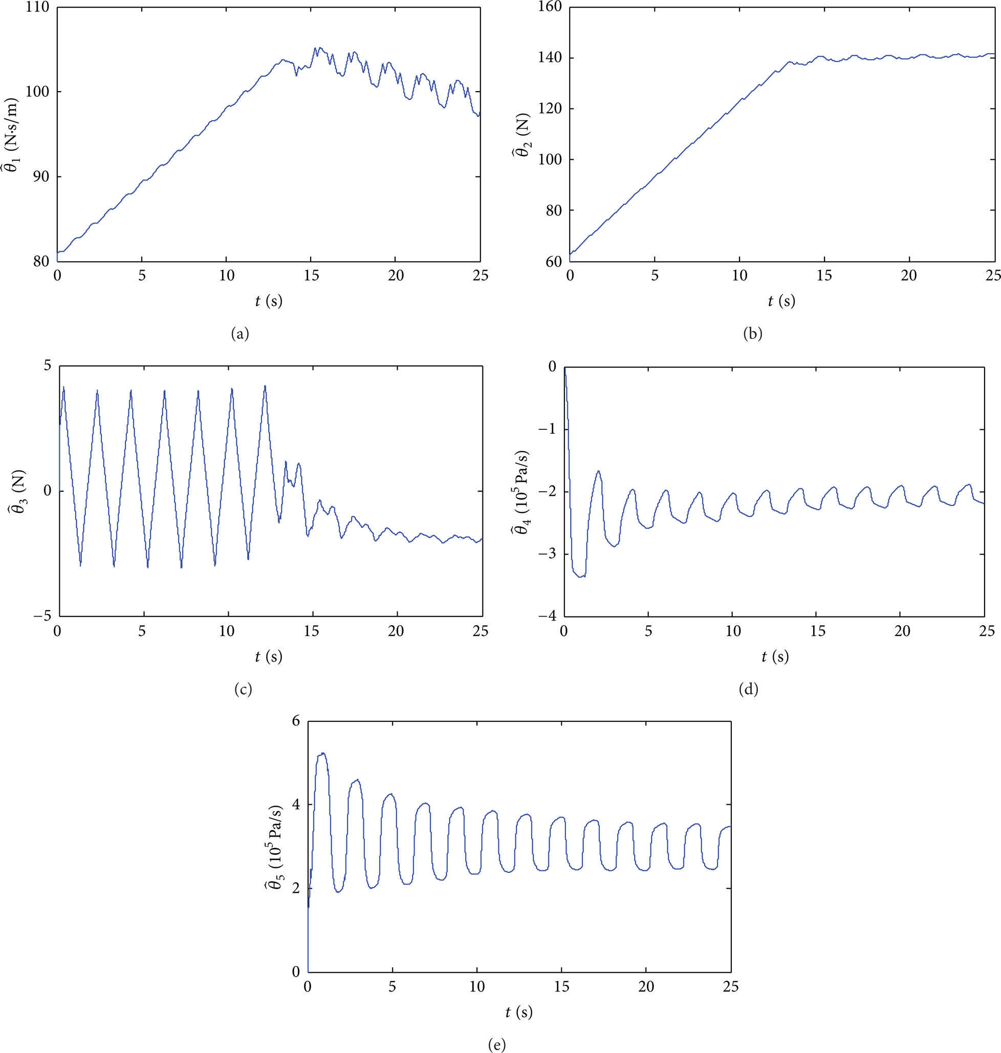
To test the performance robustness of the algorithms to the parameter variations, a 4.32 kg payload is mounted on the slide. The tracking errors are shown in Figure 11 and the experimental results in terms of performance indices are shown in Table 1. Figures 12 and 13 show the history of online parameter estimates of (C3) and (C1). Due to the change of payload, there exist large variations in the parameters. As seen, (C3) and (C1) perform much better than (C2). Although there are slightly large transient tracking errors, (C3) achieves almost the same steady-state tracking performance as before. This indicates that (C3) has high performance robustness to parameter variations. The control inputs of the three controllers shown in Figure 14 reveal that the control input will exhibit a larger degree of chattering due to the increase of payload.

Figure 11:

Tracking errors for sinusoidal trajectory with load.

Figure 12:

Parameter estimation of (C3) for sinusoidal trajectory motion with load.

Figure 13:

Parameter estimation of (C1) for sinusoidal trajectory motion with load.

Figure 14:

Control inputs for sinusoidal trajectory with load.

A large step signal is added to the output of the position sensor at t = 7.7's, which can be regarded as a sudden large disturbance to the system, and removed at t = 12.7's to test the performance robustness of the three controllers to the sudden disturbance. As seen in Figure 15, the added disturbance does not affect the tracking performance much except the transient spikes when the sudden changes of the disturbance occur. However, (C1) may suffer from parameter drifting and destabilize the system in the presence of big disturbance.

Figure 15:

Tracking errors for sinusoidal trajectory with disturbance.

5. Conclusion

Due to the highly nonlinear behavior and rather severe uncertainties in the modeling of pneumatic systems, nonlinear control schemes, which can account for model uncertainties, are essential for controlling precisely the motion of the pneumatic cylinders. Three nonlinear controllers—adaptive controller, deterministic robust controller, and adaptive robust controller—are constructed and compared in this paper. The adaptive controller is developed using the tuning function design. Since the system model uncertainties are unmatched, the backstepping technology is applied to design the deterministic robust controller. The adaptive robust controller effectively integrates adaptive control with robust control through utilizing online recursive least squares estimation (RLSE) to reduce the extent of parametric uncertainties and employing the robust control method to attenuate the effects of parameter estimation errors, unmodeled dynamics, and disturbances. Comparative experimental results have been presented to illustrate the achievable performance of the proposed controllers. Generally, the adaptive robust controller and adaptive controller perform much better than the deterministic robust controller. Moreover, although the adaptive robust controller has a larger degree of control input chattering, it attains higher tracking performance and performance robustness to parameter variations and external disturbance than the adaptive controller.

Conflict of Interests

The authors declare that there is no conflict of interests regarding the publication of this paper.

Footnotes

Acknowledgment

This research is supported by the Fundamental Research Funds for the Central Universities (Grant no. 2014QNA40).

References

Taghizadeh

Najafi

, and Ghaffari

, “Multimodel PD-control of a pneumatic actuator under variable loads,” International Journal of Advanced Manufacturing Technology, vol. 48, no. 5–8, pp. 655–662, 2010.

Kaitwanidvilai

and Olranthichachat

, “Robust loop shaping-fuzzy gain scheduling control of a servo-pneumatic system using particle swarm optimization approach,” Mechatronics, vol. 21, no. 1, pp. 11–21, 2011.

Lee

H. K.

Choi

G. S.

, and Choi

G. H.

, “A study on tracking position control of pneumatic actuators,” Mechatronics, vol. 12, no. 6, pp. 813–831, 2002.

Khayati

Bigras

, and Dessaint

L.-A.

, “LuGre model-based friction compensation and positioning control for a pneumatic actuator using multi-objective output-feedback control via LMI optimization,” Mechatronics, vol. 19, no. 4, pp. 535–547, 2009.

Xiang

and Wikander

, “Block-oriented approximate feedback linearization for control of pneumatic actuator system,” Control Engineering Practice, vol. 12, no. 4, pp. 387–399, 2004.

Schulte

and Hahn

, “Fuzzy state feedback gain scheduling control of servo-pneumatic actuators,” Control Engineering Practice, vol. 12, no. 5, pp. 639–650, 2004.

Bone

G. M.

and Ning

, “Experimental comparison of position tracking control algorithms for pneumatic cylinder actuators,” IEEE/ASME Transactions on Mechatronics, vol. 12, no. 5, pp. 557–561, 2007.

Tanaka

Yamada

Sakamoto

, and Uchikado

, “Model reference adaptive control with neural network for electropneumatic servo system,” in Proceedings of the IEEE International Conference on Control Applications, pp. 1130–1134, Trieste, Italy, September 1998.

Richardson

Plummer

A. R.

, and Brown

M. D.

, “Self-tuning control of a low-friction pneumatic actuator under the influence of gravity,” IEEE Transactions on Control Systems Technology, vol. 9, no. 2, pp. 330–334, 2001.

10.

Girin

Plestan

Brun

, and Glumineau

, “High-order sliding-mode controllers of an electropneumatic actuator: application to an aeronautic benchmark,” IEEE Transactions on Control Systems Technology, vol. 17, no. 3, pp. 633–645, 2009.

11.

Chen

H.-M.

Chen

Z.-Y.

, and Chung

M.-C.

, “Implementation of an integral sliding mode controller for a pneumatic cylinder position servo control system,” in Proceedings of the 4th International Conference on Innovative Computing, Information and Control (ICICIC '09), pp. 552–555, Kaohsiung, Taiwan, December 2009.

12.

Tsai

Y.-C.

and Huang

A.-C.

, “Multiple-surface sliding controller design for pneumatic servo systems,” Mechatronics, vol. 18, no. 9, pp. 506–512, 2008.

13.

Shtessel

Taleb

, and Plestan

, “A novel adaptive-gain supertwisting sliding mode controller: methodology and application,” Automatica, vol. 48, no. 5, pp. 759–769, 2012.

14.

Moreau

Pham

M. T.

Tavakoli

M. Q.

, and Redarce

, “Sliding-mode bilateral teleoperation control design for master-slave pneumatic servo systems,” Control Engineering Practice, vol. 20, no. 6, pp. 584–597, 2012.

15.

Lee

L. W.

and Li

I. H.

, “Wavelet-based adaptive sliding-mode control with H∞ tracking performance for pneumatic servo system position tracking control,” IET Control Theory Application, vol. 6, no. 11, pp. 1699–1714, 2012.

16.

Plestan

Shtessel

Bregeault

, and Poznyak

, “Sliding mode control with gain adaptation—application to an electropneumatic actuator,” Control Engineering Practice, vol. 21, no. 5, pp. 679–688, 2013.

17.

Smaoui

Brun

, and Thomasset

, “A study on tracking position control of an electropneumatic system using backstepping design,” Control Engineering Practice, vol. 14, no. 8, pp. 923–933, 2006.

18.

Rao

and Bone

G. M.

, “Nonlinear modeling and control of servo pneumatic actuators,” IEEE Transactions on Control Systems Technology, vol. 16, no. 3, pp. 562–569, 2008.

19.

Carneiro

J. F.

and de Almeida

F. G.

, “A high-accuracy trajectory following controller for pneumatic devices,” International Journal of Advanced Manufacturing Technology, vol. 61, no. 1, pp. 253–267, 2012.

20.

Yao

, “High performance adaptive robust control of nonlinear systems: a general framework and new schemes,” in Proceedings of the 36th IEEE Conference on Decision and Control, pp. 2489–2494, San Diego, Calif, USA, December 1997.

21.

Yao

and Tomizuka

, “Adaptive robust control of siso nonlinear systems in a semi-strict feedback form,” Automatica, vol. 33, no. 5, pp. 893–900, 1997.

22.

Mohanty

and Yao

, “Integrated direct/indirect adaptive robust control of hydraulic manipulators with valve deadband,” IEEE/ASME Transactions on Mechatronics, vol. 16, no. 4, pp. 707–715, 2011.

23.

Yao

, and Wang

, “Coordinated adaptive robust contouring controller design for an industrial biaxial precision gantry,” IEEE/ASME Transactions on Mechatronics, vol. 15, no. 5, pp. 728–735, 2010.

24.

Zhu

Tao

Yao

, and Cao

, “Adaptive robust posture control of a parallel manipulator driven by pneumatic muscles,” Automatica, vol. 44, no. 9, pp. 2248–2257, 2008.

25.

Krstic

Kanellakopoulos

, and Kokotovic

P. V.

, Nonlinear and Adaptive Control Design, John Wiley & Sons, New York, NY, USA, 1995.

26.

Meng

Tao

Chen

, and Ban

, “Modeling of a pneumatic system for high-accuracy position control,” in Proceedings of the International Conference on Fluid Power and Mechatronics (FPM '11), pp. 505–510, Beijing, China, August 2011.

27.

Kagawa

Tokashiki

L. R.

, and Fujita

, “Influence of air temperature change on equilibrium velocity of pneumatic cylinders,” Journal of Dynamic Systems, Measurement and Control, Transactions of the ASME, vol. 124, no. 2, pp. 336–341, 2002.

28.

Yao

, “Integrated direct/indirect adaptive robust control of SISO nonlinear systems in semi-strict feedback form,” in Proceedings of the American Control Conference, pp. 3020–3025, Denver, Colo, USA, June 2003.

29.

Carneiro

J. F.

and Almeida

F. G.

, “Micro tracking and positioning using off-the-shelf servopneumatics,” Robotics and Computer Integrated Manufacturing, vol. 30, no. 2, pp. 244–255, 2013.

High Performance Motion Trajectory Tracking Control of Pneumatic Cylinders: A Comparison of Some Nonlinear Control Algorithms

Abstract

1. Introduction

2. Dynamic Models and Problem Formulation

3. Controller Design

3.1. Tuning Function Based Adaptive Backstepping Control

3.2. Deterministic Robust Control

3.3. Adaptive Robust Control

4. Experimental Results

5. Conclusion

Conflict of Interests

Footnotes

Acknowledgment

References