An Energy-Efficient Node Selection Algorithm in Bearings-Only Target Tracking Sensor Networks

Abstract

This paper discusses a node selection problem for bearings-only tracking in wireless sensor networks (WSNs). Saving energy and prolonging the lifetime of the network are the research focuses due to the severely constrained resource of WSNs. An energy-efficient network management strategy is necessary to achieve good tracking performance at low cost. In this paper, an energy-efficient node selection algorithm for bearings-only sensors in decentralized sensor networks is proposed. The residual energy of a node is incorporated into the objective function of node selection. A new criterion of node selection is also made to coordinate with the objective function. Compared with the other common methods, the proposed method can reduce the cost of the entire network, balance nodes energy expenditure, and extend the lifetime of network. Simulation results prove the effectiveness of the proposed method and show good performance in tracking accuracy and energy consumption.

1. Introduction

Target tracking has been widely applied in many fields of wireless sensor networks (WSNs), such as battle space surveillance, environment monitoring, and forewarning control. Because of the advantage of the concealment, passive technique becomes an important research direction of target tracking [1–4]. For passive target tracking in a wireless sensor network (WSN), the target state estimation of its position and velocity, which is the major task of target tracking, relies on the collaboration of sensor nodes. Due to extremely constrained resources especially the battery power of WSNs, it is necessary for an energy-efficient network management strategy to be implemented in the network. The main emphasis of network management is the study of the node selection problem (NSP). Therefore, this paper aims at designing an energy-efficient node selection approach to reduce the energy consumption of network, balance nodes energy expenditure, and extend the lifetime of network.

NSP has been attracting much attention of research and application in WSNs [5–25]. The simplest approach is the closest (CLT) node method mentioned in [5]. This method selects the closest nodes which have the shortest distance to the target to participate in tracking. It has simple calculations but low tracking precision as a result of the neglect of the angular diversity of nodes. In [6], the global node selection (GNS) method is proposed, which minimizes the expected filtered mean squared position errors using a metric like the geometrical dilution of precision (GDOP) [7, 8]. GNS uses all nodes locations every time interval for selecting the optimal M nodes, where M is a given value of active nodes number. In order to reduce more energy consumption, the autonomous node selection (ANS) method is proposed as a modification of GNS in [9]. ANS only needs to use local node information to achieve node selection. An uncertainty bounded model is introduced in [10], which considers an uncertainty area of the target as information utility. This method is good in precision but intensive in calculation. These methods both take the information utility brought by nodes as the objective function, but they do not consider the energy factor into the NSP. In [11], a node selection scheme is proposed within the framework of particle filter, which uses a node clustering method for collaborative tracking with considering the energy costs and the remaining energy. This scheme is efficient to achieve energy saving with a tolerable tracking error. However, the cluster head needs to consume extra energy because of selecting cluster members and controlling the tracking, and the node selection also neglects the angular diversity of nodes. In [12], a user selection scheme is presented to minimize the overhead energy consumed by cooperative spectrum sensing in a cognitive radio sensor network. This method can conserve energy and achieve reasonably acceptable spectrum sensing accuracy, but it only focuses on the sensor node with a cognitive radio. Zhao et al. [13] propose an information-driven sensor querying (IDSQ) and data routing approach, which employs a mixture of both information gain and cost as the objective function for node selection. This method introduces Mahalanobis distance as a measure of information utility and defines an entropy based information-theoretic measure. However, Mahalanobis distance can be only applied to the range sensors, and the entropy is difficult to compute in practice. Besides, an entropy-based sensor selection heuristic approach is presented in [14]. Although it shows good accuracy for target localization, this approach has high computational complexity. More details and algorithms about node selection can be found in [15–25].

This paper works at a distributed network consisting of bearings-only sensor nodes, that is, microphone sensors arrays, which give direction of arrival (DOA) estimations for tracking [26]. In the distributed system, there is no processing center for nodes to send their observations [27]. All information is also processed locally on nodes. The distributed network is considered in this paper for the following reasons. On one hand, the distributed system is insensitive to the changes of the network topology by nodes addition, remove, or failure. On the other hand, the transmission range is much shorter than the centralized network, thereby saving energy and cost. In this paper, we propose an energy-efficient node selection algorithm for bearings-only target tracking. The goal of our algorithm is to provide greatest improvement to tracking accuracy at the lowest cost and balance the energy consumption between nodes. Therefore, we redefine the information utility brought by nodes, incorporate the residual energy of nodes into NSP, and make a new criterion for node selection.

The rest of this paper is organized as follows. Section 2 introduces the system model, the decentralized extended Kalman filter (DEKF), and the foundation for node selection. In Section 3, the proposed method and other common methods (ANS, GNS, and CLT) are described in detail. The simulation results are given in Section 4. Finally, Section 5 concludes the paper.

2. Problem Formulation

The problem discussed in this paper is target tracking with bearings-only sensors in a WSN. The WSN is composed of nodes deployed randomly in a surveillance region. Each node includes an array of microphone sensors to achieve the DOA estimation of an acoustic target. To reduce energy consumption, the network needs to select a subset of nodes to observe the target and let other nodes sleep. Then the active nodes share their observations at every time interval, which we call a snapshot. In this paper, we make the following assumptions of the WSN. First, the network is fully connected, and the location of each node in coordinates is known. Second, all nodes are time synchronized. Third, the probabilities of detection and false alarm are one and zero, respectively. Finally, this paper only aims at one single target in 2D field.

2.1. Measurement Model

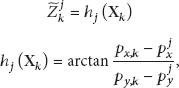
In order to better comprehend the tracking system, Figure 1 shows the measurement model of this system. At a given snapshot k, each active node can give a bearing with the DOA estimation for the target. Assume that the node measurement error obeys an additive white Gaussian noise model. Thus, for the active node j, the measurement $Z_k^j$ at the snapshot k is given by

$$\begin{array}{cc}& Z_k^j={\tilde{Z}}_k^j+{\omega }_k^j,\end{array}$$

(1)

where ${\tilde{Z}}_k^j$ denotes the true DOA for the node j and ${\omega }_k^j$ is a zero-mean white Gaussian noise with standard deviation ${\sigma }_j$ .

Figure 1

The measurement model of the tracking system.

According to the geometric relationship between the node location and the target position, ${\tilde{Z}}_k^j$ can be described by the following equations:

$$\begin{array}{cc}& {\tilde{Z}}_k^j=h_j\left({\mathbf{X}}_k\right)\\ h_j\left({\mathbf{X}}_k\right)=\arctan \frac{p_{x,k}-p_x^j}{p_{y,k}-p_y^j},\end{array}$$

(2)

where ${\mathbf{X}}_k$ is the target state containing the position and the velocity of the target, $h_j({\mathbf{X}}_k)$ represents the nonlinear function related to ${\mathbf{X}}_k$ , which is the arc tangent function denoted by arctan, and $[p_x^j,p_y^j]$ is the location of the node j in Cartesian coordinates.

2.2. Decentralized Extended Kalman Filter

After the active nodes have estimated the DOA of the target, the tracking system fuses all measurements of the active nodes to utilize the extended Kalman filter (EKF) for tracking. The EKF can be viewed as the nonlinear counterpart of the classical Kalman filter [28]. Because the decentralized system is considered, this paper uses the decentralized extended Kalman filter (DEKF) to complete the trace process.

The target state is denoted by ${\mathbf{X}}_k=[p_{x,k},p_{y,k},v_{x,k},v_{y,k}{]}^T$ , where $[p_{x,k},p_{y,k}{]}^T$ represent the x-axis and y-axis position components and $[v_{x,k},v_{y,k}{]}^T$ represent the x-axis and y-axis velocity components at the snapshot k. Then the state transition can be expressed as

$$\begin{array}{cc}& {\mathbf{X}}_k=f\left({\mathbf{X}}_{k-\mathrm{1}},k\right)+{\mathbf{B}}_k{\mathbf{W}}_k,\end{array}$$

(3)

where f is a state transition function which is subject to the target motion model, ${\mathbf{B}}_k$ represents the process noise distribution, and ${\mathbf{W}}_k$ is the process noise matrix which follows a zero-mean Gaussian distribution with covariance matrix ${\mathbf{Q}}_k$ .

Assume that there are M nodes participating in tracking at the snapshot k; then the measurements of all M nodes are denoted by ${\mathbf{Z}}_k=[Z_k^{\mathrm{1}},Z_k^{\mathrm{2}},\dots ,Z_k^j,\dots ,Z_k^M{]}^T$ , and hence ${\mathbf{Z}}_k$ can be written as

$$\begin{array}{cc}& {\mathbf{Z}}_k=h\left({\mathbf{X}}_k\right)+{\mathbf{V}}_k\\ h\left({\mathbf{X}}_k\right)={\left[\begin{array}{cccc}{h}_{\mathrm{1}}\left({\mathbf{X}}_k\right)& h_{\mathrm{2}}\left({\mathbf{X}}_k\right)& \cdots & h_M\left({\mathbf{X}}_k\right)\end{array}\right]}^T,\end{array}$$

(4)

where ${\mathbf{V}}_k=[{\omega }_k^{\mathrm{1}},{\omega }_k^{\mathrm{2}},\dots ,{\omega }_k^M{]}^T$ is the measurement noise matrix.

Like the Kalman filter, the DEKF also has two steps: the prediction step and the update step. The DEKF is carried out by the following equations.

(a)  The prediction step:

$$\begin{array}{cc}& {\mathbf{X}}_{k+\mathrm{1}\mid k}={\mathbf{F}}_k{\mathbf{X}}_k\\ {\mathbf{P}}_{k+\mathrm{1}\mid k}={\mathbf{F}}_k{\mathbf{P}}_{k\mid k}{\mathbf{F}}_k^T+{\mathbf{B}}_k{\mathbf{Q}}_k{\mathbf{B}}_k^T,\end{array}$$

(5)

where F and P, respectively, are the state transition matrix and the state covariance matrix about X. This step can be implemented for the prediction of X and P.

(b)  The update step:

$$\begin{array}{cc}& {\nabla }_j=\frac{\mathrm{1}}{r_j}{\left(-{\sin \varphi }_j,\cos {\varphi }_j,\mathrm{0,0}\right)}^T\end{array}$$

(6)

$$\begin{array}{cc}& {\mathbf{Y}}_{k+\mathrm{1}}^j=\frac{\mathrm{1}}{{\sigma }_j^{\mathrm{2}}}{\nabla }_j{\nabla }_j^T\end{array}$$

(7)

$$\begin{array}{cc}& y_{k+\mathrm{1}}^j=\frac{\mathrm{1}}{{\sigma }_j^{\mathrm{2}}}{\nabla }_j\left[Z_{k+\mathrm{1}}^j-h_j\left({\mathbf{X}}_{k+\mathrm{1}\mid k}\right)+{\nabla }_j^T{\mathbf{X}}_{k+\mathrm{1}\mid k}\right]\end{array}$$

(8)

$$\begin{array}{cc}& {{\mathbf{P}}_{k+\mathrm{1}\mid k+\mathrm{1}}}^{-\mathrm{1}}={{\mathbf{P}}_{k+\mathrm{1}\mid k}}^{-\mathrm{1}}+\sum _{j=\mathrm{1},\dots ,M}{\mathbf{Y}}_{k+\mathrm{1}}^j\end{array}$$

(9)

$$\begin{array}{cc}& {\mathbf{X}}_{k+\mathrm{1}\mid k+\mathrm{1}}={\mathbf{P}}_{k+\mathrm{1}\mid k+\mathrm{1}}\left({{\mathbf{P}}_{k+\mathrm{1}\mid k}}^{-\mathrm{1}}{\mathbf{X}}_{k+\mathrm{1}\mid k}+\sum _{j=\mathrm{1},\dots ,M}{y}_{k+\mathrm{1}}^j\right),\end{array}$$

(10)

where ${\nabla }_j$ is the gradient of $h_j(·)$ about ${\mathbf{X}}_{k+\mathrm{1}\mid k}$ and $[r_j,{\varphi }_j]$ is the polar representation of the node j location $[p_x^j,p_y^j]$ relative to the predicted target position $[p_{x,k+\mathrm{1}\mid k},p_{y,k+\mathrm{1}\mid k}]$ . In the update step, all active nodes share their measurements and obtain the updated target state and state covariance matrix by (6)–(10).

2.3. Foundation for Node Selection

The goal of NSP is to find out the best set of active nodes from all nodes in the WSN to track the target. In order to ensure the tracking accuracy, the information utility is usually considered to be a measure of the expected mean square position error. That is, if NSP select the active nodes set which has the largest information utility, then target tracking will get the least expected mean square position error.

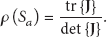
For example, the information utility of the active nodes set $S_a$ can be defined as the reciprocal of the posterior position error $\rho (S_a)$ , and thus it can be written as

$$\begin{array}{cc}& U\left(S_a\right)=\frac{\mathrm{1}}{\rho \left(S_a\right)}.\end{array}$$

(11)

According to the updated state covariance matrix in the DEKF, $\rho (S_a)$ can be given by

$$\begin{array}{cc}& \rho \left(S_a\right)={\mathbf{P}}_{k+\mathrm{1}\mid k+\mathrm{1}}\left(\mathrm{1,1}\right)+{\mathbf{P}}_{k+\mathrm{1}\mid k+\mathrm{1}}\left(\mathrm{2,2}\right),\end{array}$$

(12)

where $\mathbf{A}(a,b)$ is the $a_{\text{th}}$ row and the $b_{\text{th}}$ column element of the matrix A, and then ${\mathbf{P}}_{k+\mathrm{1}\mid k+\mathrm{1}}(\mathrm{1,1})$ and ${\mathbf{P}}_{k+\mathrm{1}\mid k+\mathrm{1}}(\mathrm{2,2})$ represent the position components of ${\mathbf{P}}_{k+\mathrm{1}\mid k+\mathrm{1}}$ which can be derived from (9). For simplicity, the inverse matrix of ${\mathbf{P}}_{k+\mathrm{1}\mid k+\mathrm{1}}$ ,   ${{\mathbf{P}}_{k+\mathrm{1}\mid k+\mathrm{1}}}^{-\mathrm{1}}$ , is denoted by ${\mathbf{J}}_f$ . Then (9) can be rewritten as

$$\begin{array}{cc}& {\mathbf{J}}_f={\mathbf{J}}_p+\left[\begin{array}{cc}\mathbf{J}& \mathbf{0}\\ \mathbf{0}& \mathbf{0}\end{array}\right]\\ {\mathbf{J}}_p={{\mathbf{P}}_{k+\mathrm{1}\mid k}}^{-\mathrm{1}}\\ \mathbf{J}=\sum _{j\in S_a}\frac{\mathrm{1}}{{\sigma }_j^{\mathrm{2}}{r}_j^{\mathrm{2}}}\left[\begin{array}{cc}{\sin }^2{\varphi }_j& -\sin {\varphi }_j{\cos \varphi }_j\\ -\sin {\varphi }_j{\cos \varphi }_j& {\cos }^{\mathrm{2}}{\varphi }_j\end{array}\right].\end{array}$$

(13)

Therefore, $\rho (S_a)$ can be obtained as follows

$$\begin{array}{l}\rho \left(S_a\right)=\left(\mathrm{tr}\left\{{\tilde{\mathbf{J}}}_p\right\}+\mathrm{tr}\left\{\mathbf{J}\right\}\right)\\ \hspace{1em}\times (\phantom{\left({\left[{\tilde{\mathbf{J}}}_p\right]}_{\mathrm{1,1}}\frac{\mathrm{co}{\text{s}}^{\mathrm{2}}{\varphi }_j}{{\sigma }_j^{\mathrm{2}}{r}_j^{\mathrm{2}}}+{\left[{\tilde{\mathbf{J}}}_p\right]}_{\mathrm{2,2}}\frac{{\sin }^2{\varphi }_j}{{\sigma }_j^{\mathrm{2}}{r}_j^{\mathrm{2}}}+\mathrm{2}{\left[{\tilde{\mathbf{J}}}_p\right]}_{\mathrm{1,2}}\frac{\sin {\varphi }_j\cos {\varphi }_j}{{\sigma }_j^{\mathrm{2}}{r}_j^{\mathrm{2}}}\right)\sum _{j\in S_a}^{}({\left[{\tilde{\mathbf{J}}}_p\right]}_{\mathrm{1,1}}\frac{\mathrm{co}{\text{s}}^{\mathrm{2}}{\varphi }_j}{{\sigma }_j^{\mathrm{2}}{r}_j^{\mathrm{2}}}+{\left[{\tilde{\mathbf{J}}}_p\right]}_{\mathrm{2,2}}\frac{{\sin }^2{\varphi }_j}{{\sigma }_j^{\mathrm{2}}{r}_j^{\mathrm{2}}}}\det \left\{\mathbf{J}\right\}+\det \left\{{\tilde{\mathbf{J}}}_p\right\}\\ \hspace{1em}\hspace{1em}\hspace{1em}+\sum _{j\in S_a}^{}({\left[{\tilde{\mathbf{J}}}_p\right]}_{\mathrm{1,1}}\frac{{\cos }^{\mathrm{2}}{\varphi }_j}{{\sigma }_j^{\mathrm{2}}{r}_j^{\mathrm{2}}}+{\left[{\tilde{\mathbf{J}}}_p\right]}_{\mathrm{2,2}}\frac{{\sin }^2{\varphi }_j}{{\sigma }_j^{\mathrm{2}}{r}_j^{\mathrm{2}}}\\ \hspace{1em}\hspace{1em}\hspace{1em}\hspace{1em}\hspace{1em}\hspace{1em}\hspace{1em}{+\mathrm{2}{\left[{\tilde{\mathbf{J}}}_p\right]}_{\mathrm{1,2}}\frac{\sin {\varphi }_j\cos {\varphi }_j}{{\sigma }_j^{\mathrm{2}}{r}_j^{\mathrm{2}}}))}^{-1}\end{array}$$

(14)

$$\begin{array}{l}{\tilde{\mathbf{J}}}_p={\left[{\mathbf{J}}_p\right]}_{\mathrm{1}\hspace{0.17em}:\hspace{0.17em}\mathrm{2,1}\hspace{0.17em}:\hspace{0.17em}\mathrm{2}}-{\left[{\mathbf{J}}_p\right]}_{\mathrm{1}\hspace{0.17em}:\hspace{0.17em}\mathrm{2,3}\hspace{0.17em}:\hspace{0.17em}\mathrm{4}}{\left({\left[{\mathbf{J}}_p\right]}_{\mathrm{3}:\mathrm{4,3}:\mathrm{4}}\right)}^{-\mathrm{1}}{\left[{\mathbf{J}}_p\right]}_{\mathrm{3}\hspace{0.17em}:\hspace{0.17em}\mathrm{4,1}\hspace{0.17em}:\hspace{0.17em}\mathrm{2}},\end{array}$$

(15)

where $[{\mathbf{J}}_p{]}_{a\hspace{0.17em}:\hspace{0.17em}b,c\hspace{0.17em}:\hspace{0.17em}d}$ is the submatrix of ${\mathbf{J}}_p$ which consists of rows a through b and columns c through d. The detailed derivation process can be referred to [6].

3. Node Selection for Tracking

The aim of node selection is to select an active nodes subset $S_a$ from the candidate nodes set $S_c$ that achieves better tracking accuracy with less cost of network at every snapshot. In the WSN, the nodes possess limited energy and lifetime, so balancing energy consumption strategy must be considered to prolong the lifecycle of network. This paper presents an energy-efficient node selection (EENS) algorithm, which is required to find the best set $S_a$ with up to M active nodes, where M is the constant number at each time snapshot. This section first introduces the system initialization process. Then, it describes the detailed steps of the EENS algorithm. Finally, it gives the summary of the ANS, GNS, and CLT algorithms.

3.1. System Initialization

Once a target appears in the monitoring area, the nodes deployed in this area will detect the target and give a bearing estimation of the target position. Then the tracking system should decide which nodes will participate in tracking. The objective of choosing nodes is minimizing the mean square localization error. Therefore, we use the GDOP metric to be a method of system initialization.

Assume that there are $N_s$ nodes in the WSN. We need to find the best nodes set $S_a$ of cardinality M from all $N_s$ nodes for tracking at the beginning. All nodes have already known the target position by the localization algorithm, which is not the content of this paper. Then, the posterior mean square position error by GDOP can be given by

$$\begin{array}{cc}& \rho \left(S_a\right)=\frac{\mathrm{tr}\left\{\mathbf{J}\right\}}{\det \left\{\mathbf{J}\right\}}.\end{array}$$

(16)

It can be seen that this equation is a simple expression of (14) where the prior information is ignored so that ${\tilde{\mathbf{J}}}_p=\mathrm{0}$ .

Therefore, the problem is to find the minimum of $\rho (S_a)$ , thereby determining which nodes compose the active set $S_a$ to observe the target at the next snapshot. Consider that all nodes communicate their locations with each other. Here, there are two methods to search the best nodes set for reference. One method is adopting an exhaustive strategy to try all combinations. However, this method has high computational complexity. For example, if the system decides to select M active nodes, then the number of computations is

$$\begin{array}{cc}& nc=\frac{N_s!}{M!\times \left(N_s-M\right)!}.\end{array}$$

(17)

The other method is “add one node at a time” (AOAT), where one node is chosen to be activated at a time. The details can be seen from [6]. It is minimizing the mean squared position error when adding a new node to $S_a$ . The system initialization process is shown in Figure 2.

Figure 2

The system initialization process.

3.2. EENS

After system initialization, the active nodes in $S_a$ have already been selected to track the target at the current snapshot k. At the same time, other nodes not belonging to $S_a$ go to sleep and keep a dormant mode. The system fuses the nodes measurements of $S_a$ so that ${\mathbf{X}}_{k\mid k}$ and ${\mathbf{P}}_{k\mid k}$ can be obtained by the updated steps of DEKF. Then the prediction of the target position is calculated for the following node selection. The EENS can be described from two perspectives, the active nodes and the idle nodes. More specifically, the first stage is that EENS selects a nodes subset $S_a^{-}$ with desired cardinality $N_d$ from $S_a$ to keep the active status, and the second stage is that it selects κ idle nodes to be activated at the snapshot $k+1$ .

3.2.1. The First Stage

The main task of this stage is to find the best active subset of $N_d$ nodes from $S_a$ that maximizes (11). Generally the nodes which are active at the current snapshot are also best for tracking at the next snapshot, because the target moving distance is so small that the network topology only changes a little. Therefore, the performance of node selection algorithms is affected by the parameter setting of $N_d$ . A detailed explanation of this problem is beyond the scope of this paper. This stage still utilizes the AOAT method to choose the best active nodes set labeled as $S_a^{-}$ while the unselected nodes are denoted as ${\tilde{S}}_a$ .

3.2.2. The Second Stage

The goal of EENS is to find out the active nodes set which can bring the largest information utility, save the cost of the network, and balance energy expenditure on each node. After the first stage, it is possible that an idle node can be better than a node in $S_a^{-}$ to join $S_a^{-}$ . Therefore, EENS needs to calculate the information utility of idle nodes $n{u}_i(S_a^{-})$ , the criterion of node selection ${\phi }_i(S_a^{-})$ and select the κ largest ones to be activated. EENS implements two steps to select the idle nodes to become active. The details are as follows.

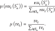
First, the active node j in $S_a^{-}$ computes its information utility by

$$\begin{array}{cc}& n{u}_j\left(S_a^{-}\right)=U\left(S_a^{-}\right)-U\left(S_a\setminus \left\{j\right\}\right).\end{array}$$

(18)

The maximum of the information utility of these nodes is denoted as the threshold Γ for other nodes to join $S_a^{-}$ . Then the active nodes in $S_a^{-}$ broadcast the target state prediction, their locations, and the threshold Γ.

Second, the idle nodes which receive information from all active nodes calculate their information utility $n{u}_i(S_a^{-})$ by

$$\begin{array}{cc}& n{u}_i\left(S_a^{-}\right)=U\left(S_a^{-}\cup \left\{i\right\}\right)-U\left(S_a^{-}\right).\end{array}$$

(19)

The information utility $n{u}_i$ is considered as an important metric for the idle node i to add to $S_a^{-}$ to become active. The greater the information utility $n{u}_i$ is, the more possible the node i is to be activated.

However, the distance of the target motion is usually so small that the current active nodes are probably also best at the next snapshot. Therefore, some nodes are always selected in $S_a^{-}$ , which makes these nodes consume energy faster. In order to balance energy expenditure on every node and extend the lifetime of the whole network, the residual energy of the node is introduced into the optimization of NSP. The criterion of NSP can be described as a mixture of information utility and the residual energy. Then the criterion for the node i to join $S_a^{-}$ is given by

$$\begin{array}{cc}& {\phi }_i\left(S_a^{-}\right)=\alpha ·\mu \left(n{u}_i\left(S_a^{-}\right)\right)+\left(\mathrm{1}-\alpha \right)·\mu \left(\text{r}{\text{e}}_i\right),\end{array}$$

(20)

where $\text{r}{\text{e}}_i$ represents the residual energy of the node i, α is the relative weighting of the information utility and residual energy, and $\mu (·)$ is the normalization function. Normalization is designed to let the information utility and residual energy of each candidate node have the same level of effects on ${\phi }_i$ . Therefore, the function $\mu (·)$ is defined by

$$\begin{array}{cc}& \mu \left(n{u}_i\left(S_a^{-}\right)\right)=\frac{n{u}_i\left(S_a^{-}\right)}{{\sum }_{i\notin S_a}^{}n{u}_i\left(S_a^{-}\right)}\\ \mu \left(\text{r}{\text{e}}_i\right)=\frac{\text{r}{\text{e}}_i}{{\sum }_{i\notin S_a}\text{r}{\text{e}}_i}.\end{array}$$

(21)

The first term in ${\phi }_i(S_a^{-})$ indicates the usefulness of the measurements of the node i. The usefulness means the improvement of the position estimation accuracy by the node i. The second term characterizes the effort of the residual energy on the node selection. The criterion fully considered the two factors with the value of α, and there is a bias toward the factor of a larger coefficient. In addition, the validity of this criterion can be proved by the two points: first, any one candidate node adding to $S_a^{-}$ can improve the information utility of the active nodes set, and the different nodes lead to different degree of the improvement, so the tracking performance can be ensured by the nodes in $S_a^{-}$ ; second, the introduction of the energy factor just make the node selection have a deflection but not affect the tracking correctness.

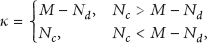
According to the quantity requirements for the nodes participants, we choose the nodes whose selected criterion ${\phi }_i(S_a^{-})$ are the κ largest ones, and thus the objective function can be defined as

$$\begin{array}{cc}& i=\arg \hspace{0.17em}\underset{i\notin S_a}{\text{large}}\left\{{\phi }_i\left(S_a^{-}\right),\kappa \right\}.\end{array}$$

(22)

In addition, the number of active nodes $N_a$ is a function of the parameters $N_d$ and κ at every snapshot. Because of the assumption that the active nodes number is up to M as mentioned above, the parameter κ can be obtained from

$$\begin{array}{cc}& \kappa =\{\begin{array}{cc}M-N_d,\hfill & N_c>M-N_d\hfill \\ N_c,\hfill & N_c<M-N_d,\hfill \end{array}\end{array}$$

(23)

where $N_c$ is the nodes number of the candidate set $S_c$ . In other words, $\kappa =\min \{N_c,M-N_d\}$ . Then, the active nodes number can be computed by

$$\begin{array}{cc}& N_a=N_d+\kappa .\end{array}$$

(24)

Now the set $S_a^{-}$ is relabeled as $S_a^{+}$ , which is the active nodes set at the next snapshot. Figure 3 shows the process of the EENS in a snapshot interval for node selection.

Figure 3

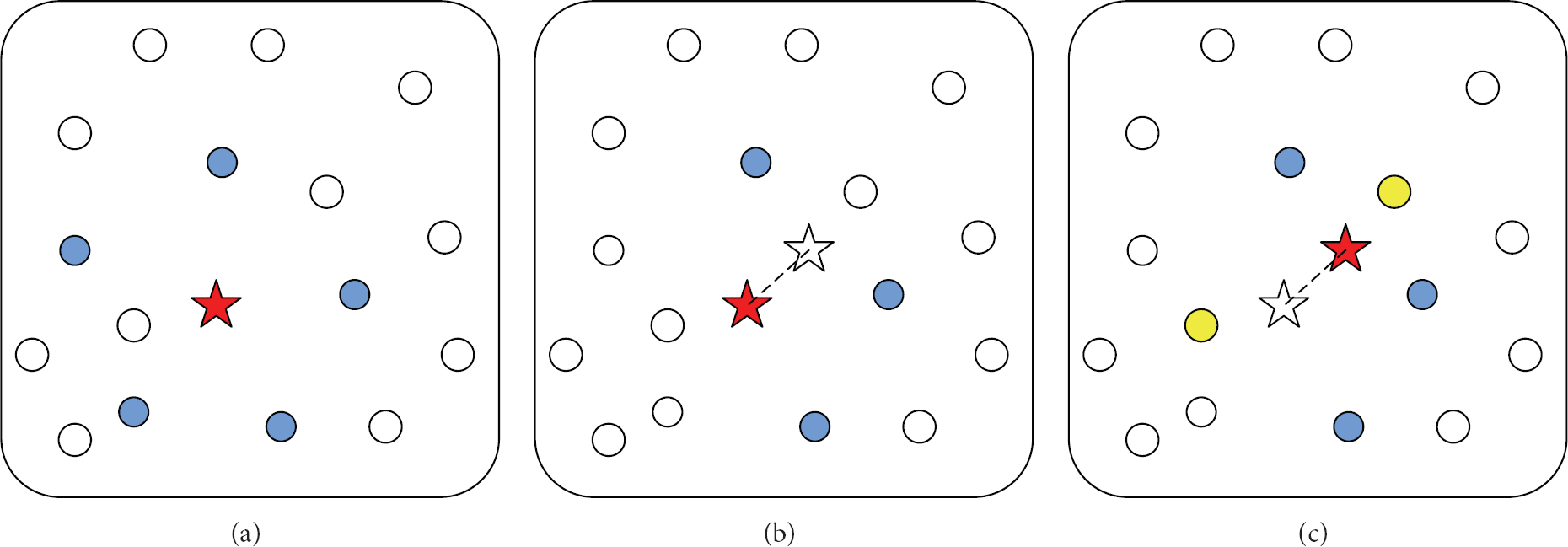
The process of the EENS in a snapshot interval. (a) The active nodes set $S_a$ denoted in solid circle at the current snapshot. (b) According to the predicted target position, EENS selects the active nodes set $S_a^{-}$ from $S_a$ . (c) EENS selects idle nodes denoted in solid yellow circle to join $S_a^{-}$ finally labeled $S_a^{+}$ .

Furthermore, the utility $n{u}_i$ is bounded above by a function of the distance between the target and the idle node i, which can be computed by

$$\begin{array}{cc}& n{u}_i\left(S_a^{-}\right)<\frac{\mathrm{1}}{{\sigma }_i^{\mathrm{2}}{r}_i^{\mathrm{2}}}.\end{array}$$

(25)

The proof can be seen in the appendix.

The upper bound of the information utility brought by an idle node can help to eliminate the nodes which are unable to be better than the nodes in $S_a^{-}$ and determine the candidate nodes set $S_c$ . According to this upper bound, the distance between the idle node i and the target should be

$$\begin{array}{cc}& r_i<r_{\Gamma }=\frac{\mathrm{1}}{{\sigma }_{\min }\sqrt{\Gamma }}.\end{array}$$

(26)

The nodes which can satisfy (26) are labeled as a candidate set $S_c$ .

The broadcast range of an active node needs to be set high enough to cover other active nodes in $S_a^{-}$ and the candidate idle nodes to join $S_a^{-}$ . Therefore, the broadcast range for the node $j\in S_a^{-}$ is

$$\begin{array}{cc}& d_j=r_j+r_c\\ r_c=\underset{}{\max }\left\{r_{\Gamma },\underset{j\in S_a^{-}}{\max }\hspace{0.17em}{r}_j\right\},\end{array}$$

(27)

where $r_c$ represents the critical range to the target to cover all active nodes and candidate nodes. In fact, only the nodes which fall in the communication range of the active nodes from the previous snapshot can be chosen to add to the next active nodes set. These available nodes form the candidate set $S_{\text{c}}$ .

3.3. ANS and GNS

The ANS algorithm uses different criteria to select idle nodes to join $S_a^{-}$ . As our presented algorithm, ANS also first choose $N_d$ nodes from $S_a$ to keep active mode by minimizing $\rho (S_a^{-})$ , but it defines the differential utility of an active node j in $S_a^{-}$ as

$$\begin{array}{cc}& \text{du}\left(j\right)=U\left(S_a^{-}\right)-U\left(S_a^{-}\setminus \left\{j\right\}\right)\end{array}$$

(28)

and the differential utility of an inactive node i as

$$\begin{array}{cc}& \text{du}\left(i\right)=\underset{j\in S_a^{-}}{\max }\left[U\left(S_a^{-}\setminus \left\{j\right\}\cup \left\{i\right\}\right)-U\left(S_a^{-}\setminus \left\{j\right\}\right)\right].\end{array}$$

(29)

Then these nodes in $S_a^{-}$ set a threshold τ for an inactive node to join the active set as the γth ( $\mathrm{1}\le \gamma \le N_d$ ) largest differential utility $\text{du}(j)$ , $j\in S_a^{-}$ . Active nodes broadcast the threshold, predicted target state and their location. Once the inactive nodes receive the data from the active set, they calculate their differential utility by (29). If the differential utility exceeds the threshold, then the node joins the active set. The ANS algorithm does not consider the energy factor in node selection.

Unlike ANS, although GNS incorporates the search stage of ANS, it uses all nodes within range of the $S_a$ active nodes to implement searching. In other words, GNS does not need to implement the steps of selecting the candidate nodes set and $N_a=N_d$ .

3.4. CLT

All nodes in the WSN know each node location after system initialization, so the active nodes can select idle nodes to become active at the next snapshot by the information of their close nodes. The CLT method simply selects the $N_a$ nodes with the smallest virtual range to the target. The virtual range is defined as

$$\begin{array}{cc}& \text{Vr}\left(i\right)={\sigma }_i{r}_i.\end{array}$$

(30)

Then this method sorts the virtual range so that it can choose the nodes. This method is computationally simple. However, its tracking accuracy is possible to be reduced due to the ignorance of the angular diversity of nodes.

4. Simulation

In order to demonstrate the effectiveness of the proposed method for node selection, we apply it to the WSN for bearings-only target tracking and compare it with CLT, GNS, and ANS in terms of the complexity, the execution time, the root mean square error (RMSE) of the target position estimation, energy consumption, and residual energy statistics on individual nodes.

Consider a scene that 50 nodes are uniformly deployed over a monitoring area of 1000 * 1000 m². The target occurs at $[-400,-400]$ and moves through the monitoring area with a constant velocity (CV) model. Figure 4 has shown the target trajectory with initial velocity of 20 m/s and nodes deployment in one trial. To illustrate the performance of different methods, 1000 Monte Carlo trials are generated for CLT, GNS, ANS, and EENS, respectively. The measurement noise of each node is a zero-mean Gaussian white noise with standard deviation ${\mathrm{5}}^{°}$ . For simplicity, we only consider the situation without prior information ( ${\tilde{\mathbf{J}}}_p=\mathrm{0}$ ). Here, the relative weighting parameter α of EENS is considered as 1 to testify the effectiveness of our proposed method. The effect of α on the node selection will be evaluated later.

Figure 4

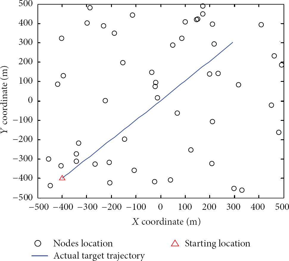
The target trajectory and nodes deployment.

Table 1 gives the computational complexity and the execution time of CLT, GNS, ANS, and EENS. The initial node selection at the beginning of target tracking uses the same method, as the system initialization in Section 3.1. Therefore, the comparison of the computational complexity focuses on the node selection at one time step. In other words, the total computations of node selection are calculated from the current snapshot to the next snapshot. The execution time is the average tracking time of 1000 Monte Carlo trials. The parameter setting is $N_d=\mathrm{2}$ and $M=\mathrm{5}$ . As can be seen from Table 1, GNS has the highest complexity, CLT has the simplest computations, and ANS and EENS have a satisfactory performance on the computational complexity and execution time.

Table 1

The computational complexity and the execution time of CLT, GNS, ANS, and EENS.

Methods	Total computations	Execution time/s
CLT	$N_a\times N_s$	0.031
GNS	$\frac{N_s\times (N_s-\mathrm{1})}{\mathrm{2}}+{\displaystyle \sum }_{m=\mathrm{2}}^{N_a-\mathrm{1}}(N_s-m)$	0.398
ANS	$\frac{N_a\times (N_a-\mathrm{1})}{\mathrm{2}}+{\displaystyle \sum }_{m=\mathrm{2}}^{N_d-\mathrm{1}}(N_a-m)+N_{c\_\text{ANS}}$	0.058
EENS	$\frac{N_a\times (N_a-\mathrm{1})}{\mathrm{2}}+{\displaystyle \sum }_{m=\mathrm{2}}^{N_d-\mathrm{1}}(N_a-m)+N_{c\_\text{EENS}}$	0.048

Figure 5 has shown the tracking performance comparison of four different node selection methods versus the average number of active nodes per snapshot. The average RMSE for Monte Carlo simulations can be seen from different symbols. The RMSE of CLT is far larger than the other three methods and EENS performs better than other methods overall. In addition, EENS can use less active nodes but achieve almost the same tracking accuracy or better than the other methods.

Figure 5

Comparison of tracking accuracy against the average number of active nodes.

The energy consumption results are compared in Figures 6–9. In this simulation, we refer to the communication model for WSNs in [29]. The energy to implement operations is far smaller than the energy to transmit data, so the simulation ignores the energy for calculations. Assume that the energy to transmit l bits of data a distance of d meters is

$$\begin{array}{cc}& E_t=l{\epsilon }_{\text{elec}}+l{\epsilon }_{\text{amp}}{d}^{\mathrm{4}}\end{array}$$

(31)

and the energy to receive the data is

$$\begin{array}{cc}& E_r=l{\epsilon }_{\text{elec}},\end{array}$$

(32)

where ${\epsilon }_{\text{elec}}$ represents the energy per bit to run the electronics, and ${\epsilon }_{\text{amp}}$ is the energy per bit to run the power amplifier. Given ${\epsilon }_{\text{elec}}=\mathrm{0.5}\times \mathrm{1}{\mathrm{0}}^{-\mathrm{7}}\hspace{0.17em}\text{J}/\text{bit}$ , ${\epsilon }_{\text{amp}}=\mathrm{1.3}\times \mathrm{1}{\mathrm{0}}^{-\mathrm{14}}\hspace{0.17em}\text{J}/\text{bit}/{\text{m}}^{\mathrm{4}}$ and $l=\mathrm{500}\hspace{0.17em}\hspace{0.17em}\text{bits}$ . Figure 6 shows the average energy consumption of the entire network per tracking process against the average number of active nodes. The comparison result of CLT, GNS, ANS, and EENS is shown in Figure 6(a). Consistent with the practical experience, the network costs more energy as the active nodes number increases. It can be seen that CLT consumes the maximum amount of energy and GNS is the second. This is because when the network uses CLT and GNS for node selection, the nodes need to communicate each other to get the knowledge of all nodes with more power consumption. However, the nodes in ANS and EENS only use their local information, so ANS and EENS can save much energy and do not be affected once the network topology changes. In order to see the difference between ANS and EENS more clearly, Figure 6(b) shows the enlarged figure of the rectangular portion with the green dashed line in Figure 6(a). From Figure 6(b) we can see that EENS uses less energy consumption than ANS.

Figure 6

The average energy consumption of the entire network per tracking process against the average number of active nodes. (a) The comparison result of CLT, GNS, ANS, and EENS. (b) The enlarged figure of the rectangular portion with green dashed line in (a).

Figure 7

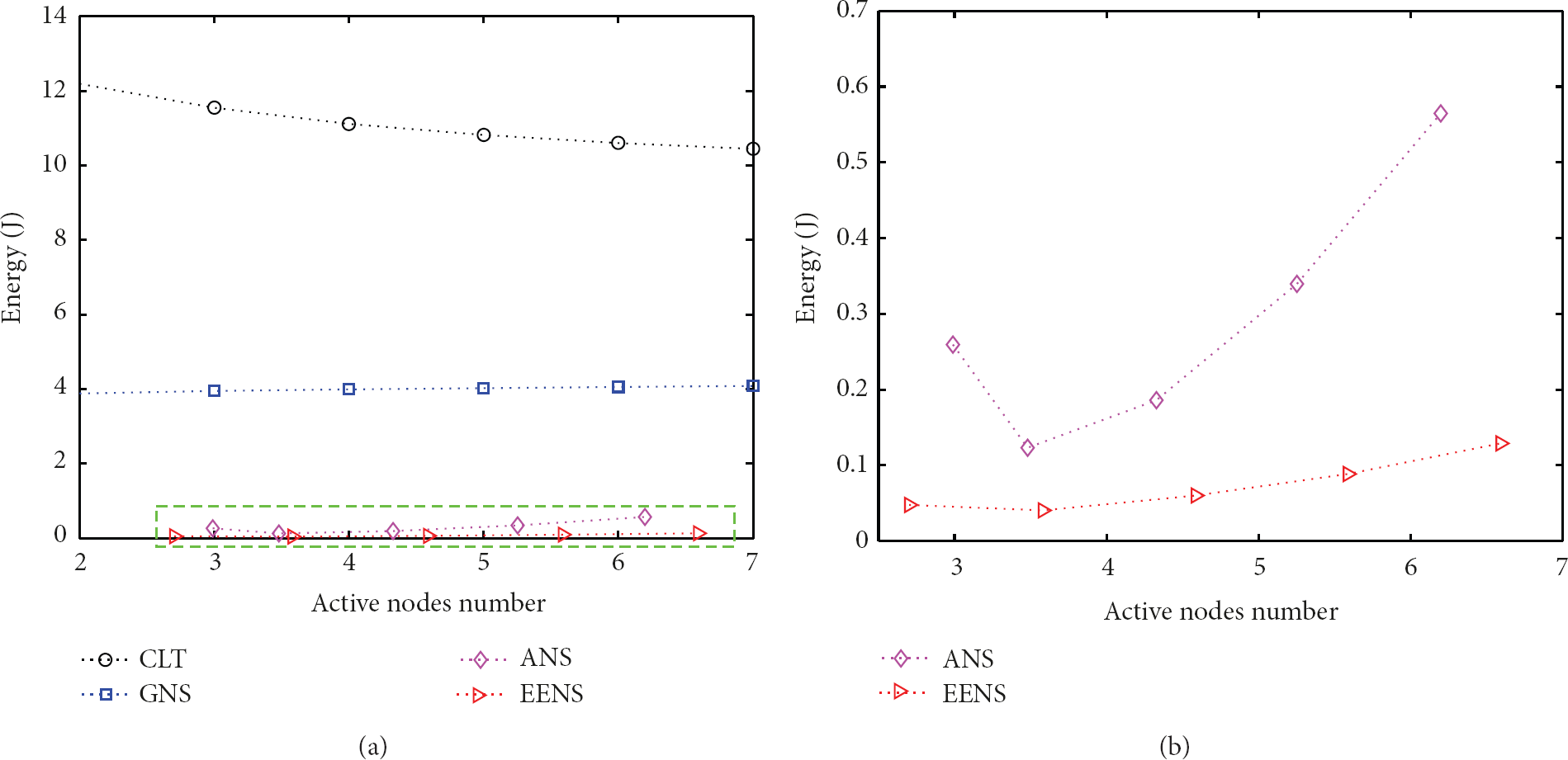
The average energy consumption of the entire network per tracking process against RMSE. (a) The comparison result of CLT, GNS, ANS, and EENS. (b) The enlarged figure of the rectangular portion with green dashed line in (a).

Figure 8

The average energy consumption per node against the average number of active nodes. (a) The comparison result of CLT, GNS, ANS, and EENS. (b) The enlarged figure of the rectangular portion with green dashed line in (a).

Figure 9

The average energy consumption per node against RMSE. (a) The comparison result of CLT, GNS, ANS, and EENS. (b) The enlarged figure of the rectangular portion with green dashed line in (a).

Figure 7 gives out the average energy consumption of the entire network per tracking process against RMSE. Similarly to Figure 6, Figure 7(a) shows the comparison result of the four different algorithms and Figure 7(b) shows the enlarged figure of the rectangular portion with the green dashed line in Figure 7(a). From Figure 7(a) it can be seen that ANS and EENS can expend substantially less energy with meeting the requirements of tracking accuracy. To better see the performance comparison of ANS and EENS, Figure 7(b) shows that EENS has a significant decrease of energy consumption.

Note here that there is each inflection point in Figures 6(b) and 7(b). Its presence does not comply with the common apperception rule. The reason is the refreshing phenomenon which occurs in ANS when an active set of two nodes becomes collinear with the target [9], which leads to abundant nodes to join target tracking. For example, when the active nodes number is about 3 (the parameter $N_d$ of ANS is general to be 2), ANS easily makes a large amount of the nodes to be activated and consumes more energy, so the left-most point of ANS in Figure 6(b) is higher than the next point in the y axis. In the same way, the right-most point of ANS in Figure 7(b) can be explained.

Figures 8 and 9 have shown the average energy consumption per node against the average number of active nodes and RMSE, respectively. The results of these two figures are in accord with Figures 6 and 7.

The above simulation results obviously show that the EENS method is effective and energy efficient. However, these simulations set the parameter $\alpha =\mathrm{1}$ in EENS. In order to verify the role of α in EENS, we simulate EENS with $\alpha =\mathrm{0.2}$ , $\alpha =\mathrm{0.5}$ , $\alpha =\mathrm{0.8}$ , and $\alpha =\mathrm{1}$ to compare the performance for 1000 Monte Carlo trials. Because of the relatively good performance of ANS compared to CLT and GNS, we use ANS as the reference to the different parameter settings of EENS. Table 2 gives out the performance comparison results with $N_d=\mathrm{2}$ and $M=\mathrm{5}$ . It shows that EENS with different α also have good tracking accuracy and energy efficiency. However, the performance of EENS with different α does not appear regular change as α gets larger. The impact of α makes the node selection bias towards the larger weight between the information utility and the residual energy of the node. It does not impact the tracking performance and energy consumption directly.

Table 2

The performance comparison of ANS and EENS with different parameter settings.

Methods	Active nodes number	RMSE (m)	Average energy consumption of network per tracking process (J)	Average energy consumption per node (J)
ANS	3.0412	3.2084	45.632	0.3001
EENS ( $\alpha =\mathrm{0.2}$ )	3.3989	2.8497	5.7986	0.0341
EENS ( $\alpha =\mathrm{0.5}$ )	3.3961	2.8626	5.8021	0.0342
EENS ( $\alpha =\mathrm{0.8}$ )	3.3963	2.8510	5.8094	0.0342
EENS ( $\alpha =\mathrm{1}$ )	3.3961	2.8560	5.7975	0.0341

Besides, the smaller the parameter α, the criterion of node selection as (20) is more considering the residual energy of the node than the information utility brought by the node, so EENS prefers to select the nodes which have more power, and then the energy consumption of the entire network is more even. This is consistent with the result of Figure 10. Figure 10 illustrates the residual energy statistics on individual nodes. It can be seen that the number of nodes which have less or more residual energy is smaller using $\alpha =\mathrm{0.2}$ than other values, as the residual energy is on the interval $[\mathrm{10,50}]$ or $[\mathrm{80,110}]$ . This shows that the energy expenditure on nodes is more even with $\alpha =\mathrm{0.2}$ , but in other parameters, some nodes consume more energy because they are selected many times even if their residual energy is little. Therefore, EENS is able to balance the energy expenditure for the WSN.

Figure 10

The residual energy statistics on individual nodes.

5. Conclusion

This paper proposed an energy-efficient node selection for bearings-only target tracking in WSNs. This method redefines the information utility of the idle node to join the active nodes set and introduces the factor of the residual energy into the objective function for node selection. It makes the criterion of choosing at most M nodes to participate in tracking. In the decentralized WSN, the proposed method only uses the local information of the node so it can save more energy and better accommodate to the change of networks. The incorporation of the factor of the residual energy makes the control of the entire network easier. According to the setting of the weighting parameter, the network can balance the energy consumption on nodes and extend the life of the network. Simulation results validated the good performance of the proposed method in terms of tracking RMSE, energy expenditure, and the residual energy statistics on individual nodes.