Application of Computational-Experimental Methods for Designing Optimized Semitrailer Axle Supports

Abstract

Computational and experimental methods were applied to the design and optimization of a semitrailer axle support subjected to fatigue loads. Numerical results based on the finite element method (FEM) were correlated with extensometric tests to assess the accuracy of the computational method. This paper is focused on the “minimum radius manoeuvre.” This situation represents the highly critical load case occurring in a semitrailer operation where the tractor vehicle pulls the semitrailer's kingpin at approximately 90° with respect to its longitudinal axis, and high stress and strain phenomena take place in the axle supports’ structure. Loads and boundary conditions that correspond to this load case were first adjusted by means of experimental tests and could be later applied to each semitrailer axle support in the numerical model. In this analysis, the stress-strain elastic-plastic curves of the base material, the welding, and the HAZ have been incorporated to the numerical models. Fatigue S-N curves combined with the maximum Von Mises equivalent stresses obtained in the computational analysis provided a maximum number of cycles that the semitrailer axle support could reach in case of the minimum radius manoeuvre being applied to the vehicle in a repeated manner. The initial design could then be optimized to improve its fatigue life.

1. Introduction

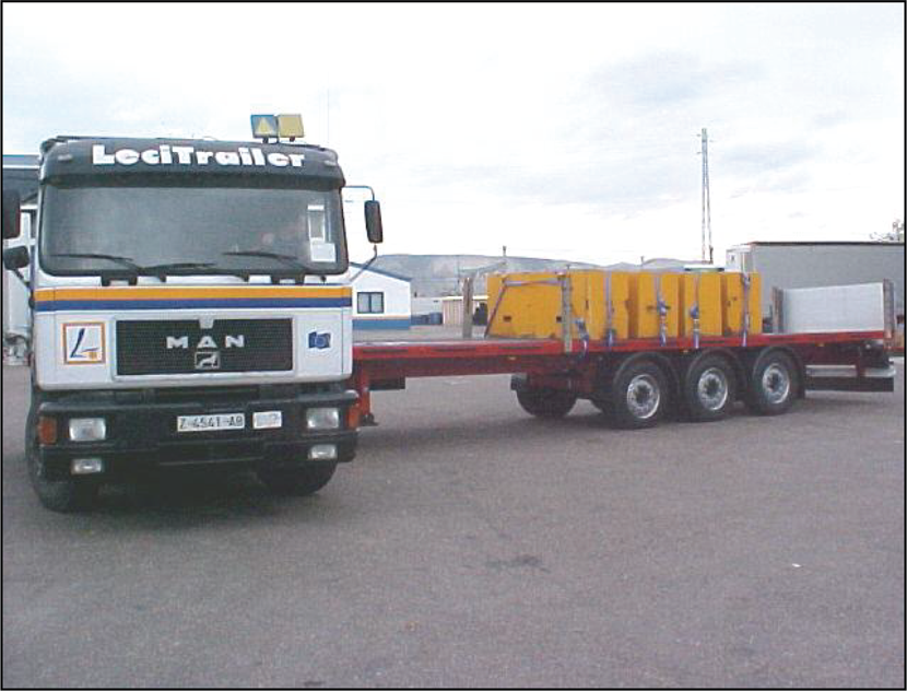
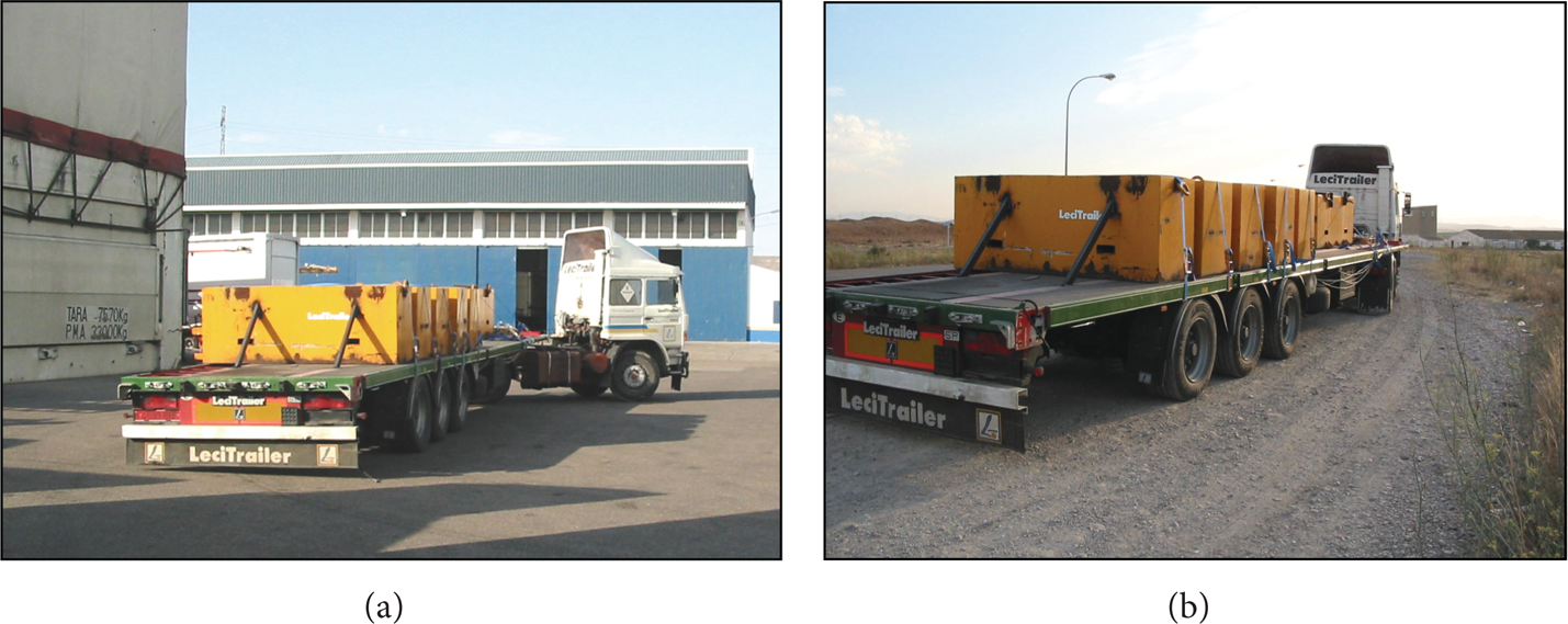
Competitiveness, weight reduction, fuel savings, and environmental and manufacturing factors are currently guiding semitrailer manufacturers to improve their new vehicle designs by means of modern computational tools. Therefore, new methodologies are needed to develop optimal structural solutions at lower costs and much less time than those necessary with the traditional trial and error methods [1–3]. This paper develops the process to obtain a new concept of semitrailer axle support, which can be applied to the current semitrailer market. In order to achieve this objective, a standard three-axle semitrailer structure was numerically and experimentally analyzed and several changes were identified from the results obtained in an initial analysis. A fatigue analysis of the structure was also carried out and the maximum number of cycles that the structure can reach until it breaks down was obtained for each steel component. Figure 1 shows a standard three-axle semitrailer as well as a detail of the configuration considered in the axle support structure analyzed. This vehicle basically consists of two I-shaped section longitudinal beams joined by welded transversal beams which are enclosed with front, rear, and side steel profiles making up a load-carrying platform. Each axle support structure comprises two additional crossbeams, two supports, and several reinforcements welded together as well as to the main longitudinal beams. The semitrailer analyzed is equipped with a pneumatic suspension system.

Figure 1:

(a) Three-axle semitrailer (LeciTrailer S.A.). (b) Axle support structure of the semitrailer.

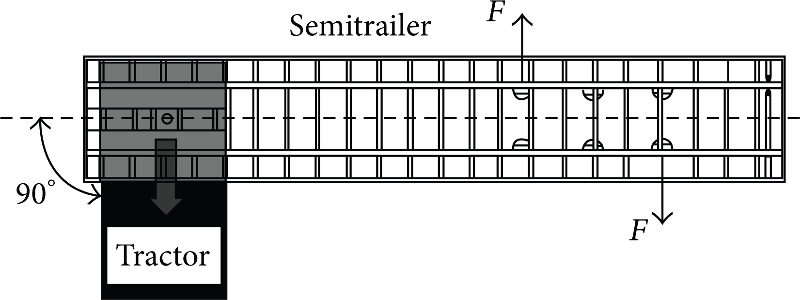
One of the most unfavourable load cases that can be applied to this structure occurs when the semitrailer is performing a “minimum radius manoeuvre,” situation at which the semitrailer is pulled at low speed by the driver's cab approximately in the shape of a 90-degree angle, as shown in Figure 2. Despite the fact that high forces and moments are involved in this manoeuvre, depending on the dimensions and the free space available in the loading-unloading facilities, this situation could be very usual. So when this manoeuvre is repeated in time during its normal operation, fatigue failure could be induced in some structural areas of the axle support [4]. Therefore, it is very important to quantify the loads that would appear in this critical manoeuvre to achieve an improved and more durable design of the axle support structure. This loads’ system was obtained by means of the combination of an extensometric test performed on a prototype of the semitrailer axle support and preliminary FE simulations.

Figure 2:

Tractor-semitrailer position considered in the “minimum radius manoeuvre.”

Once the load and boundary conditions were obtained, the mechanical behaviour of the axle support structure could be assessed by FE numerical analyses. First of all, a computational FE mesh model of the structure was created and different typologies of finite elements were used for achieving a high detail discretization of all components comprising one axle's support. Moreover, the welding effect on the material properties was also included in the model by means of mesh elements simulating not only the weld beads but also their surrounding heat affected zones. In order to validate the different finite element models used in the present study, extensometric tests were carried out so as to assess the strain values at several measuring points of the supports and to be able to contrast the theoretical values obtained in the numerical simulations with them.

As main contribution of the present study, it was possible to obtain a force-moment system able to reproduce and simulate with high accuracy the loads appearing in the minimum radius manoeuvre. This innovative methodology made it possible to propose, assess, and then introduce some changes on the initial design of the axle support structure so as to improve not only its mechanical performance but also its fatigue behaviour, increasing the maximum number of manoeuvre cycles that the axle support can hold up without failure.

2. Numerical Simulation Based on the FEM

2.1. General Considerations of the FE Modelization

All FE models developed in this study were preprocessed in PATRAN and then calculated and postprocessed with the software ABAQUS Standard. In particular, nonlinear static analyses were used in the simulations, taking into account the elastic-plastic behavior of metallic materials and choosing an appropriate typology of finite element for each structural component [5]. There are five aspects of a finite element that characterize its behavior: element family, degrees of freedom, number of nodes, formulation, and integration.

Degrees of freedom are those fundamental variables calculated during the analysis. In this case of static stress analysis, the considered degrees of freedom are translations and rotations. Although these variables are calculated at each node of the element, values in any other point of the element are obtained interpolating from their nodal values. The number of nodes used in an element usually determines its interpolation order: elements that have nodes only at their corners use linear interpolation for each direction and are often called first-order elements and elements with midsize nodes use quadratic interpolation instead and are called second-order elements. With respect to the element formulation, it refers to the mathematical theory used to define the element behaviour; for instance, in a shell element can be considered a “thin” or “thick” behaviour depending on the thickness modelled. The FE software uses numerical techniques to integrate various quantities over the volume of each element, thus allowing a complete generality and continuity of the material behaviour. Using Gaussian quadrature, the material response can be assessed at each integration point of every element. When using continuum elements, it must be chosen between full or reduced integration depending on the problem because this could have a significant effect on the accuracy of the element [6, 7].

2.2. FE Model of the Vehicle Structure (Mesh Considerations)

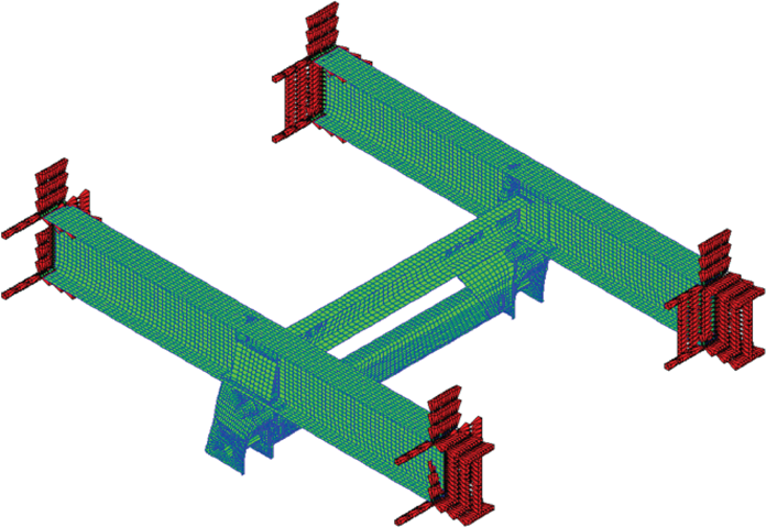
It has to be pointed out that only a portion of the semitrailer has been simulated in the numerical model, concretely the portion containing the complete axle support structure for one of its axles. This simplification was considered after defining the load case and the vehicle typology because, as can be observed in Figure 12, in a three-axle semitrailer the minimum radius manoeuvre load case would be equivalent to a force pair (generated by the tyre-ground friction) acting on the first and third axles of the vehicle while the central axle remains unloaded. Therefore, the developed model only corresponded to one of the loaded axles. The use of a simplified model instead of a complete vehicle model implied important cost reductions and savings in terms of computational time and modelization. All in all, the numerical model comprised 17.363 elements and 17.762 nodes. Figure 3 shows the whole finite element model of the axle support as well as each of its parts.

Figure 3:

(a) Finite element model of the axle support structure. (b) Modeled parts.

Due to the low thicknesses present in the axle support steel components (mainly made of laminated steel and bent steel plates), most of the elements used in the model were three-node (S3R) and four-node (S4R) planar shell elements with reduced integration. Three- and four-node planar rigid elements (R3D4 and R3D3) have also been used in the simulation of the small axle located inside and at the bottom of each support part. Therefore, these small axles presented the mechanical behaviour of an ideal rigid in the analyses, simulating an infinite stiffness at the same time that all displacements in each rigid configuration were constrained to one specific reference node. By this way, loads equivalent to those loads appearing in the analyzed manoeuvres could be applied to these reference points, which transmitted them to each axle support and then, from the supports, to the rest of the structure. Weld beads were instead modelled by means of C3D6 and C3D8R solid elements with six and eight nodes, respectively. Due to the weld beads’ geometry and location in the structure, these element types were considered the most appropriate to simulate the weld metal. Nevertheless, the use of solid elements in the simulation of the welded lap joints between planar parts located face to face made necessary the use of solid C3D6 and C3D8R elements in the modelization of the steel reinforcements that appear colored green in Figure 3. Figure 4 shows a mesh detail for two weld beads in the model. While the figure on the right simulates the joint between two parts modelled with shell elements, the figure on the left simulates the joint between solid and shell elements from different parts. Solid C3D6 elements were used in both cases for simulating the weld beads and, as can be seen, the solid elements’ faces shared equivalent nodes with the adjacent parts for achieving the assembly. Similarly, all assemblies in the model were simulated by means of equivalent nodes shared by different parts.

Figure 4:

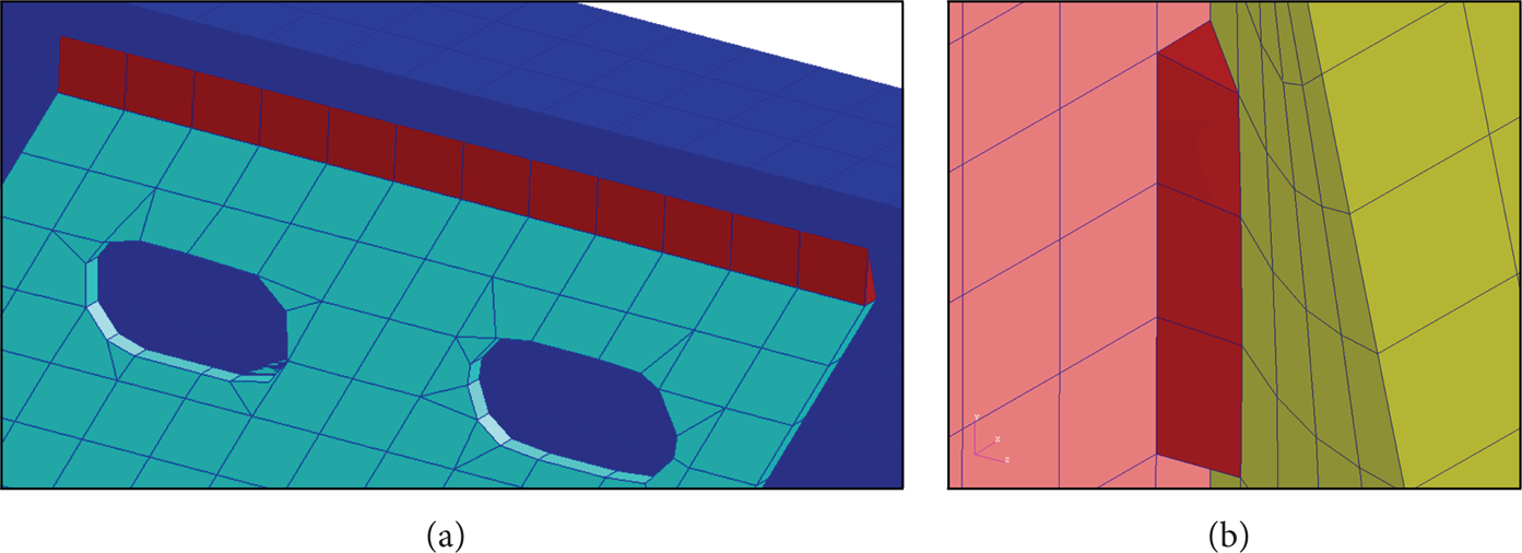
Weld bead models. (a) Solid-shell joint. (b) Shell-shell joint.

The element size chosen for the mesh model was approximately 20 mm (edge length). This value was considered appropriate to simulate the structure accurately without involving an excessive number of elements that would increase the time consumption during the calculations.

3. Modelization of the Materials’ Mechanical Properties

3.1. Elastic-Plastic Behaviour Curves

The initial analysis was performed using A-52 steel [8] for each one of the components comprising the axle support structure and the longitudinal beams. The steel mechanical behaviour was modelled with an isotropic elastic-plastic material model that corresponds to the Mises classic metal plasticity [5]. The steel strain-stress curves introduced in ABAQUS were approximated as bilinear curves taking into account the material's Young modulus, the yield strength, the tensile strength, the elongation at break, and Poisson's modulus (Figure 5).

Figure 5:

Strain-stress curve used to characterize the steel mechanical behaviour in ABAQUS.

With respect to the weld beads’ material and the adjacent HAZs resulting from the high temperature gradients present when the weld is made in the steel components, their mechanical properties were also simulated as isotropic elastic-plastic with the Mises classic metal model. Nevertheless, in this case, the material mechanical properties were obtained from Vickers hardness tests performed on welded specimens made of the same materials and welded with the same welding procedure specifications. Figure 6 shows the different areas defined in the mesh model not only for the weld beads but also for the HAZs, which simulate the different material regions obtained when different parts are welded together. A mesh detail of one of the welded joints located in the axle support is also shown in Figure 7.

Figure 6:

Mesh regions defined in the FE model for the assignment of material properties.

Figure 7:

Detailed view of a welded joint in the axle support structure.

Vickers hardness tests were carried out according to the UNE EN ISO 6507:1999 standard [9] on a five-millimeter-thick welded plate which was previously divided into three different areas: HAZ 1, HAZ 2, and HAZ 3, as shown in Figure 6. While HAZ 1 was located next to the weld metal, HAZ 3 was the furthest one. Apart from the HAZs, a different zone was also considered for the material under the weld metal. Since, from a macrographic analysis, a total HAZ width of approximately 9 mm was obtained, this value was incorporated to all welded joints of the mesh model: a width of 3 mm was considered for each HAZ stripe. Once the plate was cut and polished, two lines of material described as L1 and L2 were symmetrically swept along the thickness of the plate, each one containing fifteen indentation positions; Vickers hardness tests’ results are shown in Figure 8. Positions 7, 8, and 9 correspond to steel regions under the weld metal, positions 4 and 12 correspond to HAZ 3, positions 5 and 11 correspond to HAZ 2, and, finally, positions 6 and 10 correspond to HAZ 1.

Figure 8:

Vickers hardness values obtained.

Taking into account the existing relationship between strength and hardness over a wide range of strengths that is present in carbon and alloy steels with different pretreatments, the tensile strength at each zone could be obtained [10]. These equivalent tensile strength values are shown in Table 1. The medium values corresponding to each zone were calculated and are also pointed out in this table.

Table 1:

Equivalent tensile strength values according to Vickers hardness test results.

Indentation position	Metal zone	Test line 1		Test line 2		Average value of equivalent tensile strength (MPa)
		Vickers hardness(HV 10)	Equivalent tensile strength(MPa)	Vickers hardness(HV 10)	Equivalent tensile strength(MPa)
6 10	HAZ 1	248 256	805 876	236 240	804 815	825
5 11	HAZ 2	221 230	728 764	233 215	800 718	752
4 12	HAZ 3	225 230	744 764	215 191	718 632	714
7 8 9	Under weld zone	230 233 235	774 800 800	228 225 233	764 744 800	780

The rest of the values necessary to define the elastic-plastic behaviour of each zone with stress-strain curves were obtained by means of the following procedure.

• Young's modulus and the density of steel were considered for all the HAZs and under weld zones.

• The slope of the line defining the plastic behaviour at each zone was considered the same as the plastic slope present in the bilinear stress-strain curve of the original material.

• The area below the stress-strain curve corresponding to each zone was considered the same as the area present in the stress-strain curve of the original material. This area represents a measurement of the strain energy absorbed by the material when it is subjected to deformation.

By this way, the stress-strain curves of all zones could be defined as shown in Table 2, which collects all the parameters approximated by this procedure as well as the materials’ mechanical properties introduced in the FE model.

Table 2:

Mechanical properties of materials used in the FE model.

	St-52 steel	St-42 steel	Weld beads	Under weld zone	HAZ 1	HAZ 2	HAZ 3
Density (kg/m3)	7.800	7.800	7.800	7.800	7.800	7.800	7.800
Young's modulus (MPa)	210.000	210.000	210.000	210.000	210.000	210.000	210.000
Poisson's modulus	0,3	0,3	0,3	0,3	0,3	0,3	0,3
Yield strength (MPa)	410	260	410	718	767	688	647
Tensile strength (MPa)	510	420	560	780	825	752	715
Elongation at break (%)	20	20	26	16	15	17	18

3.2. Material Fatigue Behaviour Definition with S-N Curves

Fatigue failure was assessed by means of Wöhler S-N diagrams, which represented the stress-life curves for all the materials comprising the axle support structure. S-N diagrams show the nominal stress amplitude in a material (S) versus the cycles of failure (N); in this case, a semilog plot was used where stresses were covered in a linear scale and the cycles of failure in a logarithmic scale. Taking into account that steel presents a fatigue limit at which the curve stays horizontal, representing the stress value below which it can resist an infinite number of cycles [11], there exist procedures to generate the S-N diagrams from appropriate test data. A conventional steel S-N diagram is shown in Figure 9. It has to be pointed out that these curves are valid for cyclic stresses where loads are applied and removed in opposite directions. In this sense, it was considered that the minimum radius manoeuvre would be applied equally at both sides of the vehicle (i.e., at both turning directions), during the semitrailer's lifespan.

Figure 9:

Conventional steel S-N diagram.

Parting from the mechanical properties specified previously for each material and heat affected zone, several approximations and simplifications were necessary to define the materials’ S-N curves.

• The fatigue limit of each material was considered the 50% of its tensile strength [12, 13].

• The number of cycles corresponding to infinite life in steel was supposed to be between 10⁶ and 10⁷ cycles. In this case, it was fixed in 10⁷ cycles for all the materials.

• Tensile strength of each material was assigned a low number of load cycles until failure in the S-N diagram. The range of 1 ÷ 1000 cycles is generally defined as low cycle fatigue [11]; in this case, instead of 1000 cycles, a more conservative value of 100 cycles was fixed as the maximum N value for all considered materials at which tensile strength is reached.

Figure 10 shows how the simplified S-N curve was obtained, which was made up of three linear zones defined by the points a, b, c, and d. S_ut is the ultimate or tensile strength and S _e is the endurance or fatigue limit.

Figure 10:

S-N curve approximated for the fatigue analysis.

Finally, the resulting S-N curves estimated for the materials considered in the analyses are shown in Figure 11. The maximum values of equivalent stress obtained in the numerical analysis at each material and HAZ could by this way be applied to the corresponding S-N material curve in order to estimate the number of cycles of fatigue failure (N) for each axle support component.

Figure 11:

S-N curves approximated for the materials used in the analysis.

Figure 12:

Detail of semitrailer performing a minimum radius manoeuvre.

4. Load Case and Boundary Conditions

As stated before, one of the most critical load cases applied to the vehicle structure takes place when the semitrailer is performing a “minimum radius manoeuvre.” In this case, the tractor forms approximately a 90-degree angle with the semitrailer as it pulls from the kingpin. A detail of this maneuver is shown in Figure 12. When the tractor pulls the semitrailer, the loads system can be simplified as an equivalent system consisting in a couple of friction forces appearing in the tyre-ground contact of the first and third axles of the semitrailer, at the same time that the kingpin has the displacements constrained.

All the forces that act on each one of the wheels in the first and the third axles are transmitted to the axle supports through some different force-couple equivalent systems taking into account the overall size of the structure. In the case analyzed, the semitrailer was supposed to transport a load of 27 tons. While Figure 12 shows in a schematic way how the “minimum radius manoeuvre” is developed, Figure 13 shows the system of forces and moments (equivalent to the force couple system at Figure 12 on the right) that were created for simulating this load case.

Figure 13:

System of forces and moments considered in the “minimum radius manoeuvre” for the first axle.

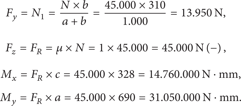
As can be observed in Figure 13, the ground reaction force N and the friction force F _R acting on the tyre (marked in red) were transformed into an equivalent system comprising forces F _y and F _z and moments M _x and M _y acting on the support (M _z = 0, due to the joint rotation) and the vertical force N₂ applied to the air spring. Since this study was focused on obtaining the tyre-ground forces that are transmitted through the axle support, it was not necessary to consider the diapress force N₂ and only the support forces and moments F _y , F _z , M _x , and M _y were taken into account in the analysis. As stated in the model description, these loads were applied to the reference points of the small axle located at the bottom of each support. As shown in Figure 13, these small axles are connected to the wheels’ axles by means of articulated steel arms that were not included in the model. Figure 14 shows the load application points in charge of transmitting the loads to the rest of the structure.

Figure 14:

Load application points in the FE mesh model.

An iterative procedure combining experimental and numerical results was developed in order to adjust this simplified loads’ system to the real situation as much as possible. In reality, the friction coefficient between the tyres and the ground is not known; moreover, M _x and M _y values depend on design, assembly, and rigidity parameters of the wheels and the suspension system's elements.

With respect to the boundary conditions, it was assumed that all nodes at both ends of the longitudinal beam stretches modelled were fully constrained (Figure 15). Since this model represented the first axle's support, these symmetric boundary conditions resulted from the hypothesis that, in the first place, this equivalent load case would correspond to having the kingpin constrained (end at −x-axis) and that, in the second place, inverse forces and moments would appear in the third axle's support of the semitrailer, which could be approximated with a constraint condition at the opposite end of each longitudinal beam stretch (end at +x-axis).

Figure 15:

Constrained nodes in the FE mesh model.

5. Estimation of Load Transmission Parameters for the Minimum Radius Manoeuvre Load Case

An experimental and numerical methodology was proposed to adjust the forces and moments applied to the numerical model as much as possible to the real performance of the axle's support when a minimum radius manoeuvre takes place. Therefore, it was necessary to define several parameters able to transform accurately the forces appearing in the tyre-ground contact into forces and moments applied directly to the supports (Figure 26).

5.1. FE Analyses with Loads Applied Independently

On the one hand, four different load cases were analyzed in ABAQUS, each one corresponding to the ideal application of loads F _y , F _z , M _x , and M _y independently to the FE model defined previously. The following considerations were taken into account in these numerical analyses.

• The friction force was calculated with a tyre-ground friction coefficient equal to 1.

• The ground reaction force N was defined for a transported freight of 27 tons and this situation was approximated as a vertical force equal to 90.000 N supported by each axle of the semitrailer (45.000 N at each support).

• Moments M _x and M _y were directly obtained from distances a, b, and c and the friction force F _R (Figure 13).

As a result of this, the following values were obtained:

$\begin{array}{c}{F}_y=N_{\mathrm{1}}=\frac{N\times b}{a+b}=\frac{\mathrm{45.000}\times \mathrm{310}}{\mathrm{1.000}}=\mathrm{13.950}\hspace{0.17em}\text{N},\\ F_z=F_R=\mu \times N=\mathrm{1}\times \mathrm{45.000}=\mathrm{45.000}\hspace{0.17em}\text{N}\left(-\right),\\ M_x=F_R\times c=\mathrm{45.000}\times \mathrm{328}=\mathrm{14.760.000}\hspace{0.17em}\text{N}·\text{mm},\\ M_y=F_R\times a=\mathrm{45.000}\times \mathrm{690}=\mathrm{31.050.000}\hspace{0.17em}\text{N}·\text{mm}.\end{array}$

(1)

In the postprocess phase of each analysis, the plane strain numerical values ∊ _x , ∊ _y , and γ _xy were obtained at two points of one of the axle supports which are shown marked in red in Figure 16. These positions corresponded to two strain gages that were fixed at the same points on the outer surface of one of the vehicle's supports during the tests that were performed after, as can also be observed in Figure 16.

Figure 16:

Detail of positions for the extensometric gages located in the axle support during the test.

The local coordinate systems considered in the mesh elements at the strain gages positions for comparing the numerical strain values with the experimental ones are shown in Figure 17.

Figure 17:

Orientations considered in the mesh model elements for strain gages 1 and 2.

For instance, Figure 18 shows the strain diagrams for the values of ∊ _y obtained in the four load cases specified.

Figure 18:

∊ _y strain values at orientation 90° in gage position 1.

For simplification purposes, only strain gage 1 was considered in the following steps. Table 3 shows the numerical microstrain values obtained at position 1 in the four load cases analyzed.

Table 3:

Numerical microstrain values obtained at the strain gage positions 1 and 2.

Load case	F y	F z	M x	M y
Position 1
Microstrain x (∊ x )	−1,8	−11,0	−37,6	−208,5
Microstrain y (∊ y )	−30,7	−124,0	−270,0	1140,0
Microstrain xy (γ xy )	8,9	48,8	42,4	2369,2

Since it was supposed that the total strains would correspond to a combination of these four load cases, values at Table 3 were considered in the next phase in order to obtain fine-tuning parameters able to adjust more accurately loads F _y , F _z , M _x , and M _y in subsequent numerical analyses with all loads applied simultaneously.

5.2. Extensometric Test

On the other hand, an extensometric test was also carried out in order to obtain the experimental strain values at the same points located in one of the supports as shown in Figure 16. Figure 19 shows the exact locations. Two strain gage rosettes were used in this test, which were R rosettes with three measuring grids and angle intervals 0°/45°/90° that refer to the directions of the measuring grids. This type of strain gage is used for the qualitative and quantitative analysis of biaxial stress conditions where the main directions are unknown [14].

Figure 19:

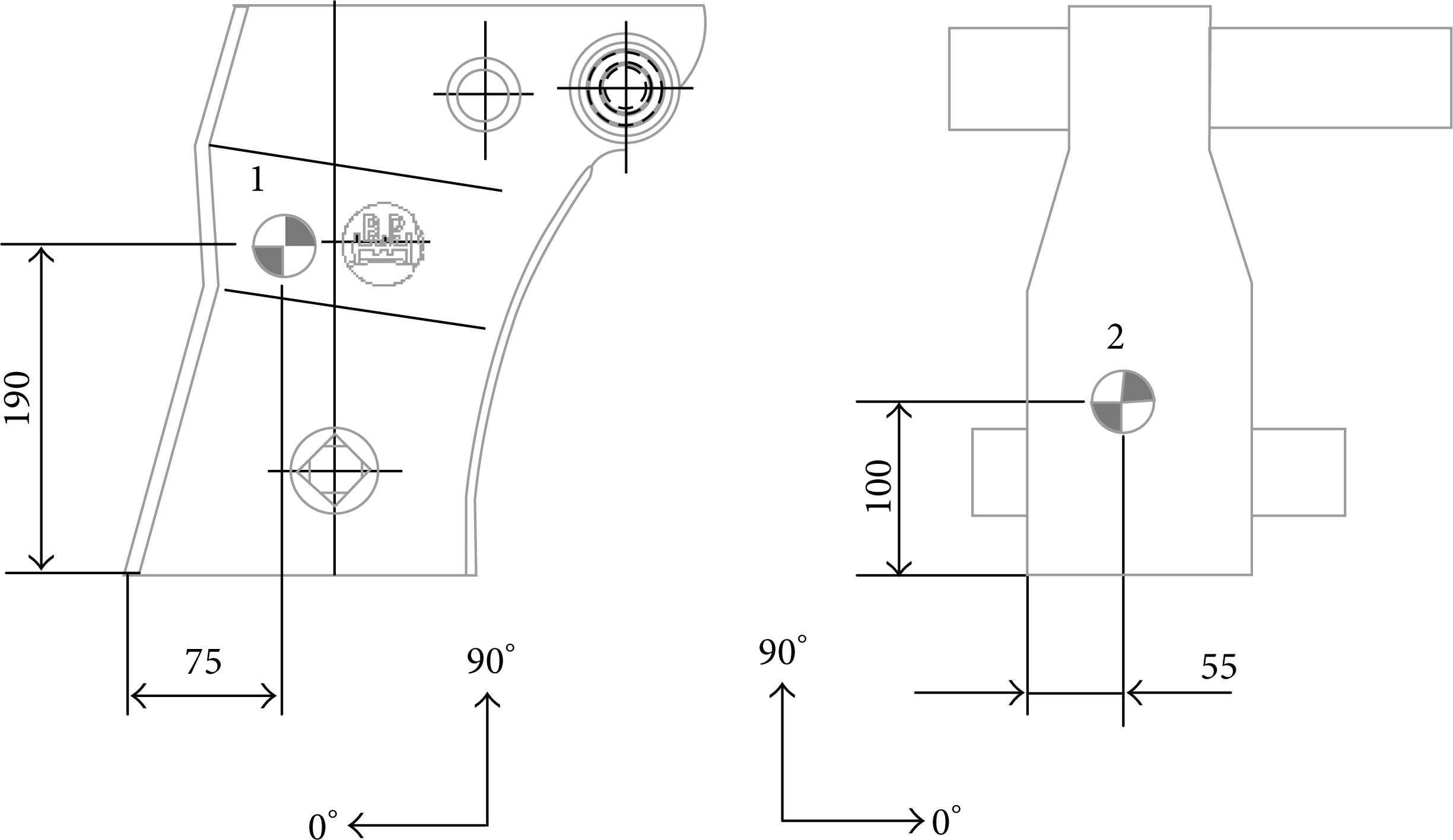
Location of strain gages 1 and 2 in the axle's support (mm).

The criterion followed in the selection of point locations for the strain gages was based on choosing these points in regions of the support's outer surface with stable values of stress and strain when the minimum radius manoeuvre load case takes place. Therefore, the stress and strain results in the support zone were previously assessed in the initial analyses. Additionally, these points had to be accessible enough to fix the gages adequately: the support was sanded in these points to remove the paint and then the strain gages were bonded to the support surface. The extensometric measurements were received in an 8-channel strain gage module DBK 43A [15], which provided eight channels of strain gage input and can accommodate most bridge-type sensors and load cells. Tests’ data were then saved in a laptop connected to the module, which could be adequately postprocessed with the software DASYLAB.

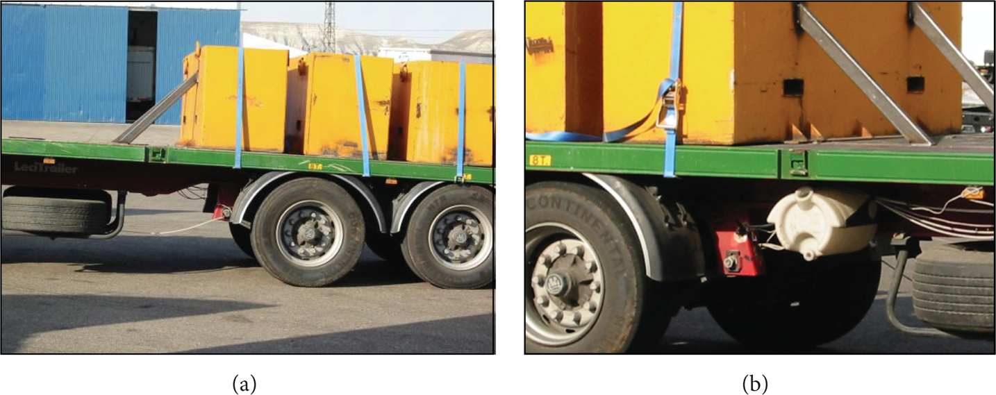
Figure 20(a) shows a detail of the loading process. Three masses with a weight of 9 tons each were lifted by an overhead travelling crane at LeciTrailer S.A. facilities and then adequately clamped over the semitrailer platform by means of steel beams, as shown in Figure 21, putting each one on top of each axle of the vehicle. As shown in Figure 20(b), the measurement equipment was located in the free space available at the front of the semitrailer platform.

Figure 20:

Loading and measurement equipment extensometric test of the vehicle.

Figure 21:

Mass assembly to the semitrailer platform.

Apart from the “minimum radius maneuver,” additional typical maneuvers such as braking and acceleration could also be tested in the semitrailer for further analysis. Figures 21 and 22 show several moments during the test. The evolution of the extensometric data values registered in the “minimum radius manoeuvre” was obtained in the postprocess and is shown in Figure 23.

Figure 22:

Extensometric test performed in a three-axle semitrailer.

Figure 23:

Strain evolution at gage 1 in the “minimum radius manoeuvre” performed during the test.

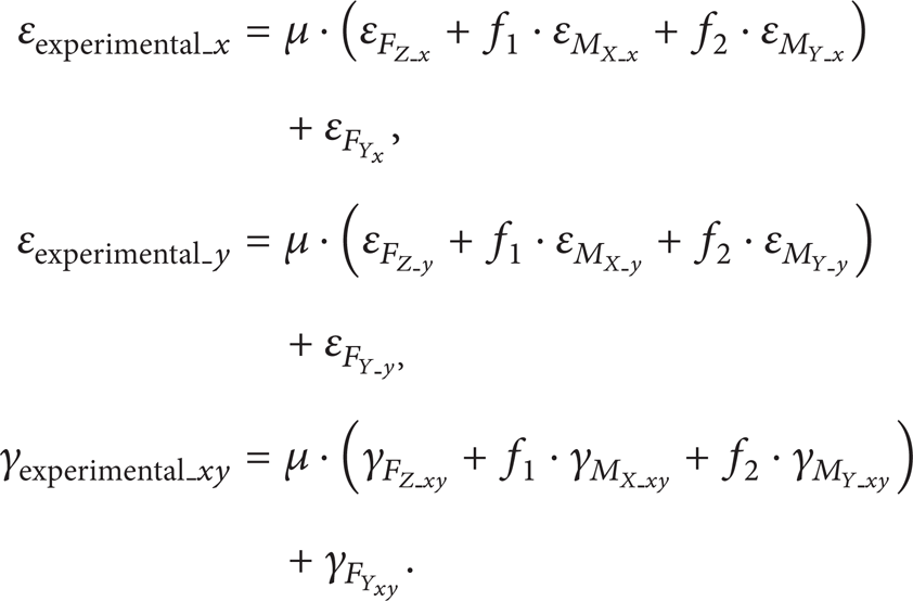
The strain values obtained in gage 1 are collected in Table 4. According to Figure 17, while ∊ _x and ∊ _y are obtained directly from the horizontal and vertical axis of the strain gages, strain values γ _xy can be calculated from the following equation:

${\gamma }_{xy}=\mathrm{2}·{\epsilon }_{{\mathrm{45}}^{°}}-{\epsilon }_x-{\epsilon }_y.$

(2)

Table 4:

Experimental strain values in gage 1.

Gage 1	Microstrain x-axis (∊ x )	−68,13
	Microstrain_y-axis (∊ y )	−73,87
	Microstrain 45° axis (∊45°)	324,20

5.3. Estimation of Load Parameters by means of Numerical-Experimental Data

Once numerical and experimental strain values were obtained for the support part (Tables 3 and 4), the following hypotheses were considered for loads F _z , M _x , and M _y :

• $\hspace{0.17em}\mu >\mathrm{1},$

  (3)

  which implies that the friction force required to slide the tyres along the road surface is greater than the normal force of the ground on the tyres; rubber surfaces on hard substrates can exhibit this behaviour due to internal friction and adhesion phenomena [16];

  $M_{x\_\text{transmitted}}=f_{\mathrm{1}}·M_{x\_\text{calculated}},$

  (4)

  where f₁ = flexibility coefficient for the calculated load M _x ;

• $M_{y\_\text{transmitted}}=f_{\mathrm{2}}·M_{y\_\text{calculated}},$

  (5)

  where f₂ = flexibility coefficient for the calculated load M _y ;

• the total strain components can be estimated applying the superposition principle to the strains components corresponding to each load applied independently;

• since the simulation strains were calculated for a friction coefficient μ = 1, the new friction coefficient estimated should also have an effect on the calculated moments M_{x_calculated} and M_{y_calculated} which are obtained from the friction force between the tyre and the ground.

Based on these hypotheses, the following equations have been created. This equation system combined the experimental and numerical data obtained to estimate the parameters μ, f₁, and f₂:

$\begin{array}{c}{\epsilon }_{\text{experimental}\_x}=\mu ·({\epsilon }_{F_{Z\_x}}+f_{\mathrm{1}}·{\epsilon }_{M_{X\_x}}+f_{\mathrm{2}}·{\epsilon }_{M_{Y\_x}})+{\epsilon }_{F_{Y_x}},\\ {\epsilon }_{\text{experimental}\_y}=\mu ·({\epsilon }_{F_{Z\_y}}+f_{\mathrm{1}}·{\epsilon }_{M_{X\_y}}+f_{\mathrm{2}}·{\epsilon }_{M_{Y\_y}})+{\epsilon }_{F_{Y\_y},}\\ {\gamma }_{\text{experimental}\_xy}=\mu ·({\gamma }_{F_{Z\_xy}}+f_{\mathrm{1}}·{\gamma }_{M_{X\_xy}}+f_{\mathrm{2}}·{\gamma }_{M_{Y\_xy}})+{\gamma }_{F_{Y_{xy}}}.\end{array}$

(6)

A sensitivity analysis of this equation system was carried out by means of the variation of f₁ factor (from 0 to 1), f₂ factor (from 0 to 0, 1), and the friction factor μ (from 1 to 1, 4) in order to minimize as much as possible the deviation values between the numerical and the experimental results in the equation system.

Finally, the optimal values for the load parameters were the following:

$\begin{array}{c}\mu =\mathrm{1,4},\\ f_{\mathrm{1}}=\mathrm{0,3},\\ f_{\mathrm{2}}=\mathrm{0,1}.\end{array}$

(7)

Once these parameters were estimated, it was possible to approximate the equivalent loads system that can be applied to the first axle's support structure in order to simulate the minimum radius manoeuvre. These loads are defined for a simultaneous application on both the right and left support parts as shown in Figures 13 and 14. The transmitted forces and moments reached the following values:

$\begin{array}{c}{F}_y=\mathrm{13.950}\hspace{0.17em}\text{N}\left(\text{Vertical}\right),\\ F_z=\mathrm{63.000}\hspace{0.17em}\text{N}\left(\text{Horizontal}\right),\\ M_x=\mathrm{6.200}\hspace{0.17em}\text{N}·\text{m}\left(\text{Horizontal}\hspace{0.17em}\hspace{0.17em}\text{axis}\right),\\ M_y=\mathrm{4.347}\hspace{0.17em}\text{N}·\text{m}\left(\text{Vertical}\hspace{0.17em}\hspace{0.17em}\text{axis}\right).\end{array}$

(8)

6. FE Simulation of the Initial Design of Axle's Support Structure

In the next step, the load system estimated in the previous point was applied to the FE model developed for the initial design of axle support structure. Figure 24 shows the Von Mises stress diagram obtained for the complete mesh model in the postprocess. The stress distributions on each one of the different areas of the model are detailed in Table 5, which points out the zones in the model reaching the maximum Von Mises stress values. The number of cycles for fatigue failure corresponding to these regions with maximum stress was then obtained according to Figure 11 and is also included in Table 5.

Table 5:

Maximum stress regions and results of the fatigue analysis with S-N curves.

Figure 24:

Von Mises stress distribution (MPa) for the axle's support structure.

As can be observed in Table 5, the most unfavorable regions with Von Mises stress values of 775 MPa were located in the welding points between the support and the lower transversal beam (concretely in the HAZ 1 of both the support and the lower transversal beam). According to this result, fatigue failure would appear at a low number of cycles in this zone (300 cycles). However, as the rest of the welding points presented much lower stress levels, their fatigue life was expected to be much longer and these results were considered acceptable. It has to be pointed out that a less conservative criterion in the S-N curves’ definition would have provided higher values in the number of cycles necessary to produce fatigue failure in the critical points (approximately 3000 cycles at the points with the maximum stress level in HAZ 1 if tensile strength would have been assigned a maximum value of 1000 cycles in the S-N curve).

7. Numerical Model Validation

In order to validate the FE numerical model used in this paper, a prototype of the axle's support structure of the vehicle was built. Then, it was assembled on a test bench provided with hydraulic cylinders and extensometric tests were carried out for several load cases in order to measure the strain values at two different measuring points located in the supports’ surfaces. These values were postcorrelated with theoretical values obtained in equivalent numerical simulations.

Concretely, the following two load cases were analysed.

1. Load case 1 consisted in the application of a force of 6.000 N in z-axis direction to both axle supports.

2. Load case 2 consisted in the application of a moment of 3.000 N·m in x-axis direction to both axle supports.

These load values were previously chosen taking into account initial numerical simulations where the structural behaviour was within the elastic range of steel. Therefore, all the steel parts of the prototype were expected to reach stress values much lower than their respective yield strengths and the same prototype could be used for different static tests, once it had recovered its initial shape.

Figure 25 shows a detail of the test bench with the hydraulic cylinders 1 and 2 and the prototype of the axle's support structure mounted upside down on it. Two extensometric gages were located, respectively, at the same points that were described in Figure 19. The test procedure and instrumentation were similar to the previous extensometric tests described in point 5.2.

Figure 25:

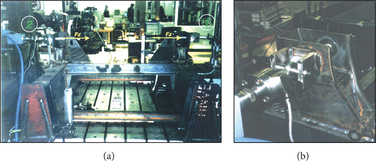
(a) Test bench disposition for test 1. (b) Hydraulic cylinder detail for force F _z application.

Figure 26:

Hydraulic cylinders positions in test 2 for the application of moment M _x .

Tables 6 and 7 show the experimental and numerical strain values that were obtained in load cases 1 (F _z ) and 2 (M _x ). The equivalent Von Mises stress values were also calculated from the experimental strain components with (9) [11, 14] and then could be compared to the numerical Von Mises stress values at the measuring points defined:

$\begin{array}{c}{\sigma }_{\mathrm{1,2}}=\frac{E}{(\mathrm{1}-\nu )}·\frac{{\epsilon }_x+{\epsilon }_y}{\mathrm{2}}\pm \frac{E}{\sqrt{\mathrm{2}}·\left(\mathrm{1}+\nu \right)}·\sqrt{{\left({\epsilon }_x-{\epsilon }_{{\mathrm{45}}^{°}}\right)}^{\mathrm{2}}+{\left({\epsilon }_y-{\epsilon }_{{\mathrm{45}}^{°}}\right)}^{\mathrm{2}}},\\ {\sigma }_{\text{VM}}=\sqrt{{\sigma }_{\mathrm{1}}^{\mathrm{2}}+{\sigma }_{\mathrm{2}}^{\mathrm{2}}-{\sigma }_{\mathrm{1}}·{\sigma }_{\mathrm{2}},}\end{array}$

(9)

where σ_VM = equivalent Von Mises planar stress, σ_1,2 = principal stresses for linear, isotropic, and homogeneous material, ν = Poisson's ratio, and E = Young's modulus.

Table 6:

Numerical-experimental strain and stress comparison for load case 1 (F _z ).

Fz horizontal load case	∊ x (μ∊)	∊ y (μ∊)	∊45° (μ∊)	Von Mises stress (MPa)
Gage 1
Numerical values	−7,3	3,5	−10	2,7
Experimental values	−9	1	−22	5,3
Gage 2
Numerical values	−14,3	7	34	11,0
Experimental values	−14	6	40	12,7

Table 7:

Numerical-experimental strain and stress comparison for load case 2 (M _x ).

Mx horizontal load case	∊ x (μ∊)	∊ y (μ∊)	∊45° (μ∊)	Von Mises stress (MPa)
Gage 1
Numerical values	−15	−72	−130,5	28,7
Experimental values	60	−95	−130	38,6
Gage 2
Numerical values	−36,4	16	38	15,6
Experimental values	−36	15	75	25,1

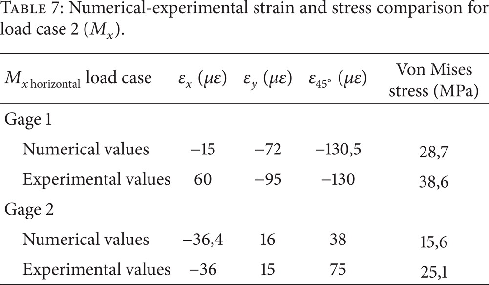
As can be observed in Tables 6 and 7, except for inaccuracies detected in several values, numerical and experimental values showed in general an adequate correlation level. As a result of this, the numerical models used in this analysis were considered accurate enough to carry out the loads estimation described in point 5.3.

8. Improvement on the Initial Structure

Once the loads acting on the structure were estimated, the numerical analysis was performed and the fatigue life of the initial design was assessed; a modification in the most critical area resulting from the fatigue analysis with S-N curves described in point 6 could be proposed. Concretely, it was considered to change the lower transversal beam for another one with a higher cross-sectional area in order to obtain a higher length of welding bead and to reduce the stress levels reached at the welded joint area with the supports. Figure 27 shows the new design proposed for the lower transversal beam.

Figure 27:

Improvement proposed in the cross-section of the lower transversal beam.

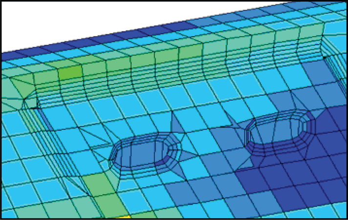
This modification was included in the numerical model and then it was analyzed in a new iteration. The new Von Mises stress results for the structure are shown in Figure 28 (MPa) and a detail of the welded joint between the lower transversal beam and one of the supports can be observed in Figure 29. Finally, the updated values of expected fatigue life (cycles) were obtained according to the S-N curves previously defined and are shown in Table 8.

Table 8:

Results in the joint zone between the support and the lower transversal beam.

Material	Maximum Von Mises stress (Mpa)	Failure cycles
Weld bead	617	8.000
HAZ 1	771	400
HAZ 2	689	600
HAZ 3	649	700

Figure 28:

Von Mises stress distribution for the whole modified structure (MPa).

Figure 29:

Detail of the Von Mises stress distribution for the welded joint between the new design of lower transversal beam and the support (MPa).

With the improvement proposed, a significant reduction of the maximum stress values was achieved, reaching almost a 50% reduction in some points, and the expected fatigue life of the structure could be improved. Particularly, the most critical point of the model (the HAZ 1 at the welded joint between the support and the lower transversal beam) showed an increase of its fatigue life from 300 to 400 cycles.

9. Concluding Remarks

As a result of the numerical-experimental method developed in this paper, the fatigue behaviour of the structure of a semitrailer's axle support could be assessed. The result of this analysis was the maximum number of load cycles that the structure can overcome till a fatigue failure takes place, with each load cycle corresponding to the forces and moments acting on the structure when the semitrailer is performing the “minimum radius manoeuvre” with a transported load of 27 tons.

The combination of numerical and experimental data made it possible to estimate this critical load state, and then the structure could be analyzed by means of the simulation of FE numerical models that were also experimentally correlated. Moreover, the weld beads and the HAZs of the structure were also included in the numerical models, which supposed not only the definition of their mechanical properties by means of hardness tests but also a higher accuracy of the numerical models.

Finally, some dimensional changes were proposed on the initial design of the axle's support structure in order to improve its fatigue behavior.

It can be concluded that the application of this method is able to assess the fatigue behaviour of semitrailers at critical areas. This will allow manufacturers to develop new semitrailer structural designs with a higher operational lifespan and able to withstand the minimum radius manoeuvre without failure.

Conflict of Interests

The authors declare that there is no conflict of interests regarding the publication of this paper.