An Observer-Based Adaptive Iterative Learning Control Using Filtered-FNN Design for Robotic Systems

Abstract

An observer-based adaptive iterative learning control using a filtered fuzzy neural network is proposed for repetitive tracking control of robotic systems. A state tracking error observer is introduced to design the iterative learning controller using only the measurement of joint position. We first derive an observation error model based on the state tracking error observer. Then, by introducing some auxiliary signals, the iterative learning controller is proposed based on the use of an averaging filter. The main control force consists of a filtered fuzzy neural network used to approximate for unknown system nonlinearity, a robust learning term used to compensate for uncertainty, and a stabilization term used to guarantee the boundedness of internal signals. The adaptive laws combining time domain and iteration domain adaptation are presented to ensure the convergence of learning error. We show that all the adjustable parameters as well as internal signals remain bounded for all iterations. The norm of output tracking error will asymptotically converge to a tunable residual set as iteration goes to infinity.

1. Introduction

Due to the repeatability of operation for robotic systems, it is suitable to perform the control task by using the technique of iterative learning control (ILC) for a repetitive tracking control problem. ILC is basically a non-model-based learning approach which is very effective in dealing with repetitive control tasks [1–5]. Initially, PID-type ILC algorithms which required a certain a priori knowledge of robot dynamics were developed for robot manipulators based on the contraction mapping theory [6–9]. In D-type, PD-type, or PID-type ILC, the acceleration errors of joint variables are required to construct the learning controller. However, the acceleration measurement is unfortunately not realizable in practice and becomes the major disadvantage of D-type ILC. On the other hand, P-type ILC uses only the velocity errors of joint variables for the design of updated learning function. Although the requirement of acceleration measurement is removed, more strict conditions on the robot manipulators are needed for technical analysis. In general, it is hard to apply the traditional PID-type ILC for repetitive tracking control of robot manipulator using only joint position measurement.

Recently, adaptive iterative learning control (AILC) has been widely studied in the research field of the ILC. One of the most attractive advantages of AILC scheme is the capability to deal with the issues of large initial resetting error, large input disturbance, and iteration-varying desired trajectory. In the past decade, the AILC schemes have been utilized for repeated tracking control of robotic systems [10–14], or a class of nonlinear systems [15, 16]. In order to relax the restrict Lipschitz condition on the plant's nonlinearity, the Lyapunov-like approach instead of contraction mapping theory is applied in AILC to analyze the stability and convergence. If the system nonlinearties are unknown, the fuzzy systems or neural networks were often introduced to approximate the nonliearties and provide the basis functions for the design of AILC [17–19]. However, both PID-type ILCs and AILCs require at least the joint velocities to develop the AILC algorithms. If only the measurement of joint positions is available, an observer is one of the possible choice to design the AILC. In [20], an observer-based ILC for a time-varying nonlinear system was proposed to overcome the unmeasurable states. Although an observer-based ILC system can guarantee that the tracking error will converge to zero, the initial resetting errors at each iteration were not considered. In [21], an observer-based ILC scheme was proposed for a class of nonlinear systems with unknown parametric uncertainties. The Lyapunov-Krasovskii-like composite energy function was applied to analyze the closed-loop stability and learning performance. Nevertheless, the plant nonlinearities must be linearly parameterizable. In [22], a framework for ILC by using an observer to estimate the controlled variable was presented. However, it was necessary to assume that the ILC input converges to a bounded signal. In [23], the observer-based ILC with evolutionary programming algorithm was proposed for MIMO nonlinear systems. The evolutionary programming was applied to search for the optimal and feasible learning gain to speed up the convergence of the ILC and the tracking error will converge to zero via successive learning. But the AILC was developed for MIMO nonlinear plants with nonlinearities satisfying Lipschitz continuous condition. In [24], an observer-based AILC was developed for a class of nonlinear systems with unknown time-varying parameters and unknown time-varying delays. The linear matrix inequality (LMI) approach was used to design the nonlinear state observer. By constructing a Lyapunov-Krasovskii-like composite energy function, the boundedness of the internal signals and the convergence of tracking error can be proved. However, it was assumed that the plant nonlinearities satisfy Lipschitz continuous condition and the unknown system parameters must be linear with respect to some known nonlinear vector-valued functions. In [25], a velocity-observer-based ILC for trajectory tracking of rigid robot manipulators with external disturbances without using the velocity measurement was proposed. However, the inertia matrix of the robotic systems needed to satisfy Lipschitz continuous condition and the initial resetting errors at each iteration were assumed to be zero. Besides, the disturbances were assumed to be repetitive and the velocities were assumed to be bounded.

In order to relax the condition of measurement for joint velocity and without the requirement of Lipschitz condition on the robot unknown nonlinearity and the zero initial resetting errors at each iteration, a new observer-based adaptive iterative learning controller using a new filtered fuzzy neural network (filtered-FNN) is proposed for repetitive tracing control of robotic systems in this paper. A state tracking error observer is firstly presented to deal with the problem that only joint positions are available. Based on this observer, a state tracking error model including a filtered-FNN approximation term can be derived by using an interesting s-domain transfer function technique which is usually utilized in the area of traditional model reference adaptive control [26]. An averaging filter is then proposed to solve the implementation problem of the controller. Under the derived error model, a fuzzy neural learning component is designed to approximate the unknown nonlinearities by a filtered-FNN using state estimation vector as the network input, a robust learning component is constructed to compensate for the uncertainties from approximation error and state estimation error, and a stabilization component is used to guarantee the boundedness of internal signals. The main features of this iterative learning controller and its contributions relative to the related works are summarized as follows.

1. Compared with most of the works using adaptive iterative learning control for robotic systems or nonlinear systems, this paper can design a realizable adaptive iterative learning controller using only joint position measurement. In other words, it is not necessary to measure the states for the controller design.

2. A new design approach is introduced to derive the error model so that a filtered-FNN can be applied for compensation of the unknown system nonlinearities. The filtered-FNN can be treated as a dynamic version of traditional FNN which plays an important role in this proposed adaptive iterative learning controller.

3. Compared with the fuzzy system or neural-network-based adaptive iterative learning controller using state measurement [17–19], the stability analysis becomes more difficult since the boundedness of output tracking error cannot guarantee the boundedness of input signal. A new analysis to prove the regularity of internal signals is successfully derived in this paper so that we ensure the boundedness of all the adjustable parameters and internal signals during the learning process. Furthermore, we guarantee that the norm of output tracking error will asymptotically converge to a tunable residual set which depends on the design parameters if iteration number is large enough.

This paper is organized as follows. In Section 2, a problem formulation is given. The error model between system output and desired output is derived in Section 3. Based on the derived error model, the filtered-FNN-based AILC using observer design is presented in Section 4. Analysis of closed-loop Section 6. The detailed description of the proposed filtered FNN is given in the Appendix.

In the subsequent discussions, the following notations will be used.

1. $\left|\hspace{0.17em}·\hspace{0.17em}\right|$ denotes the absolute value of a scalar or the Euclidean or any other consistent norm of a vector or matrix.

2. L _pe [0,T] denotes the set of Lebesgue measurable (or piecewise continuous) real-valued (vector) functions with

   $\mathrm{\hspace{0.17em}\hspace{0.17em}}{\left|·\right|}_{pe}=\{\begin{array}{cc}{\left({{\displaystyle \int }}_{\mathrm{0}}^T‍{\left|·\right|}^{p}dt\right)}^{\mathrm{1}/p},\hfill & \text{if}\hspace{0.17em}p\in \left[\mathrm{1},\infty \right),\hfill \\ \underset{\mathrm{0}\le t\le T}{\sup }\left|·\right|,\hfill & \text{if}\hspace{0.17em}p=\infty .\hfill \end{array}$

   (1)

3. ${\parallel {(·)}_t\parallel }_{\infty }={\sup }_{\tau \le t}\left|(·)(\tau )\right|$ denotes the truncated L_∞ norm of the argument function or vector [26].

4. ${\parallel G(s)\parallel }_{\infty }$ denotes the H_∞ norm of the transfer function G(s).

5. G(s)[u(t)] denotes the filtered version of u(t) with any proper or strictly proper transfer function G(s).

2. Problem Formulation

In this paper, we consider an uncertain robotic system with n rigid bodies which can perform a given task repeatedly over a finite time interval [0,T] as follows:

$D\left(q^j\left(t\right)\right){\ddot{q}}^j\left(t\right)+B\left(q^j\left(t\right),{\dot{q}}^j\left(t\right)\right){\dot{q}}^j\left(t\right)+F\left(q^j\left(t\right),{\dot{q}}^j\left(t\right)\right)=u^j\left(t\right),$

(2)

where j∈Z_/+ denotes the index of iteration number and t∈[0,T] denotes the time index. The signals q ^j (t), ${\dot{q}}^j(t)$ , ${\ddot{q}}^j(t)\in {ℛ}^{n\times \mathrm{1}}$ are, respectively, the generalized joint position, joint velocity, and joint acceleration vectors. D(q ^j (t))∈ℛ^{n × n} is the inertia matrix, $B(q^j(t),\hspace{0.17em}\hspace{0.17em}{\dot{q}}^j(t))\in {ℛ}^{n\times n}$ is the centripetal plus Coriolis force matrix, $F(q^j(t),\hspace{0.17em}\hspace{0.17em}{\dot{q}}^j(t))\in {ℛ}^{n\times \mathrm{1}}$ are the gravitational plus frictional forces, and u ^j ∈ ℛ^{n × 1} is the joint torque vector. It is noted the inertia matrix D(q ^j (t)) is assumed to be positive definite and bounded for all t∈[0,T] and iteration j≥1 as

$\mathrm{0}<m_{\mathrm{1}}{I}_{n\times n}\le D\left(q^j\left(t\right)\right)\le m_{\mathrm{2}}{I}_{n\times n},$

(3)

where m₁,m₂>0 and I_{n × n} is an n × n identity matrix. Since the inverse of inertia matrix exists for all joint variables, the dynamic formulation of the robotic system can be written as follows:

$\begin{array}{c}{\ddot{q}}^j\left(t\right)=-D^{-\mathrm{1}}\left(q^j\left(t\right)\right)\\ \hspace{1em}\times \left[B\left(q^j\left(t\right),{\dot{q}}^j\left(t\right)\right){\dot{q}}^j\left(t\right)+F\left(q^j\left(t\right),{\dot{q}}^j\left(t\right)\right)\right]\\ \hspace{1em}\hspace{1em}\hspace{1em}+D^{-\mathrm{1}}\left(q^j\left(t\right)\right)u^j\left(t\right).\end{array}$

(4)

Let $f(q^j(t),{\dot{q}}^j(t))=D^{-\mathrm{1}}(q^j(t))[B(q^j(t),{\dot{q}}^j(t)){\dot{q}}^j(t)+F(q^j(t),{\dot{q}}^j(t))]\in {ℛ}^{n\times \mathrm{1}}$ and b(q ^j (t)) = D⁻¹(q ^j (t))∈ℛ^{n × n} and choose the output variable as y ^j (t) = q ^j (t)∈ℛ^{n × 1}, state variable as $X^j(t)={[x_{\mathrm{1}}^j{(t)}^{\top },\hspace{0.17em}\hspace{0.17em}{x}_{\mathrm{2}}^j{(t)}^{\top }]}^{\top }={[y^j{(t)}^{\top },\hspace{0.17em}\hspace{0.17em}{\dot{y}}^j{(t)}^{\top }]}^{\top }={[q^j{(t)}^{\top },\hspace{0.17em}\hspace{0.17em}{\dot{q}}^j{(t)}^{\top }]}^{\top }\in {ℛ}^{\mathrm{2}n\times \mathrm{1}}$ , then we have

$\begin{array}{c}{\dot{x}}_{\mathrm{1}}^j\left(t\right)=x_{\mathrm{2}}^j\left(t\right),\\ {\dot{x}}_{\mathrm{2}}^j\left(t\right)=-f\left(X^j\left(t\right)\right)+b\left(X^j\left(t\right)\right)u^j\left(t\right),\\ y^j\left(t\right)=x_{\mathrm{1}}^j\left(t\right),\end{array}$

(5)

or equivalently in the following state-space form:

$\begin{array}{c}{\dot{X}}^j\left(t\right)=A{X}^j\left(t\right)+B\left(-f\left(X^j\left(t\right)\right)+b\left(X^j\left(t\right)\right)u^j\left(t\right)\right),\\ y^j\left(t\right)=C^{\top }{X}^j\left(t\right),\end{array}$

(6)

where

$A=\left[\begin{array}{cc}\mathrm{0}& I_{n\times n}\\ \mathrm{0}& \mathrm{0}\end{array}\right]\in {ℛ}^{\mathrm{2}n\times \mathrm{2}n},\hspace{1em}\hspace{1em}B=\left[\begin{array}{c}\mathrm{0}\\ I_{n\times n}\end{array}\right]\in {ℛ}^{\mathrm{2}n\times n},\begin{array}{c}C=\left[\begin{array}{c}{I}_{n\times n}\\ \mathrm{0}\end{array}\right]\in {ℛ}^{\mathrm{2}n\times n},\end{array}$

(7)

Here, 0<b(X ^j (t)) ≤ m₁⁻¹I_{n × n}. In this paper, we assume that only joint position y ^j (t) = q ^j (t) is measurable for controller design. Let the signals q _d (t), ${\dot{q}}_d(t)$ , ${\ddot{q}}_d(t)\in {ℛ}^{n\times \mathrm{1}}$ be, respectively, the desired generalized joint position, joint velocity, and joint acceleration vectors; the desired state trajectory can be defined as $X_d(t)={[x_{d_{\mathrm{1}}}{(t)}^{\top },\hspace{0.17em}\hspace{0.17em}{x}_{d_{\mathrm{2}}}{(t)}^{\top }]}^{\top }={[y_d{(t)}^{\top },{\dot{y}}_d{(t)}^{\top }]}^{\top }={[q_d{(t)}^{\top },{\dot{q}}_d{(t)}^{\top }]}^{\top }$ . Now, given a specified desired output trajectory y _d (t), t∈[0,T] and an initial desired output y _d (0)≠y ^j (0) for all j≥1, the control objective for the robotic systems executing a repeatable task is to force the output y ^j (t) to follow y _d (t) as close as possible.

3. Derivations of Error Model and Controller

3.1. Derive the Error Model

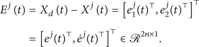
Define an output tracking error as e ^j (t) = y _d (t)-y ^j (t) and state tracking errors as e₁ ^j (t) = y _d (t)-y ^j (t), $e_{\mathrm{2}}^j(t)={\dot{y}}_d(t)-{\dot{y}}^j(t)$ . It is assumed that the initial output tracking error vector at each iteration is not necessarily zero, small, and fixed but satisfies $\left|e^j(\mathrm{0})\right|={\varepsilon }^j$ for a known positive constants ɛ ^j since the joint position vector y ^j (t) is measurable. Let the state tracking error vector be defined as

$E^j\left(t\right)=X_d\left(t\right)-X^j\left(t\right)={\left[e_{\mathrm{1}}^j{\left(t\right)}^{\top },e_{\mathrm{2}}^j{\left(t\right)}^{\top }\right]}^{\top }={\left[e^j{\left(t\right)}^{\top },{\dot{e}}^j{\left(t\right)}^{\top }\right]}^{\top }\in {ℛ}^{\mathrm{2}n\times \mathrm{1}}.$

(8)

Then we can derive ${\ddot{e}}^j(t)$ as follows:

${\ddot{e}}^j\left(t\right)={\ddot{y}}_d\left(t\right)+f\left(X^j\left(t\right)\right)-b\left(X^j\left(t\right)\right)u^j\left(t\right)=-K_c^{\top }{E}^j\left(t\right)+f\left(X^j\left(t\right)\right)+{\ddot{y}}_d\left(t\right)+K_c^{\top }{E}^j\left(t\right)-b\left(X^j\left(t\right)\right)u^j\left(t\right),$

(9)

where K _c = [k₂ ^c I,k₁ ^c I]^⊤ ∈ ℛ^{2n × n} is a feedback gain matrix such that the characteristic polynomial of A _c = A-BK _c ^⊤ is Hurwitz. Therefore, the tracking error dynamics will satisfy

$\begin{array}{c}{\dot{E}}^j\left(t\right)\\ =A_c{E}^j\left(t\right)+B[\phantom{K_c^{\top }{E}^j\left(t\right)-b\left(X^j\left(t\right)\right)u^j\left(t\right)}f\left(X^j\left(t\right)\right)+{\ddot{y}}_d\left(t\right)+K_c^{\top }{E}^j\left(t\right)-b\left(X^j\left(t\right)\right)u^j\left(t\right)]\\ =A_c{E}^j\left(t\right)+B[\phantom{\left(\mathrm{1}-b\left(X^j\left(t\right)\right)\right)}\phantom{\left(\mathrm{1}-b\left(X^j\left(t\right)\right)\right)}f\left(X^j\left(t\right)\right)+{\ddot{y}}_d\left(t\right)+K_c^{\top }{X}_d\left(t\right)-K_c^{\top }{X}^j\left(t\right)-u^j\left(t\right)+\left(\mathrm{1}-b\left(X^j\left(t\right)\right)\right)u^j\left(t\right)],\\ =A_c{E}^j\left(t\right)+B\left[h\left(X^j\left(t\right)\right)-u^j\left(t\right)+\left(\mathrm{1}-b\left(X^j\left(t\right)\right)\right)u^j\left(t\right)\right],\\ e^j\left(t\right)=C^{\top }{E}^j\left(t\right),\end{array}$

(10)

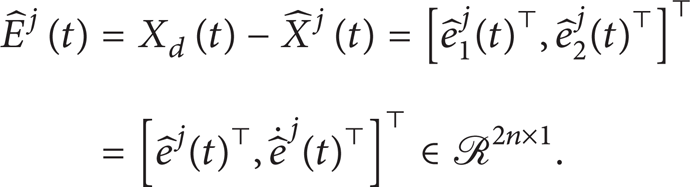
where $h(X^j(t))\equiv f(X^j(t))-K_c^{\top }{X}^j(t)+{\ddot{y}}_d(t)+K_c^{\top }{X}_d(t)$ . Note that the state tracking error vector E ^j (t) in the tracking error dynamics (10) is not assumed to be available for measurement. Hence, it is necessary to construct a state estimation vector ${\widehat{X}}^j(t)={[{\widehat{x}}_{\mathrm{1}}^j{(t)}^{\top },{\widehat{x}}_{\mathrm{2}}^j{(t)}^{\top }]}^{\top }={[{\widehat{y}}^j{(t)}^{\top },{\dot{\widehat{y}}}^j{(t)}^{\top }]}^{\top }\in {ℛ}^{\mathrm{2}n\times \mathrm{1}}$ for estimation of the state vector. In order to construct a state estimation vector, we first define an output tracking error estimation vector as ${\widehat{e}}^j(t)=y_d(t)-{\widehat{y}}^j(t)$ . Then the state tracking error estimation vector can be defined as

${\widehat{E}}^j\left(t\right)=X_d\left(t\right)-{\widehat{X}}^j\left(t\right)={\left[{\widehat{e}}_{\mathrm{1}}^j{\left(t\right)}^{\top },{\widehat{e}}_{\mathrm{2}}^j{\left(t\right)}^{\top }\right]}^{\top }={\left[{\widehat{e}}^j{\left(t\right)}^{\top },{\dot{\widehat{e}}}^j{\left(t\right)}^{\top }\right]}^{\top }\in {ℛ}^{\mathrm{2}n\times \mathrm{1}}.$

(11)

The state tracking error observer is designed as

$\begin{array}{c}{\dot{\widehat{E}}}^j\left(t\right)=A_c{\widehat{E}}^j\left(t\right)+K_o\left(e^j\left(t\right)-{\widehat{e}}^j\left(t\right)\right),\hspace{1em}{\widehat{E}}^j\left(\mathrm{0}\right)=\mathrm{0},\\ {\widehat{e}}^j\left(t\right)=C^{\top }{\widehat{E}}^j\left(t\right),\end{array}$

(12)

where K _o = [k₁ ^o I,k₂ ^o I]^⊤ ∈ ℛ^{2n × n} is the observer gain vector such that the characteristic polynomial of A _o = A _c -K _o C^⊤ is Hurwitz. Define an output observation error vector as ${\tilde{e}}^j(t)=e^j(t)-{\widehat{e}}^j(t)$ . Then the state observation error vector can be defined as

${\tilde{E}}^j\left(t\right)\mathrm{\hspace{0.17em}\hspace{0.17em}}=E^j\left(t\right)-{\widehat{E}}^j\left(t\right)={\left[{\tilde{e}}_{\mathrm{1}}^j{\left(t\right)}^{\top },{\tilde{e}}_{\mathrm{2}}^j{\left(t\right)}^{\top }\right]}^{\top }={\left[e^j{\left(t\right)}^{\top }-{\widehat{e}}^j{\left(t\right)}^{\top },{\dot{e}}^j{\left(t\right)}^{\top }-{\dot{\widehat{e}}}^j{\left(t\right)}^{\top }\right]}^{\top }\in {ℛ}^{\mathrm{2}n\times \mathrm{1}}.$

(13)

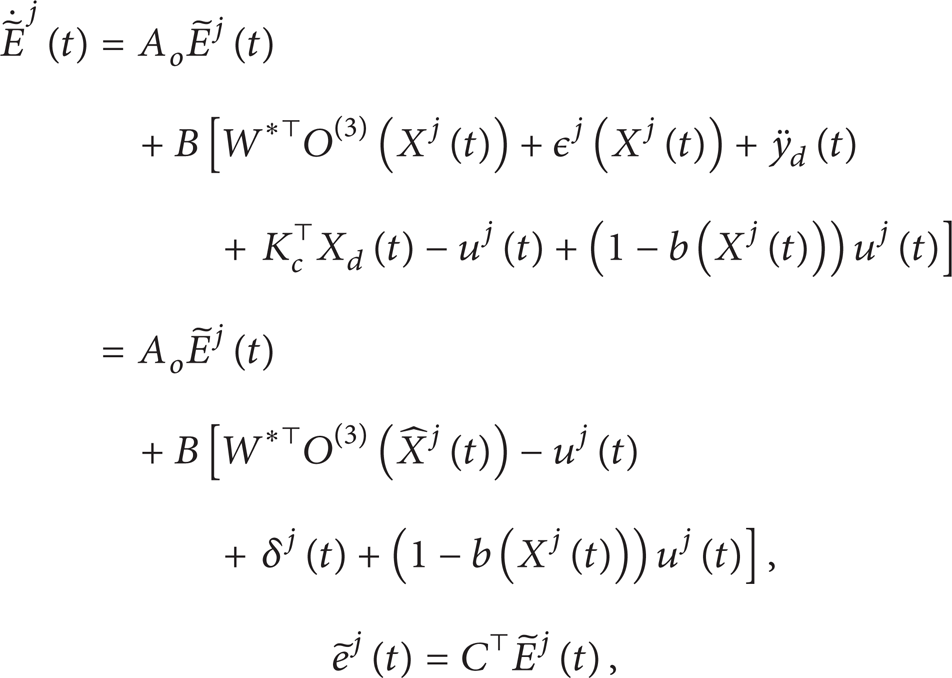
By using (10) and (12), we have the following observation error dynamics:

$\begin{array}{c}{\dot{\tilde{E}}}^j\left(t\right)=A_o{\tilde{E}}^j\left(t\right)+B\left[h\left(X^j\left(t\right)\right)-u^j\left(t\right)+\left(\mathrm{1}-b\left(X^j\left(t\right)\right)\right)u^j\left(t\right)\right],\\ {\tilde{e}}^j\left(t\right)=C^{\top }{\tilde{E}}^j\left(t\right).\end{array}$

(14)

Note that $\left|{\tilde{e}}^j(\mathrm{0})\right|=|e^j(\mathrm{0})-{\widehat{e}}^j(\mathrm{0})|=|e^j(\mathrm{0})|={\varepsilon }^j$ . Based on the universal approximation theorem, we know that the nonlinear function h(X ^j (t)) can be approximated by a traditional FNN [19] W ^j (t)^⊤O⁽³⁾(X ^j (t)). Here O⁽³⁾(X ^j (t))∈ℛ^{M × 1} is the basis function vector with M being the number of rule nodes and W ^j (t)∈ℛ^{M × n} is the weight matrix of the output layer. According to the universal approximation theorem, there will exist an optimal weight matrix W^* such that h(X ^j (t)) = W^*⊤O⁽³⁾(X ^j (t)) + ϵ(X ^j (t)), where ϵ(X ^j (t)) is the approximation error satisfying |ϵ(X ^j (t))| ≤ ϵ^* in a certain compact set. This implies that (14) can be rewritten as

$\begin{array}{c}{\dot{\tilde{E}}}^j\left(t\right)=A_o{\tilde{E}}^j\left(t\right)+B[\phantom{\left(\mathrm{1}-b\left({\text{X}}^j\left(t\right)\right)\right)}{W}^{*\top }{O}^{\left(\mathrm{3}\right)}\left(X^j\left(t\right)\right)+{ϵ}^j\left(X^j\left(t\right)\right)+{\ddot{y}}_d\left(t\right)+K_c^{\top }{X}_d\left(t\right)-u^j\left(t\right)+\left(\mathrm{1}-b\left(X^j\left(t\right)\right)\right)u^j\left(t\right)]=A_o{\tilde{E}}^j\left(t\right)+B[W^{*\top }{O}^{\left(\mathrm{3}\right)}\left({\widehat{X}}^j\left(t\right)\right)-u^j\left(t\right)+{\delta }^j\left(t\right)+\left(\mathrm{1}-b\left(X^j\left(t\right)\right)\right)u^j\left(t\right)],\\ {\tilde{e}}^j\left(t\right)=C^{\top }{\tilde{E}}^j\left(t\right),\end{array}$

(15)

where ${\delta }^j(t)=W^{*\top }(O^{(\mathrm{3})}(X^j(t))-O^{(\mathrm{3})}({\widehat{X}}^j(t)))+ϵ(X^j(t))$ is the lumped uncertainty term which includes the difference between FNN networks with input using state X ^j (t) and estimated state ${\widehat{X}}^j(t)$ and the network approximation error. It is easily proven that the lumped uncertainty term satisfies |δ ^j (t)| ≤ δ^*. However, it is noted that the value of the unknown constant δ^* might be large.

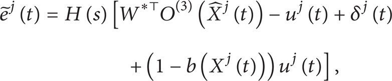
To see how to design the iterative learning controller u ^j (t) to achieve the control objective, we now adopt the mixed use of a time signal and a Laplace transfer function to obtain the explicit expression of ${\tilde{e}}^j(t)$ in (15) in time domain with a filtered version as follows:

${\tilde{e}}^j\left(t\right)=H\left(s\right)[W^{*\top }{O}^{\left(\mathrm{3}\right)}\left({\widehat{X}}^j\left(t\right)\right)-u^j\left(t\right)+{\delta }^j\left(t\right)+\left(\mathrm{1}-b\left(X^j\left(t\right)\right)\right)u^j\left(t\right)],$

(16)

where $H(s)=C^{\top }{(sI-A_o)}^{-\mathrm{1}}B=(\mathrm{1}/(s^{\mathrm{2}}+(k_{\mathrm{1}}^c+k_{\mathrm{1}}^o)s+(k_{\mathrm{1}}^c{k}_{\mathrm{1}}^o+k_{\mathrm{2}}^c{k}_{\mathrm{2}}^o)))I_{n\times n}$ . The observer gain vector K _o = [k₁ ^o I_{n × n},k₂ ^o I_{n × n}]^⊤ is chosen such that $H(s)=(\mathrm{1}/\ell (s)L(s))I_{n\times n}$ with ℓ(s) = s + λ and L(s) being any Hurwitz polynomial of order 1. Then (16) can be rewritten as

$\begin{array}{c}{\tilde{e}}^j\left(t\right)\\ =H\left(s\right)L\left(s\right)[W^{*\top }\frac{\mathrm{1}}{L\left(s\right)}\left[O^{\left(\mathrm{3}\right)}\left({\widehat{X}}^j\left(t\right)\right)\right]-\frac{\mathrm{1}}{L\left(s\right)}\left[u^j\left(t\right)\right]+\frac{\mathrm{1}}{L\left(s\right)}\left[\left(\mathrm{1}-b\left(X^j\left(t\right)\right)\right)u^j\left(t\right)+{\delta }^j\left(t\right)\right]]\\ =\frac{\mathrm{1}}{\ell \left(s\right)}[W^{*\top }\frac{\mathrm{1}}{L\left(s\right)}\left[O^{\left(\mathrm{3}\right)}\left({\widehat{X}}^j\left(t\right)\right)\right]-\frac{\mathrm{1}}{L\left(s\right)}\left[u^j\left(t\right)\right]+{\delta }_L^j\left(t\right)],\end{array}$

(17)

where ${\delta }_L^j(t)=(\mathrm{1}/L(s))[(\mathrm{1}-b(X^j(t)))u^j(t)+{\delta }^j(t)]$ .

3.2. Construct Some Useful Signals

According to the filtered version of output tracking error model (17), we define an augmented signal with filtered version as

$y_a^j\left(t\right)=\frac{\mathrm{1}}{\ell \left(s\right)}\left[v^j\left(t\right)-\frac{\mathrm{1}}{L\left(s\right)}\left[u^j\left(t\right)\right]\right],\hspace{1em}{y}_a^j\left(\mathrm{0}\right)=\mathrm{0},$

(18)

where v ^j (t) is an auxiliary input to be designed later. Then, design an auxiliary error signal as

$e_a^j\left(t\right)={\tilde{e}}^j\left(t\right)-y_a^j\left(t\right).$

(19)

The initial condition e _a ^j (0) will satisfy $|e_a^j(\mathrm{0})|=|{\tilde{e}}^j(\mathrm{0})-y_a^j(\mathrm{0})|=|{\tilde{e}}^j(\mathrm{0})|=|e^j(\mathrm{0})|\equiv {\varepsilon }^j$ . Substituting (17) and (18) into (19), we can find that

$e_a^j\left(t\right)={\tilde{e}}^j\left(t\right)-y_a^j\left(t\right)=\frac{\mathrm{1}}{\ell \left(s\right)}\left[W^{*\top }\frac{\mathrm{1}}{L\left(s\right)}\left[O^{\left(\mathrm{3}\right)}\left({\widehat{X}}^j\left(t\right)\right)\right]-v^j\left(t\right)+{\delta }_L^j\left(t\right)\right].$

(20)

It is noted that we apply the Laplace operation to derive the tracking error model (20) for technical analysis later as that used in the traditional model reference adaptive control [26]. The equivalent time-domain state space representation of (20) is

${\dot{e}}_a^j\left(t\right)=-\lambda e_a^j\left(t\right)+W^{*\top }\frac{\mathrm{1}}{L\left(s\right)}\left[O^{\left(\mathrm{3}\right)}\left({\widehat{X}}^j\left(t\right)\right)\right]\hspace{1em}-v^j\left(t\right)+{\delta }_L^j\left(t\right).$

(21)

In order to overcome the uncertainty from initial output tracking error, a dead-zone signal e_ϕ ^j (t) is introduced as follows:

$e_{\varphi }^j\left(t\right)=e_a^j\left(t\right)-{\varphi }^j\left(t\right)\text{sat}\left(\frac{e_a^j\left(t\right)}{{\varphi }^j\left(t\right)}\right),\hspace{1em}{\varphi }^j\left(t\right)={\varepsilon }^j{e}^{-\lambda t},$

(22)

where $\mathrm{sat}(e_a^j(t)/{\varphi }^j(t))={[\mathrm{sat}(e_{a,\mathrm{1}}^j(t)/{\varphi }^j(t)),\dots ,(e_{a,n}^j(t)/{\varphi }^j(t))]}^{\top }\in {ℛ}^{n\times \mathrm{1}}$ and

$\mathrm{sat}\left(\frac{e_{a,i}^j\left(t\right)}{{\varphi }^j\left(t\right)}\right)\hspace{1em}=\{\begin{array}{ccc}\mathrm{1},\hspace{0.5em}& \text{if}\hspace{0.17em}{e}_{a,i}^j\left(t\right)>{\varphi }^j\left(t\right),& \\ \frac{e_{a,i}^j\left(t\right)}{{\varphi }^j\left(t\right)},\hspace{0.5em}& \text{if}\hspace{0.17em}\left|e_{a,i}^j\left(t\right)\right|\le {\varphi }^j\left(t\right),& \hspace{1em}i=\mathrm{1},\dots ,n,\\ -\mathrm{1},\hspace{0.5em}& \text{if}\hspace{0.17em}{e}_{a,i}^j\left(t\right)<-{\varphi }^j\left(t\right),& \end{array}$

(23)

and ϕ ^j (t) is the width of boundary layer. Note that ϕ ^j (t) is designed to decrease along time axis with the initial condition chosen as ϕ ^j (0) = ɛ ^j for jth iteration and 0<ɛ ^j e– ^λT ≤ ϕ ^j (t) ≤ ɛ ^j , ∀t∈[0,T],j≥1. According to (22), it is easy to show that e_ϕ ^j (0) = 0, ∀j≥1. Now let us differentiate $(\mathrm{1}/\mathrm{2})e_{\varphi }^j{(t)}^{\top }{e}_{\varphi }^j(t)$ as follows:

$\begin{array}{c}\frac{\mathrm{1}}{\mathrm{2}}\frac{d}{dt}{e}_{\varphi }^j{\left(t\right)}^{\top }{e}_{\varphi }^j\left(t\right)\\ =e_{\varphi }^j{\left(t\right)}^{\top }{\dot{e}}_{\varphi }^j\left(t\right)\\ =e_{\varphi }^j{\left(t\right)}^{\top }\left({\dot{e}}_a^j\left(t\right)-\text{sgn}\left(e_{\varphi }^j\left(t\right)\right){\dot{\varphi }}^j\left(t\right)\right)\\ =e_{\varphi }^j{\left(t\right)}^{\top }\left\{-\lambda e_a^j\left(t\right)-\mathrm{sgn}\left(e_{\varphi }^j\left(t\right)\right){\dot{\varphi }}^j\left(t\right)\right\}+e_{\varphi }^j{\left(t\right)}^{\top }\left\{W^{*\top }\frac{\mathrm{1}}{L\left(s\right)}\left[O^{\left(\mathrm{3}\right)}\left({\widehat{X}}^j\left(t\right)\right)\right]-v^j\left(t\right)+{\delta }_L^j\left(t\right)\right\}\\ =-\lambda e_{\varphi }^j{\left(t\right)}^{\top }{e}_{\varphi }^j\left(t\right)+e_{\varphi }^j{\left(t\right)}^{\top }\left\{W^{*\top }\frac{\mathrm{1}}{L\left(s\right)}\left[O^{\left(\mathrm{3}\right)}\left({\widehat{X}}^j\left(t\right)\right)\right]-v^j\left(t\right)+{\delta }_L^j\left(t\right)\right\},\end{array}$

(24)

where $\mathrm{sgn}(e_{\varphi }^j(t))=[\mathrm{sgn}(e_{\varphi ,\mathrm{1}}^j(t)),\dots ,\mathrm{sgn}{(e_{\varphi ,n}^j(t))]}^{\top }$ is the typical signum function vector. In the following, we will show that the uncertainty term δ _L ^j (t) in (17) can be bounded in a linearly parameterized form if the following normalization signal m ^j (t) [27] is utilized

$m^j\left(t\right)=\frac{{\delta }_{\mathrm{2}}}{s+{\delta }_{\mathrm{1}}}\left[\mathrm{1}+\left|u^j\left(t\right)\right|\right],\hspace{1em}{m}^j\left(\mathrm{0}\right)>\frac{{\delta }_{\mathrm{2}}}{{\delta }_{\mathrm{1}}},$

(25)

where δ₁,δ₂>0 and δ₁<δ₁^*. Here δ₁^* is the least positive constant such that 1/L(s – δ₁^*) is a stable system. In practical, δ₁ can be chosen as small as possible. Note that 1-b(X ^j (t)) and δ ^j (t) are bounded and $\mathrm{1}/L(s)$ is a strictly proper stable transfer function. Hence, according to the definition of δ _L (t) and by using Lemma 3.1 in [27], we can prove that

$\left|{\delta }_L^j\left(t\right)\right|\le \left|\frac{\mathrm{1}}{L\left(s\right)}\left[\left(\mathrm{1}-b\left(X^j\left(t\right)\right)\right)u^j\left(t\right)+{\delta }^j\left(t\right)\right]\right|\le {\theta }_{\mathrm{1}}^{*}{m}^j\left(t\right)+{\theta }_{\mathrm{2}}^{*}=\left[{\theta }_{\mathrm{1}}^{*},{\theta }_{\mathrm{2}}^{*}\right]\left[\begin{array}{c}{m}^j\left(t\right)\\ \mathrm{1}\end{array}\right]\equiv {\theta }^{*\top }{Y}^j\left(t\right)$

(26)

for some positive constants θ₁^*,θ₂^*.

3.3. Design the Filtered-FNN-Based Iterative Learning Controller

Based on the aforementioned derived error model and the useful signals, we now design u ^j (t) and v ^j (t) as follows:

$u^j\left(t\right)=\frac{L\left(s\right)}{F\left(\tau s\right)}\left[v^j\left(t\right)\right],$

(27)

Here $W^j{(t)}^{\top }{O}^{(\mathrm{4})}({\widehat{X}}^j(t))$ is a filtered-FNN (see Appendix) used as an approximator to compensate for h(X ^j (t)), $\mathrm{sat}(e_a^j(t)/{\varphi }^j(t)){\theta }^j{(t)}^{\top }{Y}^j(t)$ is a robust learning term used to overcome the uncertainties due to function approximation error and the error induced by using state estimation, and e_ϕ ^j (t)Y ^j (t)^⊤Y ^j (t) is a stabilization term used to guarantee the boundedness of all the closed-loop signals. In this controller, W ^j (t) is the weight matrix of the filtered-FNN and θ ^j (t) is control parameter vector which are used to compensate for the unknown W^* and θ^*, respectively. Furthermore, F(τs) = (τs + 1)² with τ>0 being a small constant. In the literature, 1/F(τs) is referred to as an averaging filter, which is obviously a low-pass filter whose bandwidth can be arbitrarily enlarged as τ approaches 0. If we define the parameter error as $\tilde{W}(t)=W^j(t)\hspace{0.17em}-\hspace{0.17em}{W}^{*}$ and ${\tilde{\theta }}^j(t)={\theta }^j(t)\hspace{0.17em}-\hspace{0.17em}{\theta }^{*}$ and substitute (28) into (24), we have the following error dynamics for technical analysis later:

$v^j\left(t\right)=W^j{\left(t\right)}^{\top }{O}^{\left(\mathrm{4}\right)}\left({\widehat{X}}^j\left(t\right)\right)+\mathrm{sat}\left(\frac{e_a^j\left(t\right)}{{\varphi }^j\left(t\right)}\right){\theta }^j{\left(t\right)}^{\top }{Y}^j\left(t\right)\hspace{1em}+e_{\varphi }^j\left(t\right)Y^j{\left(t\right)}^{\top }{Y}^j\left(t\right).$

(28)

A set of stable adaptive laws is necessary to tune the control parameters. The adaptive laws combining time domain and iteration domain adaptation without knowledge of known bounds on optimal parameters or dead zone mechanism are proposed as follows:

$\begin{array}{c}\frac{\mathrm{1}}{\mathrm{2}}\frac{d}{dt}{e}_{\varphi }^j{\left(t\right)}^{\top }{e}_{\varphi }^j\left(t\right)\\ \hspace{1em}=-\lambda e_{\varphi }^j{\left(t\right)}^{\top }{e}_{\varphi }^j\left(t\right)+e_{\varphi }^j{\left(t\right)}^{\top }\{\phantom{\left(\frac{e_a^j\left(t\right)}{{\varphi }^j\left(t\right)}\right)}-{\tilde{W}}^j{\left(t\right)}^{\top }{O}^{\left(\mathrm{4}\right)}\left({\widehat{X}}^j\left(t\right)\right)-\mathrm{sat}\left(\frac{e_a^j\left(t\right)}{{\varphi }^j\left(t\right)}\right){\theta }^j{\left(t\right)}^{\top }{Y}^j\left(t\right)\hspace{0.5em}-e_{\varphi }^j\left(t\right)Y^j{\left(t\right)}^{\top }{Y}^j\left(t\right)+{\delta }_L^j\left(t\right)\phantom{\left(\frac{e_a^j\left(t\right)}{{\varphi }^j\left(t\right)}\right)}\}\\ \le -\lambda e_{\varphi }^j{\left(t\right)}^{\top }{e}_{\varphi }^j\left(t\right)-e_{\varphi }^j{\left(t\right)}^{\top }{\tilde{W}}^j{\left(t\right)}^{\top }{O}^{\left(\mathrm{4}\right)}\left({\widehat{X}}^j\left(t\right)\right)\\ \hspace{1em}-\left|e_{\varphi }^j\left(t\right)\right|{\tilde{\theta }}^j{\left(t\right)}^{\top }{Y}^j\left(t\right)-e_{\varphi }^j{\left(t\right)}^{\top }{e}_{\varphi }^j\left(t\right)Y^j{\left(t\right)}^{\top }{Y}^j\left(t\right).\end{array}$

(29)

with W ^j (0) = W^j–1(T),θ ^j (0) = θ^j–1(T) for j≥1, and 0<γ₁,γ₂<1, β₁,β₂>0. In these adaptive laws, γ₁,γ₂ and β₁,β₂ are defined as the weighting gains and adaptation gains, respectively. For the first iteration, we set W⁰(t) = W⁰ and θ⁰(t) = θ⁰ to be any constant matrix or vector, ∀t∈[0,T] and ∀j≥1. Equations (30) and (31) will become pure time-domain adaptive laws if γ₁ = γ₂ = 0, or pure iteration-domain adaptive laws if γ₁ = γ₂ = 1.

4. Analysis of Stability and Convergence

To prove the stability and convergence of the proposed learning system, we first give the following three lemmas.

Lemma 1. Consider the robotic system (2) performing a repetitive control task. If one applies the observer-based adaptive filtered-FNN iterative learning controller (18), (19), (22), (25), (27), and (28) with adaptation laws (30) and (31), then one guarantees that $e_{\varphi }^{\mathrm{1}}(t),e_a^{\mathrm{1}}(t),{\tilde{W}}^{\mathrm{1}}(t)$ , and ${\tilde{\theta }}^{\mathrm{1}}(t)$ are bounded.

Proof. Choose a Lyapunov-like positive function as

$\left(\mathrm{1}-{\gamma }_{\mathrm{1}}\right){\dot{W}}^j=-{\gamma }_{\mathrm{1}}{W}^j+{\gamma }_{\mathrm{1}}{W}^{j-\mathrm{1}}\left(t\right)\hspace{1em}+{\beta }_{\mathrm{1}}{O}^{\left(\mathrm{4}\right)}\left({\widehat{X}}^j\left(t\right)\right)e_{\varphi }^j{\left(t\right)}^{\top },$

(30)

and compute its derivative with respect to time t along (29), (30), and (31); then we have

$\left(\mathrm{1}-{\gamma }_{\mathrm{2}}\right){\dot{\theta }}^j=-{\gamma }_{\mathrm{2}}{\theta }^j\left(t\right)+{\gamma }_{\mathrm{2}}{\theta }^{j-\mathrm{1}}\left(t\right)+{\beta }_{\mathrm{2}}\left|e_{\varphi }^j\left(t\right)\right|Y^j\left(t\right)$

(31)

Since $-{\gamma }_{\mathrm{1}}{W}^j(t)+{\gamma }_{\mathrm{1}}{W}^{j-\mathrm{1}}(t)=-{\gamma }_{\mathrm{1}}{\tilde{W}}^j(t)+{\gamma }_{\mathrm{1}}{\tilde{W}}^{j-\mathrm{1}}(t)$ and $-{\gamma }_{\mathrm{2}}{\theta }^j(t)+{\gamma }_{\mathrm{2}}{\theta }^{j-\mathrm{1}}(t)=-{\gamma }_{\mathrm{2}}{\tilde{\theta }}^j(t)+{\gamma }_{\mathrm{2}}{\tilde{\theta }}^{j-\mathrm{1}}(t)$ , V _a ^j (t) in (33) can be simplified by using (30) and (31) as

$V_a^j\left(t\right)=\frac{\mathrm{1}}{\mathrm{2}}{e}_{\varphi }^j{\left(t\right)}^{\top }{e}_{\varphi }^j\left(t\right)+\frac{\left(\mathrm{1}-{\gamma }_{\mathrm{1}}\right)}{\mathrm{2}{\beta }_{\mathrm{1}}}\mathrm{tr}\left\{{\tilde{W}}^j{\left(t\right)}^{\top }{\tilde{W}}^j\left(t\right)\right\}\hspace{1em}+\frac{\left(\mathrm{1}-{\gamma }_{\mathrm{2}}\right)}{\mathrm{2}{\beta }_{\mathrm{2}}}{\tilde{\theta }}^j{\left(t\right)}^{\top }{\tilde{\theta }}^j\left(t\right)$

(32)

where we use the property of $\mathrm{tr}\{{\tilde{W}}^j{(t)}^{\top }{O}^{(\mathrm{4})}({\widehat{X}}^j(t))e_{\varphi }^j{(t)}^{\top }\}=e_{\varphi }^j{(t)}^{\top }{\tilde{W}}^j{(t)}^{\top }{O}^{(\mathrm{4})}({\widehat{X}}^j(t))$ . Since ${\tilde{W}}^{\mathrm{0}}(t)=W^{\mathrm{0}}(t)-W^{*}=W^{\mathrm{0}}-W^{*}\equiv {\overline{W}}^{\mathrm{0}}$ and ${\tilde{\theta }}^{\mathrm{0}}(t)={\theta }^{\mathrm{0}}(t)-{\theta }^{*}={\theta }^{\mathrm{0}}-{\theta }^{*}\equiv {\overline{\theta }}^{\mathrm{0}}$ are bounded for all t∈[0,T] so that if j = 1, (34) can be rewritten as

${\dot{V}}_a^j\left(t\right)=\frac{\mathrm{1}}{\mathrm{2}}\frac{d}{dt}{e}_{\varphi }^j{\left(t\right)}^{\top }{e}_{\varphi }^j\left(t\right)+\frac{\left(\mathrm{1}-{\gamma }_{\mathrm{1}}\right)}{{\beta }_{\mathrm{1}}}\mathrm{tr}\left\{{\tilde{W}}^j{\left(t\right)}^{\top }{\dot{\tilde{W}}}^j\left(t\right)\right\}\hspace{1em}+\frac{\left(\mathrm{1}-{\gamma }_{\mathrm{2}}\right)}{{\beta }_{\mathrm{2}}}{\tilde{\theta }}^j{\left(t\right)}^{\top }{\dot{\tilde{\theta }}}^j\left(t\right)\le -\lambda e_{\varphi }^j{\left(t\right)}^{\top }{e}_{\varphi }^j\left(t\right)+e_{\varphi }^j{\left(t\right)}^{\top }{\tilde{W}}^j{\left(t\right)}^{\top }{O}^{\left(\mathrm{4}\right)}\left({\widehat{X}}^j\left(t\right)\right)\hspace{1em}-\left|e_{\varphi }^j\left(t\right)\right|{\tilde{\theta }}^j{\left(t\right)}^{\top }{Y}^j\left(t\right)\hspace{1em}+\frac{\mathrm{1}}{{\beta }_{\mathrm{1}}}\mathrm{tr}\left\{{\tilde{W}}^j{\left(t\right)}^{\top }\left(\mathrm{1}-{\gamma }_{\mathrm{1}}\right){\dot{\tilde{W}}}^j\left(t\right)\right\}\hspace{1em}+\frac{\mathrm{1}}{{\beta }_{\mathrm{2}}}{\tilde{\theta }}^j{\left(t\right)}^{\top }\left(\mathrm{1}-{\gamma }_{\mathrm{2}}\right){\dot{\tilde{\theta }}}^j\left(t\right).$

(33)

Note that the initial value V _a ¹(0) is bounded since e_ϕ¹(0) = 0, ${\tilde{W}}^{\mathrm{1}}(\mathrm{0})=W^{\mathrm{1}}(\mathrm{0})-W^{*}=W^{\mathrm{0}}(T)-W^{*}={\overline{W}}^{\mathrm{0}}$ and ${\tilde{\theta }}^{\mathrm{1}}(\mathrm{0})={\theta }^{\mathrm{1}}(\mathrm{0})-{\theta }^{*}={\theta }^{\mathrm{0}}(T)-{\theta }^{*}={\overline{\theta }}^{\mathrm{0}}$ . Together with the result of (35), it readily implies V _a ¹(t),e_ϕ¹(t), ${\tilde{W}}^{\mathrm{1}}(t),{\tilde{\theta }}^{\mathrm{1}}(t)\in L_{\infty e}[\mathrm{0},T]$ . Since the filtered basis function vector $O^{(\mathrm{4})}({\widehat{X}}^j(t))$ is bounded for all j≥1, we conclude that e _a ¹(t) (by (22)) ∈L_∞e[0,T].

Lemma 2. Consider the problem setup in Lemma 1. The proposed observer-based adaptive filtered-FNN iterative learning controller guarantees that $e_{\varphi }^j(T),{\tilde{W}}^j(T)$ , and ${\tilde{\theta }}^j(T)$ are bounded, for all j≥1 as well as ${\lim }_{j\to \infty }{\int }_{\mathrm{0}}^T‍e_{\varphi }^j{(t)}^{\top }{e}_{\varphi }^j(t)dt=\mathrm{0}$ and ${\lim }_{j\to \infty }{e}_{\varphi }^j{(T)}^{\top }{e}_{\varphi }^j(T)=\mathrm{0}$ .

Proof. Define a positive function V ^j (T) as

$\begin{array}{c}{\dot{V}}_a^j\left(t\right)\\ \hspace{1em}\le -\lambda e_{\varphi }^j{\left(t\right)}^{\top }{e}_{\varphi }^j\left(t\right)-\frac{{\gamma }_{\mathrm{1}}}{{\beta }_{\mathrm{1}}}\mathrm{tr}\left\{{\tilde{W}}^j{\left(t\right)}^{\top }{\tilde{W}}^j\left(t\right)\right\}\\ \hspace{1em}\hspace{1em}+\frac{{\gamma }_{\mathrm{1}}}{{\beta }_{\mathrm{1}}}\mathrm{tr}\left\{{\tilde{W}}^j{\left(t\right)}^{\top }{\tilde{W}}^{j-\mathrm{1}}\left(t\right)\right\}\\ \hspace{1em}\hspace{1em}-\frac{{\gamma }_{\mathrm{2}}}{{\beta }_{\mathrm{2}}}{\tilde{\theta }}^j{\left(t\right)}^{\top }{\tilde{\theta }}^j\left(t\right)+\frac{{\gamma }_{\mathrm{2}}}{{\beta }_{\mathrm{2}}}{\tilde{\theta }}^j{\left(t\right)}^{\top }{\tilde{\theta }}^{j-\mathrm{1}}\left(t\right)\\ \hspace{1em}=-\lambda e_{\varphi }^j{\left(t\right)}^{\top }{e}_{\varphi }^j\left(t\right)\\ \hspace{1em}\hspace{1em}-\frac{{\gamma }_{\mathrm{1}}}{\mathrm{2}{\beta }_{\mathrm{1}}}\mathrm{tr}\left\{{\tilde{W}}^j{\left(t\right)}^{\top }{\tilde{W}}^j\left(t\right)\right\}-\frac{{\gamma }_{\mathrm{2}}}{\mathrm{2}{\beta }_{\mathrm{2}}}{\tilde{\theta }}^j{\left(t\right)}^{\top }{\tilde{\theta }}^j\left(t\right)\\ \hspace{1em}\hspace{1em}-\frac{{\gamma }_{\mathrm{1}}}{\mathrm{2}{\beta }_{\mathrm{1}}}\mathrm{tr}\left\{{\left({\tilde{W}}^j\left(t\right)-{\tilde{W}}^{j-\mathrm{1}}\left(t\right)\right)}^{\top }\left({\tilde{W}}^j\left(t\right)-{\tilde{W}}^{j-\mathrm{1}}\left(t\right)\right)\right\}\\ \hspace{1em}\hspace{1em}-\frac{{\gamma }_{\mathrm{2}}}{\mathrm{2}{\beta }_{\mathrm{2}}}{\left({\tilde{\theta }}^j\left(t\right)-{\tilde{\theta }}^{j-\mathrm{1}}\left(t\right)\right)}^{\top }\left({\tilde{\theta }}^j\left(t\right)-{\tilde{\theta }}^{j-\mathrm{1}}\left(t\right)\right)\\ \hspace{1em}\hspace{1em}+\frac{{\gamma }_{\mathrm{1}}}{\mathrm{2}{\beta }_{\mathrm{1}}}\mathrm{tr}\left\{{\tilde{W}}^{j-\mathrm{1}}{\left(t\right)}^{\top }{\tilde{W}}^{j-\mathrm{1}}\left(t\right)\right\}+\frac{{\gamma }_{\mathrm{2}}}{\mathrm{2}{\beta }_{\mathrm{2}}}{\tilde{\theta }}^{j-\mathrm{1}}{\left(t\right)}^{\top }{\tilde{\theta }}^{j-\mathrm{1}}\left(t\right)\\ \hspace{1em}\le \frac{{\gamma }_{\mathrm{1}}}{\mathrm{2}{\beta }_{\mathrm{1}}}\mathrm{tr}\left\{{\tilde{W}}^{j-\mathrm{1}}{\left(t\right)}^{\top }{\tilde{W}}^{j-\mathrm{1}}\left(t\right)\right\}+\frac{{\gamma }_{\mathrm{2}}}{\mathrm{2}{\beta }_{\mathrm{2}}}{\tilde{\theta }}^{j-\mathrm{1}}{\left(t\right)}^{\top }{\tilde{\theta }}^{j-\mathrm{1}}\left(t\right)\\ \hspace{1em}\equiv V_b^{j-\mathrm{1}}\left(t\right),\end{array}$

(34)

Using the technique of integration by parts, we have

${\dot{V}}_a^{\mathrm{1}}\left(t\right)\le V_b^{\mathrm{0}}\left(t\right)=\frac{{\gamma }_{\mathrm{1}}}{\mathrm{2}{\beta }_{\mathrm{1}}}\mathrm{tr}\left\{{\overline{W}}^{\mathrm{0}\top }{\overline{W}}^{\mathrm{0}}\right\}+\frac{{\gamma }_{\mathrm{2}}}{\mathrm{2}{\beta }_{\mathrm{2}}}{\overline{\theta }}^{\mathrm{0}\top }{\overline{\theta }}^{\mathrm{0}}.$

(35)

The difference between V ^j (T) and V^j–1(T) can be derived by the facts of ${\tilde{W}}^j(\mathrm{0})={\tilde{W}}^{j-\mathrm{1}}(T)$ and ${\tilde{\theta }}^j(\mathrm{0})={\tilde{\theta }}^{j-\mathrm{1}}(T)$ as follows:

$V^j\left(T\right)={{\displaystyle \int }}_{\mathrm{0}}^T‍\left[\frac{{\gamma }_{\mathrm{1}}}{\mathrm{2}{\beta }_{\mathrm{1}}}\mathrm{tr}\left\{{\tilde{W}}^j{\left(t\right)}^{\top }{\tilde{W}}^j\left(t\right)\right\}+\frac{{\gamma }_{\mathrm{2}}}{\mathrm{2}{\beta }_{\mathrm{2}}}{\tilde{\theta }}^j{\left(t\right)}^{\top }{\theta }^j\left(t\right)\right]dt+\frac{\mathrm{1}-{\gamma }_{\mathrm{1}}}{\mathrm{2}{\beta }_{\mathrm{1}}}\mathrm{tr}\left\{{\tilde{W}}^j{\left(T\right)}^{\top }{\tilde{W}}^j\left(T\right)\right\}+\frac{{\mathrm{1}-\gamma }_{\mathrm{2}}}{\mathrm{2}{\beta }_{\mathrm{2}}}{\tilde{\theta }}^j{\left(T\right)}^{\top }{\theta }^j\left(T\right).$

(36)

Integrating both sides of (29) from 0 to T gives

$\begin{array}{c}\frac{\left(\mathrm{1}-{\gamma }_{\mathrm{1}}\right)}{\mathrm{2}{\beta }_{\mathrm{1}}}\mathrm{tr}\left\{{\tilde{W}}^j{\left(T\right)}^{\top }{\tilde{W}}^j\left(T\right)\right\}=\frac{\left(\mathrm{1}-{\gamma }_{\mathrm{1}}\right)}{{\beta }_{\mathrm{1}}}{{\displaystyle \int }}_{\mathrm{0}}^T‍\mathrm{tr}\left\{{\tilde{W}}^j{\left(t\right)}^{\top }{\dot{\tilde{W}}}^j\left(t\right)\right\}dt+\frac{\left(\mathrm{1}-{\gamma }_{\mathrm{1}}\right)}{\mathrm{2}{\beta }_{\mathrm{1}}}\mathrm{tr}\left\{{\tilde{W}}^j{\left(\mathrm{0}\right)}^{\top }{\tilde{W}}^j\left(\mathrm{0}\right)\right\},\\ \frac{\left(\mathrm{1}-{\gamma }_{\mathrm{2}}\right)}{\mathrm{2}{\beta }_{\mathrm{2}}}{\tilde{\theta }}^j{\left(T\right)}^{\top }{\theta }^j\left(T\right)=\frac{\left(\mathrm{1}-{\gamma }_{\mathrm{2}}\right)}{{\beta }_{\mathrm{2}}}{{\displaystyle \int }}_{\mathrm{0}}^T‍{\tilde{\theta }}^j{\left(t\right)}^{\top }{\dot{\tilde{\theta }}}^j\left(t\right)dt+\frac{\left(\mathrm{1}-{\gamma }_{\mathrm{2}}\right)}{\mathrm{2}{\beta }_{\mathrm{2}}}{\tilde{\theta }}^j{\left(\mathrm{0}\right)}^{\top }{\tilde{\theta }}^j\left(\mathrm{0}\right).\end{array}$

(37)

where we use the property of $(\mathrm{1}/\mathrm{2})e_{\varphi }^j{(\mathrm{0})}^{\top }{e}_{\varphi }^j(\mathrm{0})=\mathrm{0}$ . Substituting (39) into (38), it yields

$V^j\left(T\right)-V^{j-\mathrm{1}}\left(T\right)={{\displaystyle \int }}_{\mathrm{0}}^T‍[\frac{{\gamma }_{\mathrm{1}}}{\mathrm{2}{\beta }_{\mathrm{1}}}\left(\mathrm{tr}\left\{{\tilde{W}}^j{\left(t\right)}^{\top }{\tilde{W}}^j\left(t\right)\right\}-\mathrm{tr}\left\{{\tilde{W}}^{j-\mathrm{1}}{\left(t\right)}^{\top }{\tilde{W}}^{j-\mathrm{1}}\left(t\right)\right\}\right)+\frac{{\gamma }_{\mathrm{2}}}{\mathrm{2}{\beta }_{\mathrm{2}}}\left(\left({\tilde{\theta }}^j{\left(t\right)}^{\top }{\tilde{\theta }}^j\left(t\right)\right)-\left({\tilde{\theta }}^{j-\mathrm{1}}{\left(t\right)}^{\top }{\tilde{\theta }}^{j-\mathrm{1}}\left(t\right)\right)\right)]dt+\frac{\left(\mathrm{1}-{\gamma }_{\mathrm{1}}\right)}{{\beta }_{\mathrm{1}}}{{\displaystyle \int }}_{\mathrm{0}}^T‍\mathrm{tr}\left\{{\tilde{W}}^j{\left(t\right)}^{\top }{\dot{\tilde{W}}}^j\left(t\right)\right\}dt+\frac{\left(\mathrm{1}-{\gamma }_{\mathrm{1}}\right)}{\mathrm{2}{\beta }_{\mathrm{1}}}\mathrm{tr}\left\{{\tilde{W}}^j{\left(\mathrm{0}\right)}^{\top }{\tilde{W}}^j\left(\mathrm{0}\right)\right\}-\frac{\left(\mathrm{1}-{\gamma }_{\mathrm{1}}\right)}{\mathrm{2}{\beta }_{\mathrm{1}}}\mathrm{tr}\left\{{\tilde{W}}^{j-\mathrm{1}}{\left(T\right)}^{\top }{\tilde{W}}^{j-\mathrm{1}}\left(T\right)\right\}+\frac{\left(\mathrm{1}-{\gamma }_{\mathrm{2}}\right)}{{\beta }_{\mathrm{2}}}{{\displaystyle \int }}_{\mathrm{0}}^T‍{\tilde{\theta }}^j{\left(t\right)}^{\top }{\dot{\tilde{\theta }}}^j\left(t\right)dt+\frac{\left(\mathrm{1}-{\gamma }_{\mathrm{2}}\right)}{\mathrm{2}{\beta }_{\mathrm{2}}}{\tilde{\theta }}^j{\left(\mathrm{0}\right)}^{\top }{\tilde{\theta }}^j\left(\mathrm{0}\right)-\frac{\left(\mathrm{1}-{\gamma }_{\mathrm{2}}\right)}{\mathrm{2}{\beta }_{\mathrm{2}}}{\tilde{\theta }}^{j-\mathrm{1}}{\left(T\right)}^{\top }{\tilde{\theta }}^{j-\mathrm{1}}\left(T\right)={{\displaystyle \int }}_{\mathrm{0}}^T‍[-\frac{{\gamma }_{\mathrm{1}}}{\mathrm{2}{\beta }_{\mathrm{1}}}\times \mathrm{tr}\left\{{\left({\tilde{W}}^j\left(t\right)-{\tilde{W}}^{j-\mathrm{1}}\left(t\right)\right)}^{\top }\left({\tilde{W}}^j\left(t\right)-{\tilde{W}}^{j-\mathrm{1}}\left(t\right)\right)\right\}-\frac{{\gamma }_{\mathrm{2}}}{\mathrm{2}{\beta }_{\mathrm{2}}}{\left(\tilde{\theta }\left(t\right)-{\tilde{\theta }}^{j-\mathrm{1}}\left(t\right)\right)}^{\top }\left(\tilde{\theta }\left(t\right)-{\tilde{\theta }}^{j-\mathrm{1}}\left(t\right)\right)\phantom{\left\{{\left({\tilde{W}}^j\left(t\right)-{\tilde{W}}^{j-\mathrm{1}}\left(t\right)\right)}^{\top }\left({\tilde{W}}^j\left(t\right)-{\tilde{W}}^{j-\mathrm{1}}\left(t\right)\right)\right\}}]dt+{{\displaystyle \int }}_{\mathrm{0}}^T‍[-e_{\varphi }^j{\left(t\right)}^{\top }{\tilde{W}}^j{\left(t\right)}^{\top }{O}^{\left(\mathrm{4}\right)}\left({\widehat{X}}^j\left(t\right)\right)+\left|e_{\varphi }^j\left(t\right)\right|{\tilde{\theta }}^j{\left(t\right)}^{\top }{Y}^j\left(t\right)]dt\le {{\displaystyle \int }}_{\mathrm{0}}^T‍[-e_{\varphi }^j{\left(t\right)}^{\top }{\tilde{W}}^j{\left(t\right)}^{\top }{O}^{\left(\mathrm{4}\right)}\left({\widehat{X}}^j\left(t\right)\right)+\left|e_{\varphi }^j\left(t\right)\right|{\tilde{\theta }}^j{\left(t\right)}^{\top }{Y}^j\left(t\right)]dt.$

(38)

Since V¹(T) is bounded by Lemma 1 and V ^j (T) is positive and monotonically decreasing, we conclude by the result of (40) that V ^j (T) is bounded for all j≥1 and will converge as j approaches infinity to some limit value V(T) which is independent of j. The boundedness of V ^j (T) also ensures the boundedness of ${\tilde{W}}^j(T)$ and ${\tilde{\theta }}^j(T)$ for all j≥1. On the other hand, (40) also implies

${{\displaystyle \int }}_{\mathrm{0}}^T‍\left[-e_{\varphi }^j{\left(t\right)}^{\top }{\tilde{W}}^j{\left(t\right)}^{\top }{O}^{\left(\mathrm{4}\right)}\left({\widehat{X}}^j\left(t\right)\right)+\left|e_{\varphi }^j\left(t\right)\right|{\tilde{\theta }}^j{\left(t\right)}^{\top }{Y}^j\left(t\right)\right]dt\le -{{\displaystyle \int }}_{\mathrm{0}}^T‍\left(\lambda e_{\varphi }^j{\left(t\right)}^{\top }{e}_{\varphi }^j\left(t\right)+e_{\varphi }^j{\left(t\right)}^{\top }{e}_{\varphi }^j\left(t\right)Y^j{\left(t\right)}^{\top }{Y}^j\left(t\right)\right)dt-\frac{\mathrm{1}}{\mathrm{2}}{e}_{\varphi }^j{\left(T\right)}^{\top }{e}_{\varphi }^j\left(T\right),$

(39)

It follows that e_ϕ ^j (T)^⊤e_ϕ ^j (T) are bounded for all j≥1. Furthermore, ${\lim }_{j\to \infty }{\int }_{\mathrm{0}}^T‍e_{\varphi }^j{(t)}^{\top }{e}_{\varphi }^j(t)dt=\mathrm{0}$ and ${\lim }_{j\to \infty }{e}_{\varphi }^j{(T)}^{\top }{e}_{\varphi }^j(T)=\mathrm{0}$ .

Using the boundedness of ${\tilde{W}}^j(T)$ and ${\tilde{\theta }}^j(T)$ (or equivalently the boundedness of ${\tilde{W}}^j(\mathrm{0})$ and ${\tilde{\theta }}^j(\mathrm{0})$ for all j≥1 as shown in Lemma g2, boundedness of all internal signals for all j≥1 is now established in the following Lemma.

Lemma 3. Consider the problem setup in Lemma 1. The proposed observer-based adaptive filtered-FNN iterative learning controller ensures that all the internal signals are bounded; that is, e_ϕ ^j (t), e _a ^j (t), ${\tilde{e}}^j$ , y _a ^j (t), ${\widehat{E}}^j(t)$ , E ^j (t), ${\tilde{E}}^j$ , W ^j , θ ^j (t), u ^j (t), ${\dot{W}}^j$ , ${\dot{\theta }}^j\mathrm{\hspace{0.17em}\hspace{0.17em}}\in L_{\infty e}[\mathrm{0},T]$ .

Proof. Integrating (34) from 0 to t, we have

$V^j\left(T\right)-V^{j-\mathrm{1}}\left(T\right)\le -{{\displaystyle \int }}_{\mathrm{0}}^T‍\left(\lambda e_{\varphi }^j{\left(t\right)}^{\top }{e}_{\varphi }^j\left(t\right)+e_{\varphi }^j{\left(t\right)}^{\top }{e}_{\varphi }^j\left(t\right)Y^j{\left(t\right)}^{\top }{Y}^j\left(t\right)\right)dt-\frac{\mathrm{1}}{\mathrm{2}}{e}_{\varphi }^j{\left(T\right)}^{\top }{e}_{\varphi }^j\left(T\right).$

(40)

Since V ^j (T), defined in (36), is bounded for all j≥1 according to Lemma 2, we conclude that ${\int }_{\mathrm{0}}^T‍V_b^{j-\mathrm{1}}(t)dt$ is bounded for all j≥1. Furthermore, the initial value V _a ^j (0) is also bounded for all j≥1 due to Lemma 2. This readily implies from (44) that V _a ^j (t) and hence, e_ϕ ^j (t), ${\tilde{W}}^j(t),{\tilde{\theta }}^j(t)\in L_{\infty e}[\mathrm{0},T]$ . Using the same argument given in Lemma 1, it can be easily shown that e _a ^j (t)∈L_∞e[0,T] for all j≥1.

However, the boundedness of V _a ^j (t), e_ϕ ^j (t), ${\tilde{W}}^j(t)$ , ${\tilde{\theta }}^j(t)$ , e _a ^j (t), and ${\dot{W}}^j(t)$ cannot guarantee the boundedness of Y ^j (t) (or equivalently m ^j (t)) and input u ^j (t). In order to show the boundedness of Y ^j (t) for all t∈[0,T], we first note that ${\int }_{\mathrm{0}}^T‍e_{\varphi }^j{(t)}^{\top }{e}_{\varphi }^j(t)Y^j{(t)}^{\top }{Y}^j(t)dt\in L_{\infty e}[\mathrm{0},T]$ are established in (41). In addition, ${\int }_{\mathrm{0}}^t‍e_{\varphi }^j{(t^{\prime })}^{\top }{e}_{\varphi }^j(t^{\prime })Y^j{(t^{\prime })}^{\top }{Y}^j(t^{\prime })d{t}^{\prime }\in L_{\infty e}[\mathrm{0},T]$ since ${\int }_{\mathrm{0}}^t‍e_{\varphi }^j{(t^{\prime })}^{\top }{e}_{\varphi }^j(t^{\prime })Y^j{(t^{\prime })}^{\top }{Y}^j(t^{\prime })d{t}^{\prime }\mathrm{\hspace{0.17em}\hspace{0.17em}}\le {\int }_{\mathrm{0}}^T‍e_{\varphi }^j{(t)}^{\top }{e}_{\varphi }^j(t)Y^j{(t)}^{\top }{Y}^j(t)dt$ . But the boundedness of e_ϕ ^j (t) and ${\int }_{\mathrm{0}}^t‍e_{\varphi }^j{(t^{\prime })}^{\top }{e}_{\varphi }^j(t^{\prime })Y^j{(t^{\prime })}^{\top }{Y}^j(t^{\prime })d{t}^{\prime }$ only ensures that Y ^j (t) is bounded everywhere except on a set of measure zero. Now we adopt some techniques given in chapter 2 of [26]. Firstly, rewrite u ^j (t) in (27) as follows:

${{\displaystyle \int }}_{\mathrm{0}}^T‍e_{\varphi }^j{\left(t\right)}^{\top }{e}_{\varphi }^j\left(t\right)Y^j{\left(t\right)}^{\top }{Y}^j\left(t\right)dt\le V^{j-\mathrm{1}}\left(T\right)-V^j\left(T\right)\le V^{\mathrm{1}}\left(T\right),$

(41)

Since $W^j(t),O^{(\mathrm{4})}({\widehat{X}}^j(t)),{\theta }^j(t)$ , and ${\int }_{\mathrm{0}}^t‍e_{\varphi }^j{(t^{\prime })}^{\top }{Y}^j{(t^{\prime })}^{\top }{Y}^j(t^{\prime })d{t}^{\prime }$ are bounded for t∈[0,T], and L(s)/F(τs), sL(s)/F(τs) are proper or strictly proper stable transfer functions, (45) implies that u ^j (t) will satisfy

${{\displaystyle \int }}_{\mathrm{0}}^T‍\lambda e_{\varphi }^j{\left(t\right)}^{\top }{e}_{\varphi }^j\left(t\right)dt\le V^{j-\mathrm{1}}\left(T\right)-V^j\left(T\right)\le V^{\mathrm{1}}\left(T\right),$

(42)

for some k₁,k₂>0 by lemma 2.6 (output is bounded by truncated L_∞ norm of input for a stable linear system) in [26]. Now we construct an extended dynamic equation by using (15) and (25) as follows:

$\frac{\mathrm{1}}{\mathrm{2}}{e}_{\varphi }^j{\left(T\right)}^{\top }{e}_{\varphi }^j\left(T\right)\le V^{j-\mathrm{1}}\left(T\right)-V^j\left(T\right)\le V^{\mathrm{1}}\left(T\right).$

(43)

Let X _a ^j (t) be the state vector of the extended dynamic equation (47). Taking norms on (47) will yield

$V_a^j\left(t\right)\le V_a^j\left(\mathrm{0}\right)+{{\displaystyle \int }}_{\mathrm{0}}^t‍V_b^{j-\mathrm{1}}\left(t^{\prime }\right)d{t}^{\prime }\le V_a^j\left(\mathrm{0}\right)\hspace{1em}+{{\displaystyle \int }}_{\mathrm{0}}^T‍V_b^{j-\mathrm{1}}\left(t\right)dt.$

(44)

for some k₃,k₄>0. This implies that X _a ^j (t) is regular [26] so that X _a ^j (t) and hence, ${\tilde{E}}^j(t),m^j(t)$ can grow at most exponentially fast and no finite time escape during a finite time interval [0,T]. This condition guarantees a certain degree of smoothness of signal m ^j (t). Therefore, we show that Y ^j (t) is a certain degree of smooth signal. Together with the result of ${\int }_{\mathrm{0}}^t‍e_{\varphi }^j(t^{\prime })Y^j{(t^{\prime })}^{\top }{Y}^j(t^{\prime })d{t}^{\prime }\in L_{\infty e}[\mathrm{0},T]$ , we can now conclude that Y ^j (t)∈L_∞e[0,T].

Due to $W^j(t),O^{(\mathrm{4})}({\widehat{X}}^j(t)),{\theta }^j(t),Y^j(t),e_{\varphi }^j(t)\in L_{\infty e}[\mathrm{0},T]$ , this also implies that v ^j (t)∈L_∞e[0,T] (by (28)). Since e_ϕ ^j (t), W ^j (t), θ ^j (t), $O^{(\mathrm{4})}({\widehat{X}}^j(t))$ , Y ^j (t)∈L_∞e[0,T], we conclude that ${\dot{W}}^j(t)$ (by (30)), ${\dot{\theta }}^j(t)$ (by (31)) ∈L_∞e[0,T]. Since v ^j (t)∈L_∞e[0,T] and L(s)/F(τs) is a proper stable transfer function, this implies that u ^j (t)∈L_∞e[0,T] (by (27)). Since v ^j (t),u ^j (t)∈L_∞e[0,T], 1/L(s) and 1/ℓ(s) are strictly proper stable transfer functions, this implies that y _a ^j (t)∈L_∞e[0,T] (by (18)). As noted above, e _a ^j (t),y _a ^j (t)∈L_∞e[0,T], we have ${\tilde{e}}^j(t)\in L_{\infty e}[\mathrm{0},T]$ (by (19)). Moreover, because A _c is a Hurwitz matrix and ${\tilde{e}}^j\in L_{\infty e}[\mathrm{0},T]$ , this implies that ${\widehat{E}}^j(t)\in L_{\infty e}[\mathrm{0},T]$ (by (12)). Finally, since A _o are Hurwitz matrices and $-b(X^j(t))u^j(t)+W^{*\top }{O}^{(\mathrm{3})}({\widehat{X}}^j(t))+{\delta }^j(t)\in L_{\infty e}[\mathrm{0},T]$ , we have ${\tilde{E}}^j\in L_{\infty e}[\mathrm{0},T]$ (by (14)). Since ${\widehat{E}}^j(t),{\tilde{E}}^j(t)\in L_{\infty e}[\mathrm{0},T]$ , it implies E ^j (t)∈L_∞e[0,T] (by (13)). This completes the proof.

Based on Lemmas 1, 2, and 3, we now state the main result in the following theorem.

Theorem 4. Consider the system setup in Lemma 1. The proposed observer-based adaptive filtered-FNN iterative learning controller guarantees the tracking performance and system stability as follows:

• (T1)

  ${\lim }_{j\to \infty }{e}_{\varphi }^j{(t)}^{\top }{e}_{\varphi }^j(t)=\mathrm{0}$ , for all t∈[0,T].

• (T2)

  ${\lim }_{j\to \infty }|e_a^j(t)|\le e^{-\lambda t}{\varepsilon }^{\infty }$ , for all t∈[0,T].

• (T3)

  ${\lim }_{j\to \infty }|{\tilde{e}}^j(t)|\le e^{-\lambda t}{\varepsilon }^{\infty }+\tau k_{\mathrm{6}}\mathrm{5}$ , for all t∈[0,T] and for a constant k₅>0.

• (T4)

  Let δ and k6 be the positive constants such that the transition matrix Φ(t) of A _c satisfies |Φ(t)| ≤ k₆e ^−δt. Then there exists a positive constant k7 such that ${\lim }_{j\to \infty }|{\widehat{e}}^j(t)|=|{\widehat{e}}^{\infty }(t)|\le k_{\mathrm{7}}({\varepsilon }^{\infty }((e^{-\lambda t}-e^{-\delta t})/(\delta -\lambda ))+\tau k_{\mathrm{5}}((\mathrm{1}-e^{-\delta t})/\delta ))$ , for all t∈[0,T].

• (T5)

  ${\lim }_{j\to \infty }|e^j(t)|=|e^{\infty }(t)|\le e^{-\lambda t}{\varepsilon }^{\infty }+\tau k_{\mathrm{5}}+k_{\mathrm{7}}({\varepsilon }^{\infty }((e^{-\lambda t}-e^{-\delta t})/(\delta -\lambda ))+\tau k_{\mathrm{5}}((\mathrm{1}-e^{-\delta t})/\delta ))$ , for all t∈[0,T].

Proof. (T1) Since e_ϕ ^j (t)^⊤e_ϕ ^j (t)∈L_∞e[0,T] and $(d/dt)e_{\varphi }^j{(t)}^{\top }{e}_{\varphi }^j(t)=\mathrm{2}{e}_{\varphi }^j{(t)}^{\top }({\dot{e}}_a^j(t)-\mathrm{sgn}(e_{\varphi }^j(t)){\dot{\varphi }}^j(t))\in L_{\infty e}[\mathrm{0},T]$ for all j≥1. These facts imply that e_ϕ ^j (t)^⊤e_ϕ ^j (t) is uniformly continuous over [0,T] for all j≥1. On the other hand, e_ϕ ^j (t)^⊤e_ϕ ^j (t) satisfies ${\lim }_{j\to \infty }{\int }_{\mathrm{0}}^T‍e_{\varphi }^j{(t)}^{\top }{e}_{\varphi }^j(t)dt=\mathrm{0}$ due to the result of Lemma 2. We can now conclude, by using similar argument for Barbalat's lemma (e.g., Lemma 3.2.6 in [28]), that ${\lim }_{j\to \infty }{e}_{\varphi }^j{(t)}^{\top }{e}_{\varphi }^j(t)=\mathrm{0}$ for all t∈[0,T].

(T2) According to the definition of e_ϕ ^j (t) in (22), we can derive the bound of

$u^j\left(t\right)=\frac{L\left(s\right)}{F\left(\tau s\right)}\left[v^j\left(t\right)\right]=\frac{L\left(s\right)}{F\left(\tau s\right)}[\phantom{\left(\frac{e_a^j\left(t\right)}{{\varphi }^j\left(t\right)}\right)}{W}^j{\left(t\right)}^{\top }{O}^{\left(\mathrm{4}\right)}\left({\widehat{X}}^j\left(t\right)\right)\hspace{1em}+\mathrm{sat}\left(\frac{e_a^j\left(t\right)}{{\varphi }^j\left(t\right)}\right){\theta }^j{\left(t\right)}^{\top }{Y}^j\left(t\right)+e_{\varphi }^j\left(t\right)Y^j{\left(t\right)}^{\top }{Y}^j\left(t\right)\phantom{\left(\frac{e_a^j\left(t\right)}{{\varphi }^j\left(t\right)}\right)}]=\frac{L\left(s\right)}{F\left(\tau s\right)}[\phantom{\left(\frac{e_a^j\left(t\right)}{{\varphi }^j\left(t\right)}\right)}{W}^j{\left(t\right)}^{\top }{O}^{\left(\mathrm{4}\right)}\left({\widehat{X}}^j\left(t\right)\right)+\mathrm{sat}\left(\frac{e_a^j\left(t\right)}{{\varphi }^j\left(t\right)}\right){\theta }^j{\left(t\right)}^{\top }{Y}^j\left(t\right)]\hspace{1em}+\frac{sL\left(s\right)}{F\left(\tau s\right)}\left[{{\displaystyle \int }}_{\mathrm{0}}^t‍e_{\varphi }^j{\left(t^{\prime }\right)}^{\top }{Y}^j{\left(t^{\prime }\right)}^{\top }{Y}^j\left(t^{\prime }\right)\hspace{0.17em}\hspace{0.17em}d{t}^{\prime }\right].$

(45)

for all t∈[0,T].

(T3) Substituting (27) into (18), we can find that e _a ^j (t) actually satisfies

$\left|u^j\left(t\right)\right|\le k_{\mathrm{1}}{\parallel {\left(Y^j\right)}_t\parallel }_{\infty }+k_{\mathrm{1}}\le k_{\mathrm{2}}{\parallel {\left(m^j\right)}_t\parallel }_{\infty }+k_{\mathrm{2}}$

(46)

Since v ^j (t) is bounded and the H_∞ norm of ${\parallel (\mathrm{1}/s)(\mathrm{1}-\mathrm{1}/F(\tau s))\parallel }_{\infty }=\mathrm{2}\tau$ and ${\parallel s/\ell (s)\parallel }_{\infty }=\max \{\mathrm{1,1}/\lambda \}$ , we can conclude that

$\left[\begin{array}{c}{\dot{\tilde{E}}}^j\left(t\right)\\ {\dot{m}}^j\left(t\right)\end{array}\right]=\left[\begin{array}{cc}{A}_o& \mathrm{0}\\ \mathrm{0}& -{\delta }_{\mathrm{1}}\end{array}\right]\left[\begin{array}{c}{\tilde{E}}^j\left(t\right)\\ m^j\left(t\right)\end{array}\right]+\left[\begin{array}{c}B\\ \mathrm{0}\end{array}\right]\left(-b\left(X^j\left(t\right)\right)u^j\left(t\right)+W^{*\top }{O}^{\left(\mathrm{3}\right)}\left({\widehat{X}}^j\left(t\right)\right)+{\delta }^j\left(t\right)\right)+\left[\begin{array}{c}\mathrm{0}\\ {\delta }_{\mathrm{2}}\left(\mathrm{1}+\left|u^j\left(t\right)\right|\right)\end{array}\right].$

(47)

for some k₅>0. Taking norms on (50), we find that

$\parallel {\dot{X}}_a^j\left(t\right)\parallel \le k_{\mathrm{3}}\parallel X_a^j\left(t\right)\parallel +k_{\mathrm{3}}\left|u^j\left(t\right)\right|+k_{\mathrm{3}}\le k_{\mathrm{4}}{\parallel {\left(X_a^j\right)}_t\parallel }_{\infty }+k_{\mathrm{4}}$

(48)

As iteration goes to infinity,

$\underset{j\to \infty }{\lim }\left|e_a^j\left(t\right)\right|=\left|e_a^{\infty }\left(t\right)\right|\le {\varphi }^{\infty }\left(t\right)=e^{-\lambda t}{\varepsilon }^{\infty }$

(49)

(T4) Consider the following tracking error estimation dynamics as j→∞,

$\begin{array}{c}{e}_a^j\left(t\right)={\tilde{e}}^j\left(t\right)-y_a^j\left(t\right)\\ ={\tilde{e}}^j\left(t\right)-\frac{\mathrm{1}}{\ell \left(s\right)}\left[v^j\left(t\right)-\frac{\mathrm{1}}{L\left(s\right)}\left[u^j\left(t\right)\right]\right]\\ ={\tilde{e}}^j\left(t\right)-\frac{\mathrm{1}}{\ell \left(s\right)}\left[v^j\left(t\right)-\frac{\mathrm{1}}{F\left(\tau s\right)}\left[v^j\left(t\right)\right]\right]\\ ={\tilde{e}}^j\left(t\right)-\frac{\mathrm{1}}{\ell \left(s\right)}\left(\mathrm{1}-\frac{\mathrm{1}}{F\left(\tau s\right)}\right)\left[v^j\left(t\right)\right]\\ \triangleq {\tilde{e}}^j\left(t\right)-R^j\left(t\right).\end{array}$

(50)

The solution of (54) in time domain is given by

$\left|R^j\left(t\right)\right|\le {\parallel \frac{\mathrm{1}}{s}\left(\mathrm{1}-\frac{\mathrm{1}}{F\left(\tau s\right)}\right)\parallel }_{\infty }{\parallel \frac{s}{\ell \left(s\right)}\parallel }_{\infty }{\parallel {\left(v^j\left(t\right)\right)}_t\parallel }_{\infty }\le \tau k_{\mathrm{5}}$

(51)

Taking norms on (55), it yields

$\left|{\tilde{e}}^j\left(t\right)\right|\le \left|e_a^j\left(t\right)\right|+\left|R^j\left(t\right)\right|\le \left|e_a^j\left(t\right)\right|+\tau k_{\mathrm{5}}.$

(52)

for some positive constant $k_{\mathrm{7}}=k_{\mathrm{6}}\left|C\parallel K_o\right|$ .

(T5) Finally, we investigate the tracking performance in the final iteration when (T1), (T2), (T3), and (T4) of this theorem are achieved. Since ${\tilde{e}}^j(t)=e^j(t)-{\widehat{e}}^j(t)$ , we have

$\underset{j\to \infty }{\lim }\left|{\tilde{e}}^j\left(t\right)\right|\le e^{-\lambda t}{\varepsilon }^{\infty }+\tau k_{\mathrm{5}}.$

(53)

As iteration goes to infinity,

$\begin{array}{c}{\dot{\widehat{E}}}^{\infty }\left(t\right)=A_c{\widehat{E}}^{\infty }\left(t\right)+K_o{\tilde{e}}^{\infty }\left(t\right),\hspace{1em}{\widehat{E}}^{\infty }\left(\mathrm{0}\right)=\mathrm{0},\\ {\widehat{e}}^{\infty }\left(t\right)=C^{\top }{\widehat{E}}^{\infty }\left(t\right).\end{array}$

(54)

for t∈[0,T]. This completes the proof.

Remark 5. In Theorem 4, we show that the output learning error e ^j (t) will converge to a residual set as the number of iterations approaches infinity. In general, the size of the residual set can be tuned by two design parameters. The first one λ is the decay rate of the boundary layer ϕ ^j (t) = ɛ ^j e – ^λt which will be chosen as large as possible. The second one τ is the filter parameter of the averaging filter 1/F(τs) = 1/(τs + 1)² which will be chosen as small as possible. To guarantee a satisfied learning performance, we will usually choose a larger λ and smaller τ. Furthermore, if there is no initial output error, that is, ɛ ^j = 0, the output learning error will converge to a residual set whose level of magnitude depends on τ only.

5. Simulation Example

In this section, a computer simulation is conducted to demonstrate the learning effect of the proposed observer based adaptive filtered-FNN iterative learning controller. Here we consider a two-link planar robotic system [29] with the dynamic equation of

${\widehat{e}}^{\infty }\left(t\right)={{\displaystyle \int }}_{\mathrm{0}}^t‍C^{\top }\Phi \left(t-t^{\prime }\right)K_o{\tilde{e}}^{\infty }\left(t^{\prime }\right)d{t}^{\prime }.$

(55)

where $D_{\mathrm{11}}=m_{\mathrm{1}}{l}_{c\mathrm{1}}^{\mathrm{2}}+m_{\mathrm{2}}(l_{\mathrm{1}}^{\mathrm{2}}+l_{c\mathrm{2}}^{\mathrm{2}}+\mathrm{2}{l}_{\mathrm{1}}{l}_{c\mathrm{2}}\cos (q_{\mathrm{2}}^j(t)))+I_{\mathrm{1}}+I_{\mathrm{2}}$ , $D_{\mathrm{12}}=D_{\mathrm{21}}=m_{\mathrm{2}}{l}_{\mathrm{1}}{l}_{c\mathrm{2}}\cos (q_{\mathrm{2}}^j(t))+m_{\mathrm{2}}{l}_{c\mathrm{2}}^{\mathrm{2}}+I_{\mathrm{2}}$ , D₂₂ = m₂l_c2² + I₂, and h = m₂l₁l_c2sin(q₂ ^j (t)). Here m _i ,I _i ,l _i , and l _{c i} represent mass, inertia, length of link i, and the distance from the previous joint to the center of mass of link i, respectively.

In this simulation, we set m₁ = 10 kg, m₂ = 5 kg, l₁ = 1 m, l₂ = 0.5 m, l_c1 = 0.5 m, l_c2 = 0.25 m, I₁ = 0.83 kg-m², and I₂ = 0.3 kg-m². The control objective is to let q ^j (t) = [q₁ ^j (t),q₂ ^j (t)]^⊤ track the desired trajectory $q_d(t)=[q_{d_{\mathrm{1}}}(t),q_{d_{\mathrm{2}}}{(t)]}^{\top }={[\sin (t),\cos (t)]}^{\top }$ as close as possible over a finite time interval [0,15] when only the angular position q ^j (t) is measurable. The design steps are summarized as follows.

• (S1)

  Specify the observer and feedback gain vectors K _o = [k₁ ^o I_2×2,k₂ ^o I_2×2]^⊤ = [16I_2×2, 9I_2×2]^⊤ ∈ ℛ^4×2, K _c = [k₂ ^c I_2×2,k₁ ^c I_2×2]^⊤ = [4I_2×2, 4I_2×2]^⊤ ∈ ℛ^4×2, respectively, such that the matrices A _c = A-BK _c ^⊤ and A _o = A _c -K _o C^⊤ are Hurwitz.

• (S2)

  Design the tracking error observer as in (12) to obtain ${\widehat{e}}^j(t)$ , ${\tilde{e}}^j(t)=e^j(t)-{\widehat{e}}^j(t)$ and the state estimation vector ${\widehat{X}}^j(t)=X_d(t)-{\widehat{E}}^j(t)$ .

• (S3)

  Select $H(s)=(\mathrm{1}/\ell (s)L(s))I_{\mathrm{2}\mathrm{\hspace{0.17em}\hspace{0.17em}}\times \mathrm{\hspace{0.17em}\hspace{0.17em}}\mathrm{2}}$ with ℓ(s) = s + λ = s + 10 and L(s) = s + 10. Then, define an augmented signal with filtered version as $y_a^j(t)=(\mathrm{1}/\ell (s))[v^j(t)-(\mathrm{1}/L(s))[u^j(t)]],y_a^j(\mathrm{0})=\mathrm{0}$ , an auxiliary error signal as $e_a^j(t)={\tilde{e}}^j(t)-y_a^j(t)$ , and a dead-zone signal $e_{\varphi }^j(t)=e_a^j(t)-{\varphi }^j(t)\mathrm{sat}(e_a^j(t)/{\varphi }^j(t))$ with ϕ ^j (t) = ɛ ^j e – ^λt = ɛ ^j e – ^10t. The normalization signal is given as $m^j(t)=({\delta }_{\mathrm{2}}/(s+{\delta }_{\mathrm{1}}))[\mathrm{1}+\left|u^j(t)\right|],m^j(\mathrm{0})>{\delta }_{\mathrm{2}}/{\delta }_{\mathrm{1}}$ with δ₁ = δ₂ = 0.01.

• (S4)

  Construct the membership functions for ${\widehat{X}}^j(t)$ . Then, solve the filtered basis function vector $O^{(\mathrm{4})}({\widehat{X}}^j(t))$ . The filtered-FNN with input ${\widehat{X}}^j(t)$ is given as $W^j{(t)}^{\top }{O}^{(\mathrm{4})}({\widehat{X}}^j(t))$ . Since the working domain of the desired trajectory $X_d(t)={[q_{d_{\mathrm{1}}}(t),q_{d_{\mathrm{2}}}(t),{\dot{q}}_{d_{\mathrm{1}}}(t),{\dot{q}}_{d_{\mathrm{2}}}(t)]}^{\top }={[\sin (t),\cos (t),\cos (t),-\sin (t)]}^{\top }$ is within the interval [−1, 1], we choose the centers as m = [m₁,m₂,m₃,m₄] with m _i = [m_i1,m_i2,m_i3,m_i4,m_i5] = [−1, −0.5, 0, 0.5, 1], i = 1, 2, 3, 4 and variances as σ=[σ₁,σ₂,σ₃,σ₄] with σ _i = [σ_i1,σ_i2,σ_i3,σ_i4,σ_i5] = [0.25, 0.25, 0.25, 0.25, 0.25], i = 1, 2, 3, 4 to cover this interval, respectively. In addition, we set the control parameter θ⁰(t) = θ⁰ = 0.1 at the first iteration for all t∈[0, 15]. It is noted that the initial values of the consequent parameters W⁰(t) can be roughly estimated if the nonlinear function h(X ^j (t)) of the robotic system is partially known. However, we often arbitrarily choose this initial parameters.

• (S5)

  Design the observer-based adaptive filtered-FNN iterative learning controller as u ^j (t) = (L(s)/F(τs))[v ^j (t)] where $v^j(t)=W^j{(t)}^{\top }{O}^{(\mathrm{4})}({\widehat{X}}^j(t))\hspace{0.17em}+\mathrm{sat}(e_a^j(t)/{\varphi }^j(t)){\theta }^j{(t)}^{\top }{Y}^j(t)+e_{\varphi }^j(t)Y^j{(t)}^{\top }{Y}^j(t)$ . The averaging filter is designed with τ = 0.0001.

• (S6)

  Finally, the adaptation algorithms (30) and (31) are adopted to update the filtered-FNN parameters and control parameters with γ₁ = γ₂ = 0.5, β₁ = β₂ = 500.

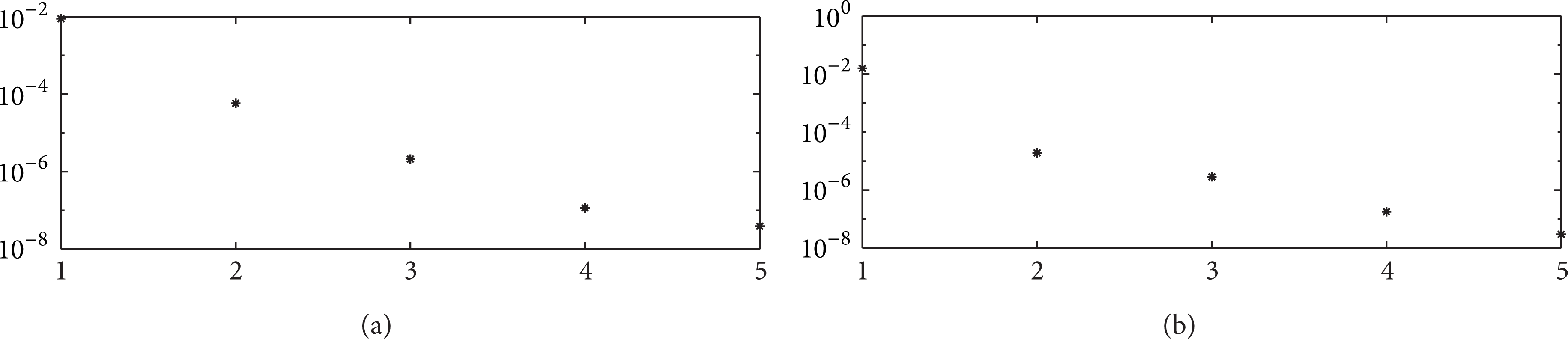
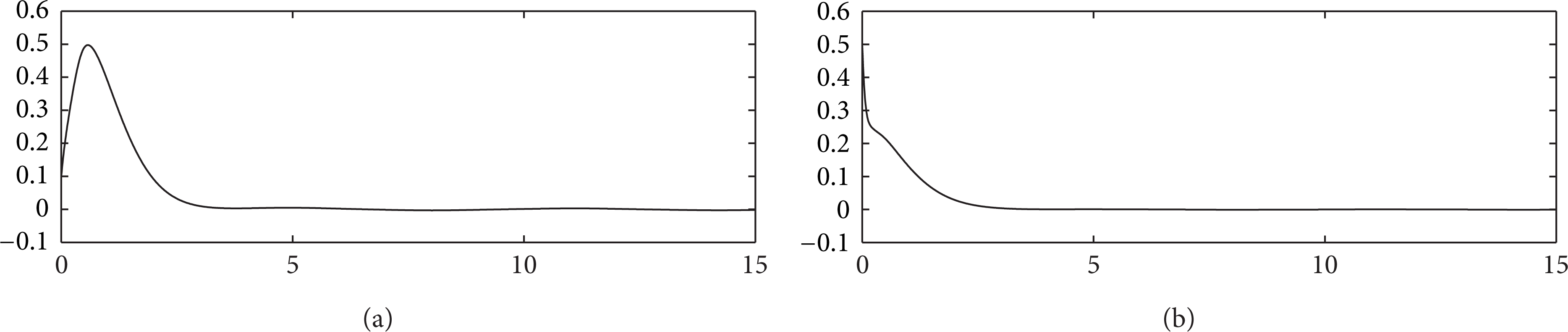
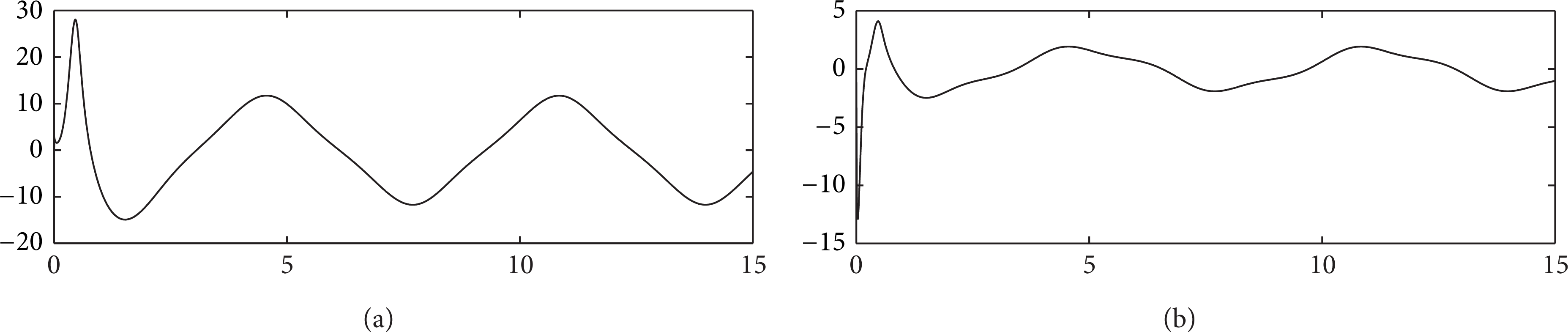
In order to show the robustness to the varying initial output tracking error, we first assume the initial joint position vector of the two-link planar robotic system taking the following arbitrary values for the first five iterations: q ^j (0) = [q₁ ^j (0),q₂ ^j (0)]^⊤ = [0.05, 0.3]^⊤,[0.25, 0.8]^⊤,[0.14, 0.6]^⊤,[0.09, 0.4]^⊤,[−0.1, 0.5]^⊤. At the beginning of each iteration, the initial value of the boundary layer ϕ ^j (t) is then chosen according to ${\varphi }^j(\mathrm{0})={\varepsilon }^j=\left|{[e_{a,\mathrm{1}}^j(\mathrm{0}),e_{a,\mathrm{2}}^j(\mathrm{0})]}^{\top }\right|=\left|{[{\tilde{e}}_{\mathrm{1}}^j(\mathrm{0}),{\tilde{e}}_{\mathrm{2}}^j(\mathrm{0})]}^{\top }\right|=\left|{[e_{\mathrm{1}}^j(\mathrm{0}),e_{\mathrm{2}}^j(\mathrm{0})]}^{\top }\right|=\left|{[\sin (\mathrm{0})\hspace{0.17em}-\hspace{0.17em}{q}_{\mathrm{1}}^j(\mathrm{0}),\cos (\mathrm{0})-q_{\mathrm{2}}^j(\mathrm{0})]}^{\top }\right|$ . For example, ϕ¹(0) = 0.05,ϕ²(0) = 0.25,ϕ³(0) = 0.14,ϕ⁴(0) = 0.09, and ϕ⁵(0) = 0.1. To study the effect of learning performances, ${\sup }_{t\in [\mathrm{0,15}]}|e_{\varphi ,\mathrm{1}}^j(t)|$ and ${\sup }_{t\in [\mathrm{0,15}]}|e_{\varphi ,\mathrm{2}}^j(t)|$ versus iteration j are shown in Figures 1(a) and 1(b), respectively. It is clear that the asymptotic convergence proved in (T1) of Theorem 4 is achieved. Since the learning process is almost completed at the 5th iteration, we demonstrate the auxiliary errors e_{a, 1}⁵(t) and e_{a, 2}⁵(t) in Figures 2(a) and 2(b), respectively. The trajectories of e_{a, 1}⁵(t) and e_{a, 2}⁵(t) satisfy −0.5e^–10t ≤ e_{a, 1}⁵(t) ≤ 0.5e^–10t and −0.5e^–10t ≤ e_{a, 2}⁵(t) ≤ 0.5e^–10t, respectively. This clearly proves (T2) of Theorem 4. The output tracking errors e₁⁵(t) and e₂⁵(t) are shown in Figures 3(a) and 3(b) with satisfied performance even there exists varying initial output errors. The nice tracking performances at the 5th iteration between joint position vector q ^j (t) = [q₁ ^j (t),q₂ ^j (t)]^⊤ and desired joint position vector q _d (t) = [q_{d, 1}(t),q_{d, 2}(t)]^⊤ are presented in Figures 4(a) and 4(b), respectively. Finally, the bounded learned control forces u₁⁵(t) and u₂⁵(t) are plotted in Figures 5(a) and 5(b), respectively.

Figure 1:

(a) ${\sup }_{t\in [\mathrm{0,15}]}\left|e_{\varphi ,\mathrm{1}}^j(t)\right|$ versus iteration j; (b) ${\sup }_{t\in [\mathrm{0,15}]}\left|e_{\varphi ,\mathrm{2}}^j(t)\right|$ versus iteration j.

Figure 2:

(a) e_{a, 1}⁵(t) (solid line) and ± ϕ⁵(t) (dotted lines) versus time t; (b) e_{a, 2}⁵(t) (solid line) and ± ϕ⁵(t) (dotted lines) versus time t.

Figure 3:

(a) e₁⁵(t) versus time t; (b) e₂⁵(t) versus time t.

Figure 4:

(a) q₁⁵(t) (solid line) and q_{d, 1}(t) (dotted line) versus time t; (b) q₂⁵(t) (solid line) and q_{d, 2}(t) (dotted line) versus time t.

Figure 5:

(a) u₁⁵(t) versus time t; (b) u₂⁵(t) versus time t.

6. Conclusion

An observer-based adaptive filtered-FNN iterative learning controller for repeated tracking control of uncertain robotic systems is proposed in this paper. A tracking error observer is designed to estimate the unknown joint variables since only joint positions are assumed to be measurable. An error observation dynamic based on the tracking error observer is derived for the design of the iterative learning controller. The main control force is designed by using a technique of averaging filter and some auxiliary signals. In this main control force, a fuzzy neural learning component based on a filtered-FNN is used to approximate the unknown nonlinear function, a robust learning component is designed to compensate for the other uncertainties, and a stabilization term is applied to guarantee the boundedness of internal signals. The adaptive laws combining time domain and iteration domain adaptation for the network parameters and control parameters are proposed to ensure the stability and convergence of the learning system. A Lyapunov-like analysis has been developed to solve both boundedness of internal signals inside the closed-loop system and asymptotic convergence of learning error. It is shown that the output tracking error asymptotically converges to a tunable residual set whose level of magnitude can be tuned by design parameters as the iteration number increases.