Sage Journals: Discover world-class research

Abstract

A major problem associated with the membrane separation processes is the permeate flux drop, limiting the widespread of industrial application of this process. This occurs due to the accumulation of solute concentration near the membrane surface. An exact quantification of the concentration polarization as a function of process conditions is essential to estimate the system performance satisfactorily. In this sense, this work aims to predict the behavior of the concentration polarization boundary layer along the length of a permeable tubular membrane, over various operation conditions. The numerical solution of the Navier-Stokes equation, coupled to Darcy's and mass transfer equations, is obtained by the commercial software ANSYS CFX 12, considering a two-dimensional computational domain. The study evaluates the effects of axial Reynolds and Schmidt numbers on the concentration polarization boundary layer thickness during the cross-flow filtration process. Numerical results have shown that the mathematical model is able to predict the formation and growth of the concentration polarization boundary layer along the length of the tubular membrane.

1. Introduction

In the manufacturing industry, in order to get the final product with the desired specifications, it is essential to separate, concentrate, and purify the chemical species present in the different streams resulting from these transformations. The membrane separation processes (MSP) have been frequently used in the separation stages of industrial processes. Presently, the membrane technology area unfolds in a wide variety of applications and requires a multidisciplinary approach. Its wide application led to the development of many theories to describe the mass transport during the separation process.

One of the main topics related to rate of growth of the concentration polarization boundary layer of a solute on the membrane surface has been reported by several studies [1 –3]. According to these authors, the concentration polarization is a reversible phenomenon that starts in the first minutes of filtration and consists in the formation of a concentration profile perpendicular to the membrane surface, resulting in an increase in the retained species concentration near the membrane surface. The establishment of a concentration gradient in the boundary layer causes an additional resistance to mass transfer, which leads to a decrease in the permeate flow.

Paris et al. [4] report a theoretical study about the phenomenon of concentration polarization in ultrafiltration membranes. The authors have proposed a two-dimensional model based on diffusion and convection equations, coupled with a modified model of series resistance, in order to include the influence of the average solute concentration and transmembrane pressure on the flow resistance due to concentration polarization along the membrane length. According to the authors, at higher initial concentrations (>8 g/L), predicted permeate flux showed good agreement with the experimental results. However, at low initial concentration (1 g/L), the results were not satisfactory.

According to Damak et al. [5 –7] and Pak et al. [8], as the fluid is forced to pass under the membrane in crossflow, the solvent is forced to flow through the membrane due to the action of a pressure difference across the permeable membrane. The decrease in permeate flow rate is closely related to the decrease in driving force and increased resistance to permeation. Particles present in the inlet stream are conducted by convection to the membrane surface and finally accumulate near the membrane surface, until the balance between the convective and diffusive flow is reached. Using the gel layer model, Paris et al. [4] found that the gel layer thickness increases with pressure, and the membrane surface concentration is dependent on the inlet velocity. According to the work of several researchers such as Kulkarni et al. [9], Zaini et al. [10], and Abadi et al. [11] there is the wide use of membranes in various application fields focusing on reducing fouling and polarized layer, thus increasing the permeate flux through chemical, physical, and hydrodynamic methods. Vieira et al. [12] studied the oil/water separation process by tangential microfiltration. The authors found that changes in the inlet flow rate, as well as the geometry of the tubular membrane module, providing a swirling flow, can optimize the separation process, thus increasing the permeate volume. Souza [13] evaluated the effect of physical and geometrical parameters of the flow on the behavior of the three-dimensional polarized boundary layer. The author observed that the size, structure, and development of the polarized boundary layer around the membrane vary greatly with angular direction, with reductions in the annular space and shape of the inlet and outlet of the ducts.

From the review cited before, the great problem in the membrane as device to filtration is related to decline in permeate flux crossing the membrane due to concentration polarization phenomena. In this sense, this work aims to study the concentration polarization phenomenon on the surface of a permeable tubular membrane and investigate the effect of several physical parameters on the concentration profiles along the membrane surface.

2. Methodology

2.1. Problem Description

The physical problem consists of a tangential flow of a fluid inside a tubular membrane with an effluent inlet and a concentrated outlet. The filtrate is collected through the external porous membrane wall, as shown in Figure 1.

Figure 1:

Scheme of the tubular membrane and direction of the fluid flow.

Due to the axial symmetry in the tubular membrane, a cross-section was taken in the plane (r, z) of this device, as illustrated in Figure 2. In this figure, one may notice that the domain used in this work is composed only of the fluid region, not covering the membrane. It was assumed that the reduction on the permeate flow occurs only due to concentration polarization.

Figure 2:

Transverse plane detail selected for the 2D numerical study.

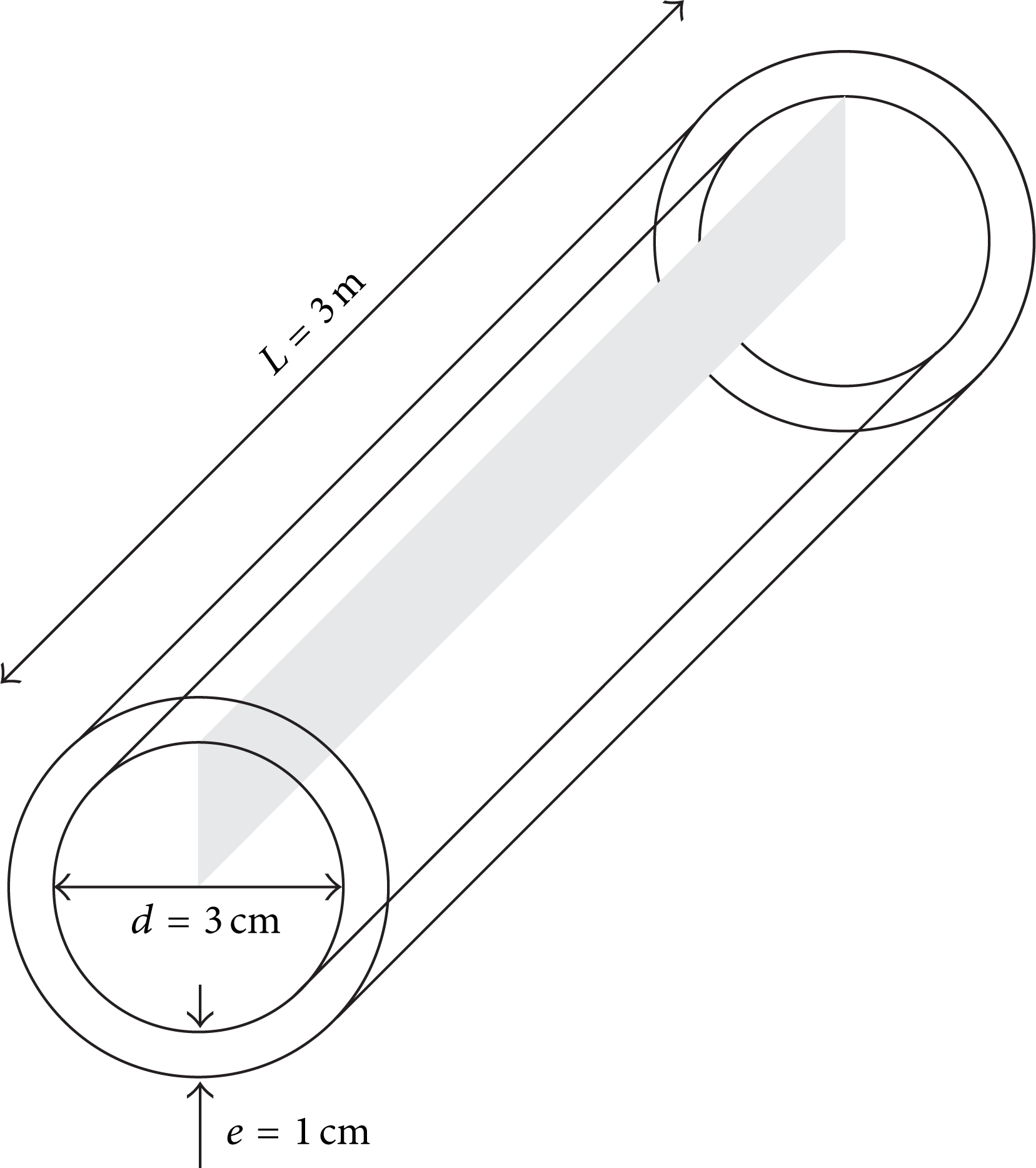
The membrane has dimensions of 3 m length (L), 3 cm inner diameter (d_i), and 1.0 cm thickness (e). The two-dimensional domain adopted for the numerical study has a length equal to the membrane, 3 m, and radius, 1.5 cm, as seen in Figure 3.

Figure 3:

Dimensions of the two-dimensional domain used in this work.

2.2. Mathematical Model

Mathematical modeling is a physical representation of reality in the form of a set of consistent equations. The tubular membrane has been assumed to be operating at steady state conditions, where the classical equations of fluid dynamics can be applied. So, the continuity, momentum, and concentration equations were used to determine the concentration profiles and concentration boundary layer thickness. This work deals with the mass transfer phenomenon in a tubular membrane (r, z) with radius R and length L (Figure 3). The analysis is based on the following assumptions:

the flow is laminar;

the solute diffusion coefficient is considered constant;

because of the low concentration of contaminant, the fluid viscosity and fluid density are constant and equal to the pure solvent;

the fluid is incompressible and the steady state conditions are controlled;

there is no gravity effect;

the fluid movement is considered symmetrical around the z-axis; therefore just a section of the tube is considered;

the wall permeation velocity is determined from the series resistance model;

the concentration layer on the surface of the porous membrane is considered homogeneous.

The geometric structure of the tubular membrane has an axial symmetry; therefore, the study is performed in the plane (r, z). Taking these assumptions into account, the two-dimensional mathematical model used to describe the flow inside the tubular membrane corresponds to the following equations.

Mass conservation equation:

\frac{1}{r} \frac{\partial U_{r}}{\partial r} + \frac{\partial U_{z}}{\partial z} = 0 .

(1)

Momentum conservation equation:

\begin{matrix} \frac{\partial U_{z}}{\partial t} + ρ (U_{r} \frac{\partial U_{z}}{\partial r} + U_{z} \frac{\partial U_{z}}{\partial z}) = - \frac{\partial P}{\partial r} + μ [\frac{1}{r} \frac{\partial}{\partial r} (r \frac{\partial U_{z}}{\partial r}) + \frac{\partial^{2} U_{z}}{\partial z^{2}}] . \end{matrix}

(2)

Mass transport equation:

\vec{U} \cdot \nabla C = D \nabla^{2} C .

(3)

In the extended form, (3) will be written as follows:

U_{r} \frac{\partial C}{\partial r} + U_{z} (\frac{\partial C}{\partial z}) = D (\frac{1}{r} \frac{\partial}{\partial r} (r \frac{\partial C}{\partial r}) + \frac{\partial^{2} C}{\partial z^{2}}) .

(4)

2.3. Boundary Conditions

The elliptic nature of the mass transport equation requires the specification of the boundary conditions for velocity and solute concentration, such as that represented in Figure 4. In this work, the following boundary conditions were used.

Figure 4:

Representation of the membrane boundaries.

(a) At the Porous Tube Input (z = 0). It is assumed that the flow is hydrodynamically established at the inlet of the porous tube. Therefore, the axial velocity profile at the inlet is identical to Poiseuille parabolic profile and the radial component of velocity is zero:

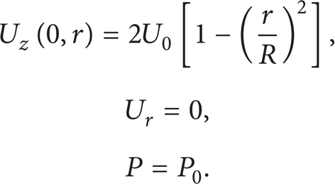
\begin{matrix} U_{z} (0, r) = 2 U_{0} [1 - {(\frac{r}{R})}^{2}], \\ U_{r} = 0, \\ P = P_{0} . \end{matrix}

(5)

The liquid is fed into the tube at an initial prescribed contaminant concentration:

C = C_{0} .

(6)

(b) At the Tube Outlet (Concentrate, z = L). The boundary condition downstream the tube was assumed to be equal to atmospheric pressure (P = 1 atm).

(c) In the Center of the Tube (r = 0). The boundary conditions on the tube axis are symmetry conditions. Thus, we can write

\begin{matrix} \frac{\partial U_{z}}{\partial r} = 0, \\ \frac{\partial U_{r}}{\partial r} = 0, \\ \frac{\partial C}{\partial r} = 0 . \end{matrix}

(7)

(d) In the Porous Tube Wall (Permeate, r = R). At the membrane wall, no-slip boundary condition is assumed, that is, the axial component of velocity in the wall equal to zero, regardless of the local roughness influence, due to the porous nature of the wall:

U_{z} = 0 .

(8)

In the porous wall, the radial component of velocity is equal to the permeation velocity:

U_{r} = U_{w} .

(9)

The diffusive flux in the polarized layer (concentration polarization layer) is described by the mass transport equation, (10), which is added to the model as a source term. Thus,

U_{w} C = D \frac{\partial C}{\partial r} .

(10)

The local permeation velocity is given by Darcy's law, written as the resistance-in-series model [4 –8]:

U_{w} = \frac{Δ P}{μ (R_{m} + R_{p})},

(11)

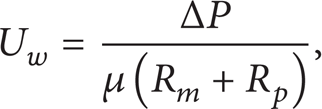
where ΔP, R_m, and R_p are, respectively, the transmembrane pressure, membrane hydraulic resistance, and the specific resistance of concentration polarization layer.

If the fluid is laden with particulates, the membrane is obstructed. Herein, it was assumed that the blocking is due to the concentration layer formation. The specific resistance due to the concentration polarization is a very important parameter that affects the permeate flux.

According to the frontal filtration (dead-end filtration), the specific resistance of concentration polarization layer is defined as the resistance per unit of concentration polarization thickness:

R_{p} = \int_{R - δ_{c}}^{R} r_{p} d δ,

(12)

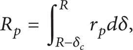
where r_p is the specific resistance and δ is the concentration polarization layer thickness.

Assuming that the concentration in the boundary layer is homogeneous, (12) takes the form

R_{p} = r_{p} δ_{c} .

(13)

The equation used to determine the thickness of the local concentration boundary layer was developed by Damak et al. [6]. In this equation, the concentration boundary layer thickness, δ_c, is approximately equal to the distance between the membrane surface and a value where the concentration is sufficiently close to the inlet concentration, so that the balance between the convective and diffusive flows is achieved when $(C - C_{0}) / C_{0} < 0.001$ . According to [6], δ_c can be described by the following equation:

δ_{c} = 2 d {(\frac{z}{d})}^{0.33} {(ReSc)}^{- 0.33} {Re}_{w}^{- 0.3} \times (1 - 0.4377 {Sc}^{- 0.0018} {Re}_{w}^{- 0.1551}),

(14)

where d is the inner diameter of the tubular membrane, z represents the axial coordinate along the membrane, $Re = ρ {\bar{U}}_{o} d / μ$ is the axial Reynolds number, Re_w is the wall Reynolds number $R e_{w} = ρ {\bar{U}}_{w o} d / μ$ , and Sc = μ/ρD is the Schmidt number. The conditions of use of correlation (14) are such that Sc = 600∼3200, Re = 300∼1000, Re_w = 0.02∼0.3, and z/d = 0∼100. According to [6], these parameters correspond to a separation membrane system for the liquid ultrafiltration, with low particles concentration and laminar flow in the porous tube wall.

The specific resistance r_p can be determined by Carman-Kozeny correlation as follows:

r_{p} = 180 \frac{{(1 - ε_{p})}^{2}}{a_{p}^{2} ε_{p}^{2}},

(15)

where a_p is the average solute particle diameter and ε_p is the porosity of the concentration polarization layer. Equation (15) is available for dispersed nondeformable spherical particles and porosity 0.35 ≤ ε_p ≤ 0.75.

Figure 5 illustrates the concentration boundary layer which is formed on the surface of the porous membrane.

Figure 5:

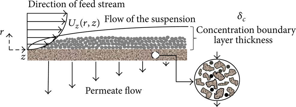
Schematic representation of the concentration boundary layer.

2.4. Fluid Properties and Geometrical Data Used in the Simulations

Other important data that were defined in the problem solution are those related to the fluid properties and the media in which it is flowing. These properties are listed in Table 1.

Table 1:

Physical and chemical properties of the fluids and the membrane.

Contaminant	Droplet diameter	63 µm	Damak et al. [6]
Contaminant	Inlet concentration	1000 ppm	Damak et al. [6]

Water	Dynamic viscosity	50 cP	Damak et al. [6]
	Molar mass	18.02 kg/kmol	Ansys CFX
	Density	997 kg/m³	Ansys CFX

Membrane	Porosity	0.35	Damak et al. [6]
Membrane	Permeability	1 × 10⁻⁸ m²	Damak et al. [6]

2.5. Numerical Procedure

In this work the ANSYS CFX software was used to solve the governing equations: the ANSYS CFX software uses the following general form of the transport equation for a potential variable:

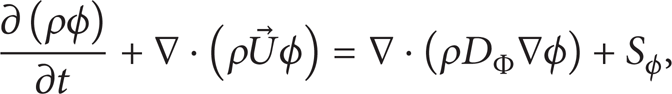
\frac{\partial (ρ ϕ)}{\partial t} + \nabla \cdot (ρ \vec{U} ϕ) = \nabla \cdot (ρ D_{Φ} \nabla ϕ) + S_{ϕ},

(16)

where ρ is the mixture density, mass per volume unit, Φ is the conserved quantity per volume unit or concentration, ϕ = Φ/ρ is the conserved quantity per mass unit, S_ϕ is a volumetric source term, with units of conserved quantity per volume unit per time unit, and D_Φ is the kinematic diffusivity.

A representative mesh of the porous membrane was generated according to [6]. The resulting mesh is shown in Figure 6. The representative mesh has 77961 elements and 160000 nodes. From the analysis of the mesh we can observe a higher density of elements in the inlet region and near the interface region between the fluid and the porous medium. This refinement is of fundamental importance in the numerical study, considering that, in the membrane inner wall, the formation of the concentration boundary layer (concentration polarization) occurs, which has low thickness, justifying a greater concern with the mesh in this region.

Figure 6:

Mesh generated for the two-dimensional domain (a) and detail of the mesh (b).

3. Results and Discussions

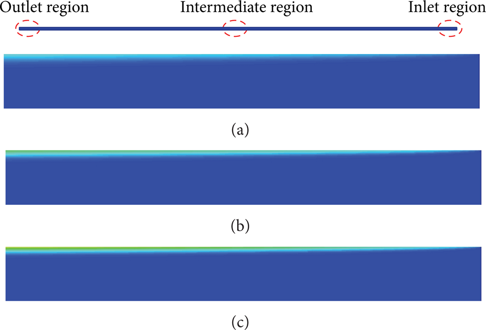
The analysis of the concentration profiles plays important role in microfiltration cross-flow membrane design. In this work, the concentration profiles and concentration boundary layer thickness are presented and analyzed for Reynolds numbers 300, 600, and 1000 and Schmidt numbers 1000, 2000, and 3000 (see Figures 7 –17). An analysis of the cited figures shows that there are concentration variations in the region near the porous membrane wall in all of the analyzed cases. This behavior is due to fact that the particles are transported by convection to the membrane surface, where they accumulate. Thus, a very thin polarization layer appears, in which the concentration variation is located.

Figure 7:

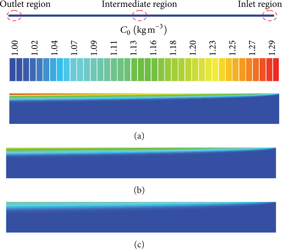
Concentration boundary layer thickness and contaminant concentration in the entrance region of the membrane (Sc = 1000). (a) Re = 1000, (b) Re = 600, and (c) Re = 300.

Figures 7, 8, and 9 show the concentration profiles in the entrance and exit region of the membrane for the variation of Reynolds numbers of 300, 600, and 1000. These results showed that an increase in Reynolds number causes both decreases in the concentration polarization layer thickness and an increase in the fluid concentration near the region of the fluid-membrane interface and along the membrane length. Thus, an increase in inlet axial velocity can improve the separation performance of the tubular membrane. Further, we can see that a large region appears where the concentrations are constant.

Figure 8:

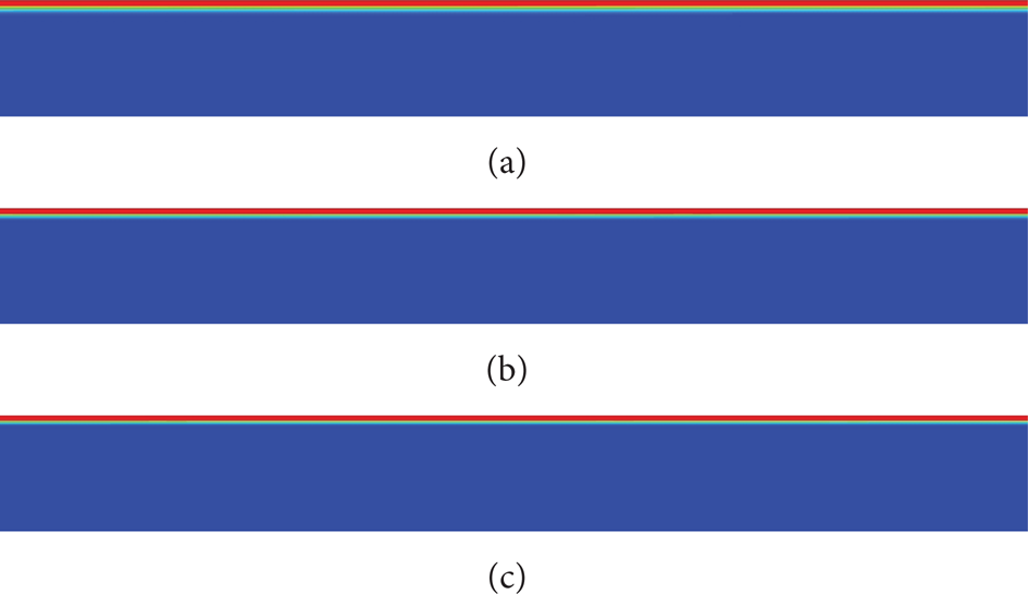
Concentration boundary layer thickness and contaminant concentration in an intermediate region of the membrane (Sc = 1000). (a) Re = 1000, (b) Re = 600, and (c) Re = 300.

Figure 9:

Concentration boundary layer thickness and contaminant concentration in the outlet region of the membrane (Sc = 1000). (a) Re = 1000, (b) Re = 600, and (c) Re = 300.

Figure 10 shows the behavior of the dimensionless concentration polarization layer thickness as a function of the dimensionless axial distance for different Reynolds number. Through the analysis of the figure, we can verify that an increase in the Reynolds number causes an increase of the shear stress, which results in a smaller concentration boundary layer thickness. These results are in agreement with results obtained by Damak et al. [7] and Pak et al. [8]. Further, the growth rate of concentration boundary layer is almost constant as z/d>70.

Figure 10:

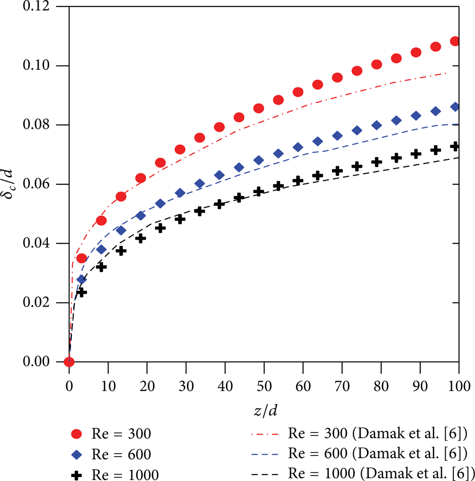
Boundary layer concentration thickness along the membrane (Sc = 1000 and Re_w = 0.1).

The increase in axial Reynolds number (Re) induced a raise in the permeate rate as illustrated in Figure 11, due to the decreasing concentration boundary layer and an increase in wall filtration velocity [8, 14]. The particles are moved by convection to the membrane surface under the transmembrane pressure effect, causing an increase in the concentration in the membrane-fluid interface. However, this result was contrary to that obtained by Damak et al. [6] as illustrated in Figure 12. The difference between the results is probably due to the fact that Damak et al. [6] used a velocity profile for all domains and neglected the radial pressure drop. Another explanation for this difference can be attributed to the coupling between the momentum and the mass equations. Damak et al. [6] have realized numerical solution with uncoupling equation. In the present research, this coupling was applied. Figures 13, 14, and 15 show the concentration profiles at the inlet, intermediate, and outlet regions of the membrane for different Schmidt numbers. It can be seen that increasing the Schmidt number reduces the tendency of the particles back diffusing into the feed stream due to the decrease in the diffusion coefficient and provokes a reduction in the concentration boundary layer thickness. Furthermore, the concentration profile changes dramatically as a function of the Schmidt number, so, more particles are expected to accumulate close to the membrane surface, thus, increasing the contaminant concentration in this region. These numerical results are in agreement with literature [6, 8, 13].

Figure 11:

Permeate velocity as a function of the average transmembrane pressure (Sc = 1000 and Re_w = 0.1).

Figure 12:

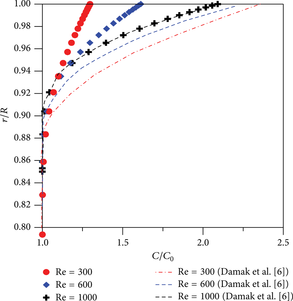
Reynolds number effect in the radial concentration profile (z/d = 50, Sc = 1000, and Re_w = 0.1).

Figure 13:

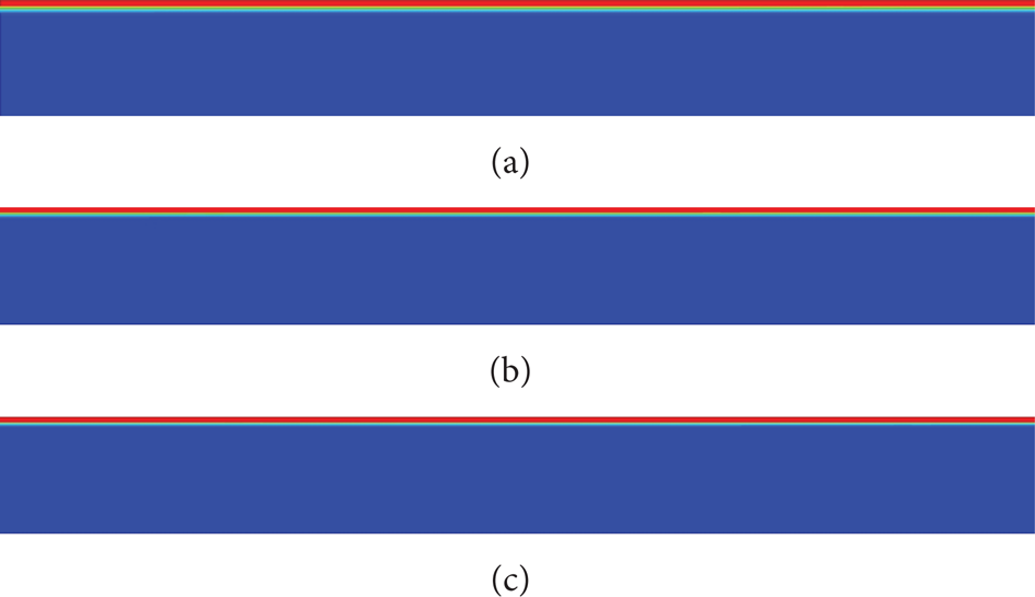
Concentration boundary layer thickness and contaminant concentration in the entrance region of the membrane (Re = 1000 and Re_w = 0.1). (a) Sc = 1000, (b) Sc = 2000, and (c) Sc = 3000.

Figure 14:

Concentration boundary layer thickness and contaminant concentration in an intermediate region of the membrane (Re = 1000 and Re_w = 0.1). (a) Sc = 1000, (b) Sc = 2000, and (c) Sc = 3000.

Figure 15:

Concentration boundary layer thickness and contaminant concentration in outlet region of the membrane (Re = 1000 and Re_w = 0.1). (a) Sc = 1000, (b) Sc = 2000, and (c) Sc = 3000.

Figure 16 illustrates the behavior of the local concentration boundary layer thickness along the axial distance. From the analysis of this figure, it was possible to observe, quantitatively, that increasing the Schmidt number causes a reduction in the diffusion coefficient, thus increasing the contaminant concentration in the interface with the porous membrane wall (Figure 17) and consequently decreasing the thickness of the concentration boundary layer from 0.073 to 0.051. We can see in Figure 17 that dimensionless concentration profiles change strongly as a function of the Schmidt number. In this work, laminar flow was established. However according to Pak et al. [8] and Vieira et al. [12], turbulent condition can improve the separation performance of the membrane. This behavior is consistent with that reported by Damak et al. [5, 6].

Figure 16:

Concentration boundary layer thickness as a function of the dimensionless axial distance (Re = 1000 and Re_w = 0.1).

Figure 17:

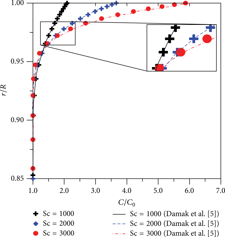
Schmidt number effect in the concentration profile (z/d = 50, Re = 1000, and Re_w = 0.1).

4. Conclusions

In this paper, diffusion-convection phenomena in tubular membrane have been explored. Emphasis is given to ultrafiltration process and polarization concentration boundary layer. Interest in this type of problem is motivated by its importance in many practical situations related to fluid treatment. The numerical study has been done by using the ANSYS CFX software. From the predicted results reported in this paper we can conclude the following.

The mathematical model used predicts with success the fundamental mechanisms involved in the behavior of the losses in the permeate flux during cross-flow filtration, emphasizing the influence of the membrane length in the axial concentration profiles.

An increase in the axial Reynolds number leads to a decrease in the thickness of the concentration boundary layer. For higher Schmidt numbers we have a decrease in the local concentration boundary layer thickness.

The increased axial Reynolds number leads to an increase of the system pressure, thereby causing an increase in the transmembrane pressure, which results in a higher solute concentration on the membrane surface.

Conflict of Interests

The authors declare that there is no conflict of interests regarding the publication of this paper.

Footnotes

Acknowledgments

The authors would like to express their gratitude to the Brazilian research agencies CNPq, CAPES, FINEP, ANP, and PETROBRAS for supporting this work and to the authors of the references cited in the paper, who helped to improve its quality.

References

Baker

R. W.

, Membrane Technology and Applications, John Wiley & Sons, New York, NY, USA, 2nd edition, 2004.

Lautenschlager

S. R.

Filho

S. S. F.

, and Pereira

, “Mathematical modeling and operational optimization of ultrafiltration membrane processes,” Sanitary Engineering and Environmental, vol. 14, no. 2, pp. 215–222, 2009 (Portuguese).

Song

, “Flux decline in crossflow microfiltration and ultrafiltration: mechanisms and modeling of membrane fouling,” Journal of Membrane Science, vol. 139, no. 2, pp. 183–200, 1998.

Paris

Guichardon

, and Charbit

, “Transport phenomena in ultrafiltration: a new two-dimensional model compared with classical models,” Journal of Membrane Science, vol. 207, no. 1, pp. 43–58, 2002.

Damak

Ayadi

Schmitz

, and Zeghmati

, “Modeling of crossflow membrane separation processes under laminar flow conditions in tubular membrane,” Desalination, vol. 168, no. 1–3, pp. 231–239, 2004.

Damak

Ayadi

Zeghmati

, and Schmitz

, “Concentration polarisation in tubular membranes—a numerical approach,” Desalination, vol. 171, no. 2, pp. 139–153, 2005.

Damak

Ayadi

Zeghmati

, and Schmitz

, “A new Navier-Stokes and Darcy's law combined model for fluid flow in crossflow filtration tubular membranes,” Desalination, vol. 161, no. 1, pp. 67–77, 2004.

Pak

Mohammadi

Hosseinalipour

S. M.

, and Allahdini

, “CFD modeling of porous membranes,” Desalination, vol. 222, no. 1–3, pp. 482–488, 2008.

Kulkarni

S. S.

Funk

E. W.

, and Li

N. N.

, “Ultrafiltration,” in Membrane Handbook, Winston Ho

W. S.

and Sirkar

K. K.

, Eds., chapter 8, Van Nostrand Reinhold, New York, NY, USA, 1992.

10.

Zaini

M. A. A.

Holdich

R. G.

, and Cumming

I. W.

, “Crossflow microfiltration of oil in water emulsion via tubular filters: evaluation by mathematical models on droplet deformation and filtration,” Jurnal Teknologi, vol. 53, pp. 19–28, 2010.

11.

Abadi

S. R. H.

Sebzari

M. R.

Hemati

Rekabdar

, and Mohammadi

, “Ceramic membrane performance in microfiltration of oily wastewater,” Desalination, vol. 265, no. 1–3, pp. 222–228, 2011.

12.

Vieira

T. M.

Souza

J. S.

Barbosa

E. S.

Cunha

A. L.

Farias Neto

S. R.

, and Lima

A. G. B.

, “Numerical study of oil/water separation by ceramic membranes in the presence of turbulent flow,” Advances in Chemical Engineering and Science, vol. 2, no. 2, pp. 257–265, 2012.

13.

Souza

J. S.

, Theoretical study of the microfiltration process in ceramic membranes [Ph.D. thesis], Process Engineering, Federal University of Campina Grande, Campina Grande, Brazil, 2014, (Portuguese).

14.

Geraldes

Semião

, and Pinho

M. N.

, “Flow and mass transfer modelling of nanofiltration,” Journal of Membrane Science, vol. 191, no. 1–2, pp. 109–128, 2001.

Separation Process by Porous Membranes: A Numerical Investigation

Abstract

1. Introduction

2. Methodology

2.1. Problem Description

2.2. Mathematical Model

2.3. Boundary Conditions

2.4. Fluid Properties and Geometrical Data Used in the Simulations

2.5. Numerical Procedure

3. Results and Discussions

4. Conclusions

Conflict of Interests

Footnotes

Acknowledgments

References