Modeling Flexible Bodies in Multibody Systems in Joint-Coordinates Formulation Using Spatial Algebra

Abstract

This paper presents an efficient approach of using spatial algebra operator to formulate the kinematic and dynamic equations for developing capabilities to model flexible bodies within general purpose multibody dynamics solver. The proposed approach utilizes the joint coordinates and modal elastic coordinates as the system generalized coordinates. The recursive nonlinear equations of motion are initially formulated using the Cartesian body coordinates (CBC) and the joint coordinates (JC) to form an augmented set of differential algebraic equations. The system connectivity matrix is derived from system topological relations and is used to project the Cartesian quantities into the joint subspace leading to minimum set of differential equations. The modal transformation matrix is used to describe the finite element kinematics in terms of a small set of generalized modal coordinates. Although the resulting stiffness matrix is constant, the mass matrix depends on the generalized elastic modal coordinates and needs to be updated at each time step. To reduce the computational efforts, a set of precomputed inertia shape invariants (ISI) can be identified and used to update the flexible body mass matrix. In this proposed joint-coordinates formulation, the transformation operations required for the flexible body inertia matrix are different from those in case of CBC formulation. The necessary ISI and the algorithm to reconstruct the modal mass matrix will be presented in this paper.

1. Introduction

Virtual development procedures became the most economical venue in product design and optimization. Modeling and simulation of the elastic components in multibody systems became an integral part of the virtual product simulation. During operation, flexible components and light-structure are prone to excessive vibration. The vibration could be excited by driving over rough road or terrain, internally moving components like engines, or due to work cycle loads excitations. Structural components and light fabrications (LF) are subject to static and fatigue failure. Cyclic elastic deformation of the flexible structures due to vibration can initiate crack propagation leading to structural failure. Also, high frequency elastic deformation can generate severe structural noise leading to unacceptable noise levels. Accurate prediction of the flexible body's transient response to the applied loads and accuracy in predicting the loads become essential requirements to insure that the design will have adequate fatigue durability. Although LF and structural components can be modeled using the same technique, the nature of loading and response may require different considerations for simulating LF.

Designers usually recommend using robust and accurate analytical tools in performing transient analysis to accurately predict the loads and excitations and compute the resulting stresses and strains in the flexible body. Then the fatigue life of the component could be utilized as the acceptance criteria for the flexible body design. Such simulations should be able to capture law as well as high frequency excitations that may excite the high frequency resonance of the flexible body. As a result of including the high frequency excitations, the integrator time step should be small enough to capture those high frequency excitations and the resulting response. As the integrator time step decreases and the number of DoF increases, the simulation time increases significantly calling for more computing resources. This requires efficient multibody simulation algorithms that can model flexible bodies while maintaining minimum number of DoF.

Three traditional approaches have been used to formulate the multibody equations: the Cartesian body coordinates (absolute coordinates), the joint coordinates, and velocity transformation method. The Cartesian body coordinates formulations are very popular and reported to be a simpler method to construct the equations of motion leading to a large set of differential-algebraic equations [1, 2]. The configuration of a rigid body is described by a set of translational and rotational coordinates. Algebraic constraints are introduced to represent kinematic joints connecting bodies and then the Lagrange multiplier technique is used to describe joint reaction forces. The system of differential-algebraic equations has to be solved simultaneously. Newton-Raphson iterations or similar techniques could be used to satisfy the applied constraints. Although these formulations are easy to construct, one of the main drawbacks is that their computational inefficiency especially simulating systems with large number of degrees of freedom and with high frequency contents leads to very long simulation time. Implementing the flexible body dynamics in CBC formulation has been demonstrated by many researchers and has been used in many commercial software packages [3–6]. Nikravesh [2, 7] presented an overview of the difference between body coordinate formulations based on Newton-Euler equations of motion and the joint based coordinated formulations. In this paper, Nikravesh presented using the velocity relations to transform one formulation to the other. Appending the deformable body into the multibody system was also discussed.

Featherstone [8–10] used spatial vectors to study the dynamics of articulated bodies. Featherstone and Orin [11] and Featherstone [12] presented an efficient approach for utilizing spatial algebra to model multibody systems and efficiently factor the inertia matrix for rigid body systems. Wehage and Haug [13] used a similar approach to develop a set of automated procedures for robust and efficient solution of over-constrained multibody dynamics. Wehage and Belczynski [14] proposed structuring the kinematic and dynamic equations into block-matrix structure and developed procedures to enable real-time simulation of multibody system. Rodriguez et al. [15, 16] presented a spatial operator based on the spatial algebra for developing multibody dynamic equations of motion.

The flexible body dynamics were implemented in joint-coordinates based formulations [17]. Newton-Euler factorization of the mass matrix leads to recursive algorithm for inverse dynamics and composite-body forward dynamics. Nikravesh [18] presented semiabstract form for the equations of motion of rigid and flexible body, where he focused on the reduction techniques. The different methods to attach a body frame to a moving deformable body and the model reduction techniques were reviewed. Also the advantages and disadvantages of each technique were briefly discussed. Mukherjee and Anderson [19] presented an efficient implementation of the parallel processing of multibody systems that include flexible bodies. Although many researchers have implemented flexible body capabilities in joint-coordinates based multibody system, some of these implementation did not account for the changes of flexible body inertia matrix due to deformation. Other formulations did not show details of the implemented inertia shape invariants. A primary contribution of this paper will be detailing the inertia shape invariants for the flexible body in joint-coordinates based formulation using spatial algebra.

This paper describes a general purpose formulation and implementation for modeling flexible body in multibody system based on the joint-coordinates formulation. The presented approach utilizes a recursive scheme to evaluate the equations of motion. The spatial algebra operators are used to formulate the kinematic and dynamic equations of motion. This paper is organized as follows. In the following section the structure of the equation of motion of the multibody system using joint-coordinates formulation is introduced. In Section 3, the flexible body kinematic and dynamic equations of motion are presented, and the component mode synthesis approach and inertia shape integrals based on the spatial algebra are presented in detail. In Section 4, the multibody system equations of motion including rigid and modal flexible bodies will be presented. Section 5 provides an outline of the recursive algorithm implemented to solve the proposed multibody system equations of motion. Section 6 discusses some considerations for the pre-/postprocessing operations of the flexible body to be used in the dynamic simulation using the proposed formulation. In Section 8. The following set of conventions will be used: a small letter represents a scalar quantity like mass m, small underlined letter represents a 3D vector with three entries like vector distance $\underset{\_}{t}$ , boldface small letter represents a spatial vector with six elements like spatial velocity v or spatial acceleration a, a capital italic letter with underline represents a 3 × 3 matrix like rotation matrix $\underset{\_}{R}$ , a capital italic letter represents a spatial matrix like 6 × 6 mass matrix M, and a boldface capital letter represents a system level matrix like the assembly influence matrix ${\mathbf{H}}_a^{\ell }$ .

2. Kinematic and Dynamic Equations of Motion of Rigid Body

In the joint-coordinates based formulation, the system is topology described based on the connectivity between the different bodies in the system. Each body is usually connected or referenced to a parent body through an arc joint that allows for one or more DoF. The ground body (the inertial body) is usually considered to be the root of the kinematic tree. While each body can have only one parent (ancestor body), it could have one or more child bodies (descendent bodies). The connectivity graph or the kinematic tree is one way to represent the kinematic relation between the bodies in the system. In the kinematic tree the root body is numbered as 0 while the descendent bodies are numbered consecutively from 1 to n_b. The body and the joint connecting it to its parent are given the same number [3]. Using the parent-child relation, a parent-child list could be developed and stored to be used later in the recursive calculations [12, 20, 21]. Anybody in the system could be modeled as rigid or flexible body.

In the proposed formulation triads or markers will be used very frequently. The triad is composed of three orthogonal unit vectors used to measure relative and absolute motion between different points in the system. The triad position is defined by the position of its origin while the orientation is defined by the rotational matrix. The triad could be referring to a point in the rigid or flexible body. If the body is rigid, the triad position and orientation will remain constant during the dynamic simulation with respect to the body reference frame. If the body is flexible, the triad must be associated with a node in the flexible body. The initial position of the triad is defined with respect to the body reference frame by the node location and the triad orientation could be parallel to the reference frame. During the dynamic simulation, the triad position and orientation may change depending on the elastic deformation at the attachment node.

The child body is joined to its parent through two triads; one triad is attached to the parent side while the other triad is on the child side. The triad in the child side is considered as the output triad and is used as the reference frame of the child body. All the kinematic quantities and dynamic matrices are expressed with respect to the body reference frame. The triad in the parent side is considered as the input triad to the child body, connector triad. The position and orientation of the connectors are measured relative to the parent reference triad through the spatial transformation matrix, as shown in Figure 1.

Figure 1:

Body kinematics and joint connections.

The arc joint DoF or joint variables is defined as the allowed relative motion between the two connecting triads. Relative motion between the triads could be translation or rotation along one of the connector triad axes. Massless triads could be inserted between the two bodies to represent joints with more than one DoF. The joint variables displacement, velocities, and accelerations are used as the body state variables. The Cartesian displacements, velocities, acceleration vectors, and the joint reaction forces are considered as augmented algebraic variables.

The position vector of body i is defined in the global coordinate system by position vector of the origin of the body reference triad of the body ${\underset{\_}{r}}_{\mathrm{0}i,i}^{\mathrm{0}}$ , as shown in Figure 1, while the orientation of the body could be describes by the 3 × 3 rotation matrix ${\underset{\_}{R}}^{\mathrm{0}i}$ as a function of a set of rotational angles. The spatial velocity vector of body i, ${\mathbf{v}}_{\mathrm{0}i,i}^{\mathrm{0}}={\left[\begin{array}{cc}{\underset{\_}{\omega }}_{\mathrm{0}i}^{\mathrm{0}}& {\dot{\underset{\_}{r}}}_{\mathrm{0}i,i}^{\mathrm{0}}\end{array}\right]}^T$ , could be obtained by differentiating the position vector and the orientation parameters. A general spatial velocity vector ${\mathbf{v}}_{ij,k}^i$ is defined in the coordinate system i (designated by the superscript) measuring the velocity difference between two triads i and j (designated by the subscript) and is defined with respect to a certain observer located at k (designated by the subscript after the comma). As the recursive formulation is based on relative motion, the spatial velocity vector of the reference frame of a child body j with respect to its parent rigid body i observed at the origin of the local coordinate system of body j can be written as

${\mathbf{v}}_{ij,j}^j={\left[\begin{array}{cc}{\underset{\_}{\omega }}_{ij}^j& {\dot{\underset{\_}{r}}}_{ij,j}^j\end{array}\right]}^T,$

(1)

where ${\underset{\_}{\omega }}_{ij}^j$ is the time derivative of the orientation parameters of body j with respect to body i and ${\underset{\_}{\dot{r}}}_{ij,j}^j$ is the derivative of the position vector of body j with respect to body i. The spatial velocity vector can be transformed from the CS at j into the CS at i using spatial transformation matrix as follows [2, 7, 8]:

${\mathbf{v}}^i={{}^{m}X}_{ij}^{ij}{\mathbf{v}}^j,$

(2)

where ${{}^{m}X}_{ij}^{ij}$ is the spatial transformation matrix, the left superscript m refers to motion space, and i and j indicate the coordinate systems. The general transformation matrix ${{}^{m}X}_{ij}^{ij}$ is the result of spatial rotation followed by a spatial translation as follows:

$\mathrm{\hspace{0.17em}\hspace{0.17em}}{{}^{m}X}_{ij}^{ij}=L_{ij}^{ij}{R}^{ij}=\left[\begin{array}{cc}I& \mathrm{0}\\ {\underset{\_}{\tilde{r}}}_{ij}^i& I\end{array}\right]\left[\begin{array}{cc}{\underset{\_}{R}}^{ij}& \mathrm{0}\\ \mathrm{0}& {\underset{\_}{R}}^{ij}\end{array}\right]=\left[\begin{array}{cc}{\underset{\_}{R}}^{ij}& \mathrm{0}\\ {\underset{\_}{R}}^{ij}{\underset{\_}{\tilde{r}}}_{ij}^i& {\underset{\_}{R}}^{ij}\end{array}\right],$

(3)

where L _ij ^ij is the 6 × 6 spatial translation matrix, ${\underset{\_}{r}}_{ij}^i$ is the 3 × 1 translational displacement vectors of CS j relative to CS i defined in the CS i, ${\underset{\_}{\tilde{r}}}_{ij}^i$ is 3 × 3 skew symmetric matrix representing the cross-product operation of ${\underset{\_}{r}}_{ij}^i$ , R ^ij is the 6 × 6 spatial rotation matrix, and ${\underset{\_}{R}}^{ij}$ is the 3 × 3 transformation matrix relating the coordinate frames i and j. The relative velocity can be written using the velocity across the joint between body i and body j as follows:

${\mathbf{v}}_{ij,j}^j={\mathbf{h}}_{j,j}^j{\dot{\mathbf{q}}}_j^{},$

(4)

where ${\mathbf{h}}_{j,j}^j$ is a 6 by n_d joint influence coefficient matrix or partial velocity matrix corresponding to particular columns of the identity matrix depending on which n_d primitive degrees of freedom are represented by ${\mathbf{q}}_j^{}$ , as shown in Figure 1, and ${\mathbf{q}}_j^{}$ and ${\dot{\mathbf{q}}}_j^{}$ are the vector of joint variables and its time derivatives. The spatial velocity vector of body j defined in the global coordinate system could be computed as follows:

$\begin{array}{c}{\mathbf{v}}_{\mathrm{0}j,\mathrm{0}}^{\mathrm{0}}={{}^{m}X}_{\mathrm{0}j}^{\mathrm{0}j}{\mathbf{v}}_{\mathrm{0}j,j}^j,\\ \text{where}\hspace{0.17em}\hspace{0.17em}{\mathbf{v}}_{\mathrm{0}j,j}^j={{}^{m}X}_{ji}^{ji}{\mathbf{v}}_{\mathrm{0}i,i}^i+{\mathbf{v}}_{ij,j}^j={\mathbf{v}}_{\mathrm{0}i,j}^j+{\mathbf{h}}_{j,j}^j{\dot{\mathbf{q}}}_j.\end{array}$

(5)

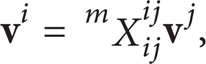
Using the recursive approach, the spatial velocity vector of a descendent body could be written using the parent spatial velocity as follows:

${\mathbf{v}}_{\mathrm{0}j,\mathrm{0}}^{\mathrm{0}}={\mathbf{v}}_{\mathrm{0}i,\mathrm{0}}^{\mathrm{0}}+{\mathbf{v}}_{ij,\mathrm{0}}^{\mathrm{0}}={\mathbf{v}}_{\mathrm{0}i,\mathrm{0}}^{\mathrm{0}}+{{}^{m}X}_{\mathrm{0}j}^{\mathrm{0}j}{\mathbf{h}}_{j,j}^j{\dot{\mathbf{q}}}_j.$

(6)

If all the bodies in the system shown in Figure 1 are considered rigid bodies, the velocity of body l could be written in a similar way as follows:

${\mathbf{v}}_{\mathrm{0}l,l}^l={{}^{m}X}_{lj}^{lj}{\mathbf{v}}_{\mathrm{0}j,j}^j+{\mathbf{h}}_{l,l}^l{\dot{\mathbf{q}}}_l.$

(7)

Rearranging the terms in the velocity equations, the system velocity could be calculated recursively as follows [12]:

$\left[\begin{array}{ccc}I& \mathrm{0}& \mathrm{0}\\ -X_{ji}^{ji}& I& \mathrm{0}\\ \mathrm{0}& -X_{lj}^{lj}& I\end{array}\right]\left[\begin{array}{c}{\mathbf{v}}_{oi,i}^i\\ {\mathbf{v}}_{oj,j}^j\\ {\mathbf{v}}_{ol,l}^l\end{array}\right]=\left[\begin{array}{ccc}{\mathbf{h}}_{i,i}^i& \mathrm{0}& \mathrm{0}\\ \mathrm{0}& {\mathbf{h}}_{j,j}^j& \mathrm{0}\\ \mathrm{0}& \mathrm{0}& {\mathbf{h}}_{l,l}^l\end{array}\right]\left[\begin{array}{c}{\dot{\mathbf{q}}}_i\\ {\dot{\mathbf{q}}}_j\\ {\dot{\mathbf{q}}}_l\end{array}\right].$

(8)

The system recursive equation for the local velocity in (8) could be written in a compact form as follows:

$T_a^{\ell \ell }{\mathbf{v}}_a^{\ell }={\mathbf{H}}_a^{\ell }{\dot{\mathbf{q}}}_a={\mathbf{v}}_r^{\ell },$

(9)

where T _a ^ℓℓ is the topological matrix and it could be easily constructed using the connectivity graph and the parent child list, the superscript ℓ refers to local matrices, the superscript a refers to the system assembly matrix, and ${\mathbf{H}}_a^{\ell }$ is the assembly influence coefficient matrices grouped in blocks corresponding to the joints’ DoF.

Similarly, the spatial acceleration vector of body j could be obtained by differentiating the velocity vector as in (9) as follows:

$\begin{array}{c}{\mathbf{a}}_{\mathrm{0}j,\mathrm{0}}^{\mathrm{0}}={\mathbf{a}}_{\mathrm{0}i,\mathrm{0}}^{\mathrm{0}}+{\mathbf{a}}_{ij,\mathrm{0}}^{\mathrm{0}},\hspace{1em}\text{where}\hspace{0.17em}\hspace{0.17em}{\mathbf{a}}_{ij,\mathrm{0}}^{\mathrm{0}}={\mathbf{h}}_{j,\mathrm{0}}^{\mathrm{0}}{\ddot{\mathbf{q}}}_j+{\tilde{\mathbf{v}}}_{\mathrm{0}j,\mathrm{0}}^{\mathrm{0}}{\mathbf{h}}_{j,\mathrm{0}}^{\mathrm{0}}{\dot{\mathbf{q}}}_j.\end{array}$

(10)

Assuming that the quadratic velocity term could be expressed as ${\mathbf{\gamma }}_{\mathrm{0}j,\mathrm{0}}^{\mathrm{0}}={\tilde{\mathbf{v}}}_{\mathrm{0}j,\mathrm{0}}^{\mathrm{0}}{\mathbf{h}}_{j,\mathrm{0}}^{\mathrm{0}}{\dot{\mathbf{q}}}_j={\tilde{\mathbf{v}}}_{\mathrm{0}j,\mathrm{0}}^{\mathrm{0}}{\mathbf{v}}_{\mathrm{0}j,\mathrm{0}}^{\mathrm{0}}$ , the global acceleration vector could written as follows:

${\mathbf{a}}_{\mathrm{0}j,\mathrm{0}}^{\mathrm{0}}={\mathbf{a}}_{\mathrm{0}i,\mathrm{0}}^{\mathrm{0}}+{\mathbf{a}}_{ij,\mathrm{0}}^{\mathrm{0}}={\mathbf{a}}_{\mathrm{0}i,\mathrm{0}}^{\mathrm{0}}+{\mathbf{h}}_{j,\mathrm{0}}^{\mathrm{0}}{\ddot{\mathbf{q}}}_j+{\mathbf{\gamma }}_{\mathrm{0}j,\mathrm{0}}^{\mathrm{0}}.$

(11)

The recursive form to calculate the system local accelerations could be written as follows:

$T_a^{\ell \ell }{\mathbf{a}}_a^{\ell }={\mathbf{H}}_a^{\ell }{\ddot{\mathbf{q}}}_a+{\dot{\mathbf{H}}}_a^{\ell }{\dot{\mathbf{q}}}_a={\mathbf{H}}_a^{\ell }{\ddot{\mathbf{q}}}_a+{\tilde{\mathbf{v}}}_r^{\ell }{\mathbf{v}}_r^{\ell }={\mathbf{H}}_a^{\ell }{\ddot{\mathbf{q}}}_a+{\mathbf{\gamma }}_a^{\ell }.$

(12)

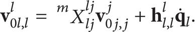
Using the kinematic equations defined earlier, the rigid body equations of motion could be derived from the momentum equations. The spatial momentum vector of the rigid body j can be written as follows:

${\mathbf{P}}_{j,G}^j=M_{j,GG}^{jj}{\mathbf{v}}_{\mathrm{0}j,G}^j,$

(13)

where ${\mathbf{P}}_{j,G}^j$ is the spatial momentum of body j, M_j,GG ^jj is the spatial mass matrix defined at the body center of mass triad G, and ${\mathbf{v}}_{\mathrm{0}j,G}^j$ is the global velocity of the triad located at the body center of mass. The centroidal spatial mass matrix is defined as follows:

$M_{j,GG}^{jj}=\left[\begin{array}{cc}{\underset{\_}{J}}_{j,GG}^{jj}& \mathrm{0}\\ \mathrm{0}& m_j\underset{\_}{I}\end{array}\right],$

(14)

where m_j is the mass body j, $\underset{\_}{I}$ is 3 × 3 identity matrix and ${\underset{\_}{J}}_{j,GG}^{jj}$ is the 3 × 3 matrix representing the body j moment of inertia defined at a triad located at the body center of mass, G. This rigid body momentum can be transformed into the global coordinate system and differentiated with respect to time to get its equation of motion as follows:

$M_{j,\mathrm{00}}^{\mathrm{00}}{\mathbf{a}}_{\mathrm{0}j,\mathrm{0}}^{\mathrm{0}}-{\tilde{\mathbf{v}}}_{\mathrm{0}j,\mathrm{0}}^{\mathrm{0}T}{M}_{j,\mathrm{00}}^{\mathrm{00}}{\mathbf{v}}_{\mathrm{0}j,\mathrm{0}}^{\mathrm{0}}={\mathbf{G}}_{j,\mathrm{0}}^{\mathrm{0}},$

(15)

where the symbol 0 refers to global coordinate system, ${\mathbf{G}}_{j,\mathrm{0}}^{\mathrm{0}}={\left[\begin{array}{cc}{\underset{\_}{\tau }}_{j,\mathrm{0}}^{\mathrm{0}}& {\underset{\_}{g}}_j^{\mathrm{0}}\end{array}\right]}^T$ is the spatial force vector including the gravitational forces, ${\underset{\_}{g}}_j^{\mathrm{0}}$ is the sum of all external forces acting of the body j, and ${\underset{\_}{\tau }}_{j,\mathrm{0}}^{\mathrm{0}}$ contains the sum of all torques and the moments of all forces about the origin of frame 0.

3. Kinematic and Dynamic Equations of Motion of Flexible Body

The dynamics of deformable body can be modeled in the multibody system as a reduced form of the full finite element model using nodal approach or modal approach. Modal formulation uses a set of kinematically admissible modes to represent the deformation of the flexible body [3–6, 22]. Component mode synthesis approach is widely used in the multibody dynamics codes to accurately simulate the flexible body dynamics in the multibody system. The main advantage of the modal formulation is that fewer elastic modes can be used to accurately capture the flexible body dynamics at reasonable computational cost. Craig-Bampton approach was introduced to account for the effect of boundary conditions and the attachment joints of the flexible body [3, 4].

The spatial gross motion of the flexible body is described by the motion of the reference frame, similar to any rigid body, using 6 coordinates. The elastic deformation of the flexible body is described by a set of constant admissible elastic modes and time-dependent modal amplitudes. This set of generalized coordinates is used to derive the modal equations of motion from the body's kinetic energy. Assuming that the flexible body reference global position is defined by ${\underset{\_}{r}}_{\mathrm{0}r}^{\mathrm{0}}$ , the orientation of flexible body is described by ${\underset{\_}{\theta }}_{\mathrm{0}r}^r$ , and the time-dependent set of elastic modal coordinates are $q_{em}^{}$ , the generalized coordinates of the flexible body can be written as

$\mathbf{q}={\left[\begin{array}{ccc}{\underset{\_}{\theta }}_{\mathrm{0}r}^r& {\underset{\_}{r}}_{\mathrm{0}r}^{\mathrm{0}}& q_{em}^{}\end{array}\right]}^T.$

(16)

Assuming that the number of modal elastic modal coordinates of body j is n _j ^m , the flexible body generalized coordinates will be 6 + n _j ^m . The velocity and acceleration vectors of the flexible body could be obtained by differentiating (16) with respect to time as follows:

$\dot{\mathbf{q}}={\left[\begin{array}{ccc}{\underset{\_}{\omega }}_{\mathrm{0}r}^r& {\dot{\underset{\_}{r}}}_{\mathrm{0}r,r}^{\mathrm{0}}& {\dot{q}}_{em}^{}\end{array}\right]}^T;\hspace{1em}\hspace{1em}\ddot{\mathbf{q}}={\left[\begin{array}{ccc}{\dot{\underset{\_}{\omega }}}_{\mathrm{0}r}^r& {\ddot{\underset{\_}{r}}}_{\mathrm{0}r,r}^{\mathrm{0}}& {\ddot{q}}_{em}^{}\end{array}\right]}^T.$

(17)

During the modal reduction of the finite element, the retained modes should be carefully selected based on the application and desired analysis [2, 4–6]. In the case of heavy structures, it may be important to retain the static interface modes and the inertia relief modes while in the case of light fabrications the natural vibration modes and the attachment modes become very important in order to achieve accurate results. The static modes could be obtained from the finite element solver by applying a unit load at the prespecified DoF and solving for the deformed shape. The normal modes are obtained by solving the eigenvalue problem for the finite element model. The attachment modes are obtained by applying a unit displacement at the prespecified attachment DoF and solving for the resulting deformed shape. The combined set of modes should be orthonormalized in order to obtain a set of kinematically independent modes in order to avoid singularities. Assuming the total mode set for body j is defined by the matrix Sj that contains number n _j ^m columns corresponding to the total number of modes and nndof rows corresponding to the number of DoF of all the nodes needed during the dynamic simulation. The matrix Sj could be regarded as blocks of rows, where each block corresponds to certain node and each row in this block is an interpolation function of the mode shape that determines the elastic deformation in certain DoF of the that node.

Assuming a triad is attached to node p. In the undeformed configuration the node is located at distance ${\underset{\_}{r}}_{rp}^r$ from the body reference and the triad is originally parallel to the body reference frame. During the dynamic simulation under the effect of dynamic loads, the flexible body deforms. The resulting elastic rotational and translational deformation at node p and first and second time derivatives are obtained using the modal transformation matrix as follows:

$\begin{array}{c}\left[\begin{array}{c}{\underset{\_}{\theta }}_p^r\\ {\underset{\_}{u}}_p^r\end{array}\right]=\left[\begin{array}{c}{S}_{jp}^r\\ S_{jp}^t\end{array}\right]q_{em}^{};\hspace{1em}\hspace{1em}\left[\begin{array}{c}{\underset{\_}{\omega }}_p^r\\ {\dot{\underset{\_}{u}}}_p^r\end{array}\right]=\left[\begin{array}{c}{S}_{jp}^r\\ S_{jp}^t\end{array}\right]{\dot{q}}_{em}^{};\\ \left[\begin{array}{c}{\dot{\underset{\_}{\omega }}}_p^r\\ {\ddot{\underset{\_}{u}}}_p^r\end{array}\right]=\left[\begin{array}{c}{S}_{jp}^r\\ S_{jp}^t\end{array}\right]{\ddot{q}}_{em}^{},\end{array}$

(18)

where quantity ${\underset{\_}{\theta }}_p^r$ represents the small elastic rotational deformation at node p relative to the body-fixed Cartesian frame r, ${\underset{\_}{u}}_p^r$ represents the elastic translational deformation at node p relative to frame r as a result of elastic deformation, and S _jp ^r and S _jp ^t represent rows of the modal transformation matrix that corresponds to the rotational and translational degrees of freedom at node p, respectively, of body j.

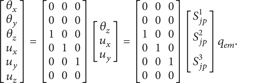
It should be noted that (18) is expressed in spatial algebra notation which implies that node p will have 3 rotational and 3 translational coordinates. In the finite element model, depending on the type of element used, the nodes may not have 6-DoF and the corresponding modal matrix block will be missing some rows. In order to be consistent in developing the equation of motion we assume that the modal block will be expanded to have 6 rows by inserting rows of zeros corresponding to the missing node DoF as follows:

$S_{jp}⟵\stackrel{-}{U}{S}_{jp},$

(19)

where $\stackrel{-}{U}$ is the unity matrix where the columns corresponding to the missing DoF are eliminated. For example, a planar node that has translation in x and y directions and rotation around z, could be written as follows:

$\left[\begin{array}{c}{\theta }_x\\ {\theta }_y\\ {\theta }_z\\ u_x\\ u_y\\ u_z\end{array}\right]=\left[\begin{array}{ccc}0& 0& 0\\ 0& 0& 0\\ 1& 0& 0\\ 0& 1& 0\\ 0& 0& 1\\ 0& 0& 0\end{array}\right]\left[\begin{array}{c}{\theta }_z\\ u_x\\ u_y\end{array}\right]=\left[\begin{array}{ccc}0& 0& 0\\ 0& 0& 0\\ 1& 0& 0\\ 0& 1& 0\\ 0& 0& 1\\ 0& 0& 0\end{array}\right]\left[\begin{array}{c}{S}_{jp}^1\\ S_{jp}^2\\ S_{jp}^3\end{array}\right]q_{em}.$

(20)

The angular and translational velocity at node p could be calculated as follows:

$\begin{array}{c}{\underset{\_}{\omega }}_{0p}^r={\underset{\_}{\omega }}_{0r}^r+S_{jp}^r{\dot{q}}_{em},\\ {\underset{\_}{\dot{r}}}_{0p,p}^r={\underset{\_}{\dot{r}}}_{0r,r}^r+{\underset{\_}{\omega }}_{0r}^r\times \left({\underset{\_}{r}}_{rp}^r+{\underset{\_}{u}}_p^r\right)+{\underset{\_}{\dot{u}}}_p^r={\left(R^{0r}\right)}^T{\underset{\_}{\dot{r}}}_{0r,r}^0+{\underset{\_}{\omega }}_{0r}^r\left({\underset{\_}{\tilde{r}}}_{rp}^r+{\underset{\_}{\tilde{u}}}_p^r\right)+S_{jt}^r{\dot{q}}_{em}.\end{array}$

(21)

The spatial velocity vector of node p could be expressed in matrix form as follows:

${\mathbf{v}}_{0p,p}^r=\left[\begin{array}{ccc}I& 0& S_{jp}^r\\ -\left({\widetilde{\underset{\_}{r}}}_{rp}^r+{\widetilde{\underset{\_}{u}}}_p^r\right)& I& S_{jp}^t\end{array}\right]\left[\begin{array}{c}{\underset{\_}{\omega }}_{0r}^r\\ {\underset{\_}{R}}^{0rT}{\dot{\underset{\_}{r}}}_{0r,r}^0\\ {\dot{q}}_{em}^{}\end{array}\right].$

(22)

Using a lumped mass approximation for the pth node, the kinetic energy can be expressed as follows:

$T_p^{}=\frac{1}{2}{\left[\begin{array}{c}{\underset{\_}{\omega }}_{0r}^r\\ {\underset{\_}{R}}^{0rT}{\underset{\_}{\dot{r}}}_{0r,r}^0\\ {\dot{q}}_{em}^{}\end{array}\right]}^T\left[\begin{array}{cc}I& \left({\widetilde{\underset{\_}{r}}}_{rp}^r+{\widetilde{\underset{\_}{u}}}_p^r\right)\\ 0& I\\ S_{jp}^{rT}& S_{jp}^{tT}\end{array}\right]\left[\begin{array}{cc}{\underset{\_}{J}}_{p,pp}^{rr}& 0\\ 0& m_{p}I\end{array}\right]\times \left[\begin{array}{ccc}I& 0& S_{jp}^r\\ -\left({\widetilde{\underset{\_}{r}}}_{rp}^r+{\widetilde{\underset{\_}{u}}}_p^r\right)& I& S_{jp}^t\end{array}\right]\left[\begin{array}{c}{\underset{\_}{\omega }}_{0r}^r\\ {\dot{\underset{\_}{r}}}_{0r,r}^0\\ {\dot{q}}_{em}^{}\end{array}\right],$

(23)

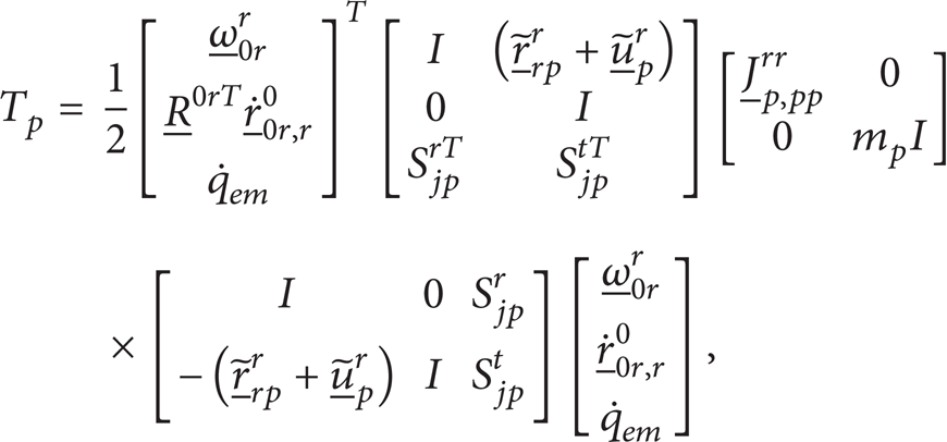
where m_p is the translational mass associated with the translational DoF at node p and ${\underset{\_}{J}}_{p,pp}^{rr}$ is the rotational inertia associated with the rotational DoF at node p, which could be simplified as follows:

$T_p^{}=\frac{1}{2}{\left[\begin{array}{c}{\underset{\_}{\omega }}_{0r}^r\\ {\underset{\_}{R}}^{0rT}{\dot{\underset{\_}{r}}}_{0r,r}^0\\ {\dot{q}}_{em}^{}\end{array}\right]}^T\left[M_{p,rr}^{rr}\right]\left[\begin{array}{c}{\underset{\_}{\omega }}_{0r}^r\\ {\underset{\_}{R}}^{0rT}{\dot{\underset{\_}{r}}}_{0r,r}^0\\ {\dot{q}}_m^{}\end{array}\right],$

(24)

where M_p,rr ^rr is the spatial inertia matrix at node p referenced to the body's reference frame r that can be identified from (24) as

$M_{p,rr}^{rr}=\left[\begin{array}{ccc}{\underset{\_}{J}}_{p,pp}^{rr}-m_p{\left({\widetilde{\underset{\_}{r}}}_{rp}^r+{\widetilde{\underset{\_}{u}}}_p^r\right)}^2& m_p\left({\widetilde{\underset{\_}{r}}}_{rp}^r+{\widetilde{\underset{\_}{u}}}_p^r\right)& {\underset{\_}{J}}_{p,pp}^{rr}{S}_{jp}^r+m_p\left({\widetilde{\underset{\_}{r}}}_{rp}^r+{\widetilde{\underset{\_}{u}}}_p^r\right)S_{jp}^t\\ -m_p\left({\widetilde{\underset{\_}{r}}}_{rp}^r+{\widetilde{\underset{\_}{u}}}_p^r\right)& m_{p}I& m_p{S}_{jp}^t\\ S_{jp}^{rT}{\underset{\_}{J}}_{p,pp}^{rr}-m_p{S}_{jp}^{tT}\left({\widetilde{\underset{\_}{r}}}_{rp}^r+{\widetilde{\underset{\_}{u}}}_p^r\right)& m_p{S}_{jp}^{tT}& S_{jp}^{rT}{\underset{\_}{J}}_{p,pp}^{rr}{S}_{jp}^r+m_p{S}_{jp}^{tT}{S}_{jp}^t\end{array}\right].$

(25)

The inertia matrix in (25) is expressed in the body's local frame r and depends on the modal coordinates $q_{em}^{}$ through ${\underset{\_}{u}}_p^r=S_{jp}^t{q}_{em}^{}$ . The kinetic energy in (24) is summed over all nodes giving the kinetic energy of the flexible body as follows:

$\begin{array}{c}T=\frac{1}{2}{\left[\begin{array}{c}{\underset{\_}{\omega }}_{0r}^r\\ {\underset{\_}{R}}^{0rT}{\dot{\underset{\_}{r}}}_{0r,r}^0\\ {\dot{q}}_{em}^{}\end{array}\right]}^T\left[\begin{array}{ccc}{M}_{\theta \theta }^{}& M_{\theta t}^{}& M_{\theta m}^{}\\ M_{\theta t}^T& M_{tt}^{}& M_{tm}^{}\\ M_{\theta m}^T& M_{tm}^T& M_{mm}^{}\end{array}\right]\left[\begin{array}{c}{\underset{\_}{\omega }}_{0r}^r\\ {\underset{\_}{R}}^{0rT}{\dot{\underset{\_}{r}}}_{0r,r}^0\\ {\dot{q}}_{em}^{}\end{array}\right]\\ =\frac{1}{2}{\dot{q}}^T\left[\begin{array}{ccc}{M}_{\theta \theta }^{}& M_{\theta t}^{}& M_{\theta m}^{}\\ M_{\theta t}^T& M_{tt}^{}& M_{tm}^{}\\ M_{\theta m}^T& M_{tm}^T& M_{mm}^{}\end{array}\right]\dot{q},\end{array}$

(26)

where

$\left[\begin{array}{ccc}{M}_{\theta \theta }^{}& M_{\theta t}^{}& M_{\theta m}^{}\\ M_{\theta t}^T& M_{tt}^{}& M_{tm}^{}\\ M_{\theta m}^T& M_{tm}^T& M_{mm}^{}\end{array}\right]=\left[\begin{array}{ccc}{\displaystyle \sum }_{p=\mathrm{1}}^n\left({\underset{\_}{J}}_{p,pp}^{rr}-m_p{\left({\widetilde{\underset{\_}{r}}}_{rp}^r+{\widetilde{\underset{\_}{u}}}_p^r\right)}^{\mathrm{2}}\right)& {\displaystyle \sum }_{p=\mathrm{1}}^n{m}_p\left({\widetilde{\underset{\_}{r}}}_{rp}^r+{\widetilde{\underset{\_}{u}}}_p^r\right)& {\displaystyle \sum }_{p=\mathrm{1}}^n\left({\underset{\_}{J}}_{p,pp}^{rr}{S}_{jp}^r+m_p\left({\widetilde{\underset{\_}{r}}}_{rp}^r+{\widetilde{\underset{\_}{u}}}_p^r\right)S_{jp}^t\right)\\ -{\displaystyle \sum }_{p=\mathrm{1}}^n{m}_p\left({\widetilde{\underset{\_}{r}}}_{rp}^r+{\widetilde{\underset{\_}{u}}}_p^r\right)& {\displaystyle \sum }_{p=\mathrm{1}}^n{m}_{p}I& {\displaystyle \sum }_{p=\mathrm{1}}^n{m}_p{S}_p^t\\ {\displaystyle \sum }_{p=\mathrm{1}}^n\left(S_{jp}^{rT}{\underset{\_}{J}}_{p,pp}^{rr}-m_p{S}_{jp}^{tT}\left({\widetilde{\underset{\_}{r}}}_{rp}^r+{\widetilde{\underset{\_}{u}}}_p^r\right)\right)& {\displaystyle \sum }_{p=\mathrm{1}}^n{m}_p{S}_{jp}^{tT}& {\displaystyle \sum }_{p=\mathrm{1}}^n\left(S_{jp}^{rT}{\underset{\_}{J}}_{p,pp}^{rr}{S}_{jp}^r+m_p{S}_{jp}^{tT}{S}_{jp}^t\right)\end{array}\right].$

(27)

It should be noted that this matrix is square symmetric with dimensions $(6+n_j^m)\times (6+n_j^m)$ . The kinetic energy expression in (26) could be used to derive the equation of motion of the modal flexible body. This mass matrix accounts for the effect of the geometric nonlinearities due to the large rotation of the components of the multibody system. Deriving the body equations of motion requires differentiating the inertia matrices in (27) with respect to time. It should be noted that the terms in mass matrix are not constant since the three matrices, $M_{\theta \theta }^{}$ , $M_{\theta t}^{}$ , and $M_{\theta m}^{}$ , depend on modal coordinates through ${\widetilde{\underset{\_}{u}}}_p^r$ and they will need to be calculated every time step using the new modal coordinates. In the meantime, the matrices $M_{tt}^{}$ , $M_{tm}^{}$ , and $M_{mm}^{}$ are constant matrices. It had been shown that a set of the inertia shape invariants could be identified and precomputed during a preprocessing stage before the dynamic simulation. During the simulation the ISI could be reused [5, 6, 22].

In order to derive the equation of motion of the flexible body, the time derivatives of the time dependent matrices, $M_{\theta \theta }^{}$ , $M_{\theta t}^{}$ , and $M_{\theta m}^{}$ , will be needed. These time derivatives could be written as follows:

$\begin{array}{c}{\dot{M}}_{\theta \theta }^{}=-{\displaystyle \sum }_{p=1}^n{m}_p\left(\left({\widetilde{\underset{\_}{r}}}_{rp}^r+{\widetilde{\underset{\_}{u}}}_p^r\right){\widetilde{\dot{\underset{\_}{u}}}}_p^r+{\widetilde{\dot{\underset{\_}{u}}}}_p^r\left({\widetilde{\underset{\_}{r}}}_{rp}^r+{\widetilde{\underset{\_}{u}}}_p^r\right)\right),\\ {\dot{M}}_{\theta t}={\displaystyle \sum }_{p=1}^n{m}_p\hspace{0.17em}{\widetilde{\dot{\underset{\_}{u}}}}_p^r,\\ {\dot{M}}_{\theta m}^{}={\displaystyle \sum }_{p=1}^n{m}_p\hspace{0.17em}{\widetilde{\dot{\underset{\_}{u}}}}_p^r{S}_p^t.\end{array}$

(28)

From the inertia submatrices in (27), the following inertia shape invariants could be identified:

$I_{}^1={\displaystyle \sum }_{p=1}^n{\underset{\_}{J}}_{p,pp}^{rr}-m_p{\left({\widetilde{\underset{\_}{r}}}_{rp}^r\right)}^2,$

(29)

where I¹ is a 3 × 3 symmetric matrix that updates the rotational inertia at flexible body reference frame due to elastic deformation through the parallel axis theorem. Consider

$I_i^2={\displaystyle \sum }_{p=1}^n{m}_p\hspace{0.17em}{\widetilde{\underset{\_}{r}}}_{rp}^r\hspace{0.17em}{\underset{\_}{\tilde{s}}}_{jp,i}^t;\hspace{1em}i=1,\dots ,n_m^j,$

(30)

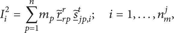
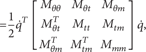
where I _i ² contains the effect of cross-coupling of elastic deformation through ${\underset{\_}{\tilde{s}}}_{jp,i}^t$ which is the skew symmetric form of the rows of the matrix S _j corresponding to the translational DoF of node p associated with mode i. This will result in n _m ^j 3 × 3 symmetric matrices:

$I_{ik}^3={\displaystyle \sum }_{p=1}^n{m}_p\hspace{0.17em}{\underset{\_}{\tilde{s}}}_{jp,i}^t\hspace{0.17em}{\underset{\_}{\tilde{s}}}_{jp,k}^t;\hspace{1em}\hspace{1em}{I}_{ki}^3=I_{ik}^{3T};\phantom{\text{hhhhh}}i=1,\dots ,n_m^j,\hspace{1em}k=i,\dots ,n_m^j,$

(31)

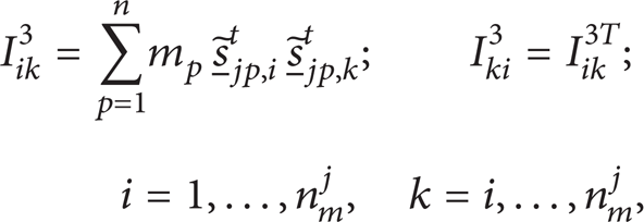
where I _ik ³ accounts for the change in the rotational inertia due to elastic deformation. This equation will result in 3 × 3 symmetric matrices when i = k:

$I_{}^4={\displaystyle \sum }_{p=1}^n{m}_{p\hspace{0.17em}}{\underset{\_}{r}}_{rp}^r\hspace{1em}\left(3\mathrm{\hspace{0.17em}\hspace{0.17em}}\text{by}\mathrm{\hspace{0.17em}\hspace{0.17em}}1\mathrm{\hspace{0.17em}\hspace{0.17em}}\text{matrix}\right),$

(32)

Equation (33) calculates I⁵ resulting in a 3 × n _m ^j matrix that could be written in the following form:

$I_i^5={\displaystyle \sum }_{p=1}^n{m}_p\hspace{0.17em}{\underset{\_}{s}}_{jp,i}^t;\hspace{1em}i=1,\dots ,n_m^j\hspace{0.17em}\hspace{0.17em}\left(\mathrm{3}\mathrm{\hspace{0.17em}\hspace{0.17em}}\text{by}\mathrm{\hspace{0.17em}\hspace{0.17em}}\mathrm{1}\mathrm{\hspace{0.17em}\hspace{0.17em}}\text{matrices}\right).$

(33)

Equation (35) calculates $I_{}^6$ resulting in 3 × n _m ^j matrix and it utilizes the inertia invariant I¹⁰:

$I_{}^5=\left[\begin{array}{cccc}{I}_1^5& I_2^5& \cdots & I_{n_m^j}^5\end{array}\right]={\displaystyle \sum }_{p=1}^n{m}_p{S}_{jp}^t,$

(34)

Equation (36) calculates I⁷ resulting in 3 × n _m ^j matrix. It should be noted that the ith column will be zero due to the cross-product:

$I_{}^6={\displaystyle \sum }_{p=1}^n\left(m_p\hspace{0.17em}{\widetilde{\underset{\_}{r}}}_{rp}^r{S}_{jp}^t+{\underset{\_}{J}}_{p,pp}^{rr}{S}_{jp}^r\right)={\displaystyle \sum }_{p=1}^n{m}_p\hspace{0.17em}{\widetilde{\underset{\_}{r}}}_{rp}^r{S}_{jp}^t+I_{}^{10}.$

(35)

Equation (38) calculates symmetric modal inertia matrix of dimensions n _m ^j × n _m ^j :

$I_i^7={\displaystyle \sum }_{p=1}^n{m}_p{\underset{\_}{\tilde{s}}}_{jp,i}^t{S}_{jp}^t;\hspace{1em}i=1,\dots ,n_m^j\begin{array}{c}\left(\mathrm{3}\mathrm{\hspace{0.17em}\hspace{0.17em}}\text{by}\mathrm{\hspace{0.17em}\hspace{0.17em}}m\mathrm{\hspace{0.17em}\hspace{0.17em}}\text{matrices};\mathrm{\hspace{0.17em}\hspace{0.17em}}i\text{th}\mathrm{\hspace{0.17em}\hspace{0.17em}}\text{column}\mathrm{\hspace{0.17em}\hspace{0.17em}}\text{is}\mathrm{\hspace{0.17em}\hspace{0.17em}}\text{zero}\right).\end{array}$

(36)

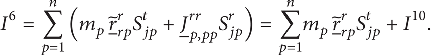
Equation (39) calculates I¹⁰ resulting in a 3 × n _m ^j matrix that could be written in the following form:

$I_{}^8={\displaystyle \sum }_{p=1}^n{m}_p\hspace{1em}\left(\text{scalar}\right),$

(37)

The inertia shape invariants I¹ to I¹⁰ in (29) to (40) are calculated and stored in the preprocessing phase. During the dynamic simulation, these inertia invariants could be used to determine the terms in the flexible body mass matrix in (27) and the derivatives in (28) as follows: starting with $M_{\theta \theta }^{}={\sum }_{p=1}^n({\underset{\_}{J}}_{p,pp}^{rr}-m_p{({\widetilde{\underset{\_}{r}}}_{rp}^r+{\widetilde{\underset{\_}{u}}}_p^r)}^2)$ as

$I_{}^9={\displaystyle \sum }_{p=1}^n\left(S_{jp}^{rT}{\underset{\_}{J}}_{p,pp}^{rr}{S}_{jp}^r+m_p{S}_{jp}^{tT}{S}_{jp}^t\right).$

(38)

where

$I_i^{10}={\displaystyle \sum }_{p=1}^n{\underset{\_}{J}}_{p,pp}^{rr}\hspace{0.17em}{\underset{\_}{s}}_{jp,i}^r;\hspace{1em}i=1,\dots ,n_m^j.$

(39)

The intermediate invariants N _j ¹ in (42) were introduced because they will be used again and should be stored to improve the computational efficiency. The next submatrix is

$I_{}^{10}=\left[\begin{array}{cccc}{I}_1^{10}& I_2^{10}& \cdots & I_{n_m^j}^{10}\end{array}\right]={\displaystyle \sum }_{p=1}^n{\underset{\_}{J}}_{p,pp}^{rr}{S}_{jp}^r.$

(40)

The remaining four inertia submatrices are evaluated as

$\begin{array}{c}{M}_{\theta \theta }^{}=I_{}^1-{\displaystyle \sum }_{j=1}^m\left(I_j^2+{\left(I_j^2\right)}^T\right)q_{mj}-\hspace{0.17em}{\displaystyle \sum }_{i,j=1}^m{I}_{ij}^3{q}_{mi}{q}_{mj}\\ \hspace{1em}=I_{}^1-{\displaystyle \sum }_{j=1}^m\left(I_j^2+{\displaystyle \sum }_{i=1}^m{I}_{ij}^3{q}_{mi}\right)q_{mj}-{\displaystyle \sum }_{j=1}^m{\left(I_j^2\right)}^T{q}_{mj}\\ \hspace{1em}=I_{}^1-{\displaystyle \sum }_{j=1}^m\left(N_j^1+{\left(I_j^2\right)}^T\right)q_{mj},\end{array}$

(41)

The time derivative of inertia matrices in (28) is expressed in terms of inertia invariants as

$N_j^1=I_j^2+{\displaystyle \sum }_{i=1}^{n_m^j}{I}_{ij}^3{q}_i;\hspace{1em}j=1,\dots ,n_m^j.$

(42)

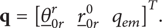
In the proposed approach, a general finite element procedure is used to determine the stiffness matrix of the flexible body. The dimension of the stiffness matrix depends on the number of finite elements and elastic coordinates. Then the modal transformation matrix is used to obtain the constant stiffness matrix that could be used during the dynamic simulation. The dimensions of the stiffness matrix depend on the number of modal coordinates used in the model reduction [23, 24]. In this section, the procedure used to formulate the flexible body stiffness matrix is briefly outlined.

The strain energy of the flexible body j could be written as the sum of the strain energies of the finite body finite elements. The strain energy of an element i of body j, U ^ij , could be written as follows:

$M_{\theta t}={\displaystyle \sum }_{p=1}^n{m}_p\left({\widetilde{\underset{\_}{r}}}_{rp}^r+{\widetilde{\underset{\_}{u}}}_p^r\right)=\widetilde{I^4}+\widetilde{I_{}^5{q}_{em}}.$

(43)

where σ ^ij and ε ^ij are the stress and strain vectors of element i of body j, respectively. In this investigation, the flexible body is assumed to undergo a small deformation, so the strain displacement relationship for small strain can be written as

$\begin{array}{c}{M}_{\theta m}^{}={\displaystyle \sum }_{p=1}^n\left({\underset{\_}{J}}_{p,pp}^{rr}{S}_{jp}^r+m_p\left({\widetilde{\underset{\_}{r}}}_{rp}^r+{\widetilde{\underset{\_}{u}}}_p^r\right)S_{jp}^t\right)=I_{}^6+{\displaystyle \sum }_{i=1}^m{I}_i^7{q}_{mi},\\ M_{tt}=I_{}^8\underset{\_}{I},\hspace{1em}\hspace{1em}{M}_{tm}^{}=I_{}^5,\hspace{1em}\hspace{1em}{M}_{mm}^{}=I_{}^9.\end{array}$

(44)

where D is a differential operator [23, 24] and ${\stackrel{-}{\mathbf{u}}}_{}^{ij}$ is the finite element nodal coordinates that include the elastic deformation which could be written as follows:

$\begin{array}{c}{\dot{M}}_{\theta t}={\displaystyle \sum }_{p=1}^n{m}_p\hspace{0.17em}{\widetilde{\dot{\underset{\_}{u}}}}_p^r=\widetilde{I^5{\dot{q}}_m}=\widetilde{M_{tm}{\dot{q}}_m},\\ {\dot{M}}_{\theta m}^{}={\displaystyle \sum }_{p=1}^n{m}_p\hspace{0.17em}{\widetilde{\dot{\underset{\_}{u}}}}_p^r\hspace{0.17em}{S}_{jp}^t={\displaystyle \sum }_{i=1}^m{I}_i^7{\dot{q}}_{mi}.\end{array}$

(45)

where ${\mathbf{r}}_{}^{ij}$ is the vector of nodal coordinates in the undeformed state and $S_{}^{ij}$ is the block of the modal transformation matrix corresponding to the element nodes. The element strain can be defined as

$U^{ij}=\frac{1}{2}{{\displaystyle \int }}_{V^{ij}}^{}{\left({\mathit{\sigma }}^{ij}\right)}^T{\mathit{\epsilon }}^{ij}d{V}^{ij},$

(46)

where q_0em ^j is the vector of initial modal coordinates that can account for initial stains in the flexible body. From the material constitutive equations, the stress-strain relationship is defined as

${\mathbf{\epsilon }}^{ij}=\mathbf{D}{\stackrel{-}{\mathbf{u}}}_{}^{ij},$

(47)

where E ^ij is the matrix of the elastic constants of the flexible body material. Using the preceding three equations, it can be shown that the strain energy of element i of the flexible body j could be written as

${\stackrel{-}{\mathbf{u}}}_{}^{ij}={\mathbf{r}}_{}^{ij}+{\mathbf{u}}_{}^{ij}={\mathbf{r}}_{}^{ij}+S_{}^{ij}{q}_{em}^j,$

(48)

where K _ff ^ij is the element stiffness matrix. The strain energy of the flexible body could be written as follows:

${\mathbf{\epsilon }}^{ij}=\mathbf{D}\left({\mathbf{r}}_{}^{ij}+S_{}^{ij}{q}_{em}^j\right)=\mathbf{D}{S}_{}^{ij}\left(q_{0em}^j+q_{em}^j\right),$

(49)

where ${\mathbf{K}}_{ff}^j$ is the flexible body stiffness matrix. Since rigid body displacements produce zero strain, the stiffness matrix of the leaf spring can be written according to the body generalized coordinate partitioning as follows:

${\mathit{\sigma }}^{ij}={\mathbf{E}}^{ij}{\mathbf{\epsilon }}^{ij},$

(50)

where the stiffness matrices associated with the reference degrees of freedom of the flexible body are equal to the null matrix. The stiffness matrix of the flexible body can be assembled and transformed using a standard finite element assembly procedure.

Similarly, the modal structural damping matrix associated with the flexible body j could be obtained and the virtual work of the flexible body damping forces could be written as follows:

$U^{ij}=\frac{1}{2}{\left(q_{em}^j\right)}^T{K}_{ff}^{ij}{q}_{em}^j,$

(51)

where Q _d is the vector of damping forces due to elastic deformation which can be written as follows:

$U^j={\displaystyle \sum }_{i=1}^{n_e^j}{U}^{ij}=\frac{1}{2}{\left({\mathbf{q}}_{em}^j\right)}^T{\mathbf{K}}_{ff}^j{\mathbf{q}}_{em}^j,$

(52)

where C _ff ^j is the modal structural damping matrix of the flexible body j.

The Lagrangian function for the flexible body could be expressed in terms of the kinetic energy T and the potential energy V as follows:

${\mathbf{K}}^j=\left[\begin{array}{ccc}\mathit{0}& \mathit{0}& \mathit{0}\\ \mathit{0}& \mathit{0}& \mathit{0}\\ \mathit{0}& \mathit{0}& {\mathbf{K}}_{ff}^j\end{array}\right],$

(53)

The equation of motion of the flexible body could be obtained by differentiating the Lagrangian operator, ℒ, using Lagrange's equation as follows [1]:

$\delta W^j={\left(Q_d\right)}^T\delta q_j^{},$

(54)

where T is the kinetic energy of the flexible body defined by (26), V is the potential energy of the flexible body (53), and $\dot{\mathbf{q}}={\left[\begin{array}{ccc}{\underset{\_}{\omega }}_{0r}^r& {\dot{\underset{\_}{r}}}_{0r}^0& {\dot{q}}_{em}^{}\end{array}\right]}^T$ . It should be noted that rigid body motion does not contribute to the potential energy function which mainly depends on the elastic deformation. In order to be able to differentiate the kinetic energy expression, the direction cosine matrix ${\underset{\_}{R}}^{0r}$ needs to be differentiated with respect to time. Also, the kinetic energy expression needs to be differentiated with respect to the orientation parameters which do not exist in the spatial algebra expression. Following the same approach by Cameron and Book [25] and Papastavridis [26], the Lagrange's equation could be expressed as follows:

$Q_d=\left[\begin{array}{ccc}0& 0& 0\\ 0& 0& 0\\ 0& 0& C_{ff}^j\end{array}\right]\left[\begin{array}{c}{\underset{\_}{\omega }}_{0r}^r\\ {\dot{\underset{\_}{r}}}_{0r}^0\\ {\dot{q}}_{em}^j\end{array}\right]=C_{}^j{\dot{q}}_{}^j,$

(55)

Performing the full differentiation and rearranging the terms in (57) we can write the equation of motion of the flexible body as follows:

$ℒ=T+V.$

(56)

where the right hand side of the equation represents the inertia forces and quadratic forces associated with the flexible body and could be written as follows:

$\frac{d}{dt}\left(\frac{\partial T}{\partial {\dot{q}}_j}\right)-\frac{\partial T}{\partial q_j}+\frac{\partial V}{\partial q_j}=Q_j,$

(57)

where K _m is the modal stiffness matrix and C _m is the modal damping matrix. The flexible body inertia and quadratic forces could be expressed in terms of the ISI as follows:

$\frac{d}{dt}\left(\frac{\partial T}{\partial {\omega }_{0r}^r}\right)+{\tilde{\omega }}_{0r}^r\left(\frac{\partial T}{\partial {\omega }_{0r}^r}\right)-\left(\frac{\partial T}{\partial {\theta }_{0r}^r}\right).$

(58)

where the new quantity N² could be expressed as follows:

$\left[\begin{array}{ccc}{M}_{\theta \theta }^{}& M_{\theta t}^{}& M_{\theta m}^{}\\ M_{\theta t}^T& M_{tt}^{}& M_{tm}^{}\\ M_{\theta m}^T& M_{tm}^T& M_{mm}^{}\end{array}\right]\left[\begin{array}{c}{\dot{\underset{\_}{\omega }}}_{0r}^r\\ {\ddot{\underset{\_}{r}}}_{0r,r}^r\\ {\ddot{q}}_{em}^{}\end{array}\right]=\left[\begin{array}{c}{Q}_{\theta }\\ Q_t\\ Q_m\end{array}\right],$

(59)

Using the inertia shape invariants in I¹ to I¹⁰, N¹, and N², the equation of motion of the flexible body is completed in (59) and ready to be integrated in the system equation of motion. In order to be consistent with the rigid body equation of motion in (15), the terms of the flexible body equation of motion could be rearranged as follows:

$\begin{array}{c}{Q}_{\theta }=-{\underset{\_}{\tilde{\omega }}}_{0r}^r{M}_{\theta \theta }^{}{\underset{\_}{\omega }}_{0r}^r-{\dot{M}}_{\theta \theta }^{}{\underset{\_}{\omega }}_{0r}^r-{\dot{M}}_{\theta t}^{}{\underset{\_}{\dot{t}}}_{0r}^r-{\underset{\_}{\tilde{\omega }}}_{0r}^r{M}_{\theta m}^{}{\dot{q}}_{em},\\ Q_t=-{\underset{\_}{\tilde{\omega }}}_{0r}^r{M}_{\theta t}^T{\underset{\_}{\omega }}_{0r}^r-2{\dot{M}}_{\theta t}^T{\underset{\_}{\omega }}_{0r}^r,\\ Q_m=-{\displaystyle \sum }_{p=1}^n{m}_p{S}_{jp}^{tT}{\left({\underset{\_}{\tilde{\omega }}}_{0r}^r\right)}^2\left({\widetilde{\underset{\_}{r}}}_{rp}^r+{\widetilde{\underset{\_}{u}}}_p^r\right)-2{\dot{M}}_{\theta m}^T\hspace{0.17em}{\underset{\_}{\omega }}_{0r}^r+K_m{q}_{em}+C_m{\dot{q}}_{em},\end{array}$

(60)

where r refers to the flexible body's local reference frame, m refers to flexible or elastic coordinates, M_j,jj ^jj represents the 6 × 6 inertia matrix associated with the reference motion of body j defined at the reference of body j (similar to the rigid body inertia matrix), $M_{}^{rm}$ , $M_{}^{mr}$ are the inertia coupling terms between the reference motion and the elastic coordinates, $M_{}^{mm}$ is the inertia matrix associated with the elastic coordinates, ${\mathbf{a}}_{0j,j}^j$ is the reference frame acceleration in the Cartesian space, and ${\ddot{q}}_{em}^{}$ represents the elastic accelerations measured relative to that frame.

4. Multibody System Equations of Motion

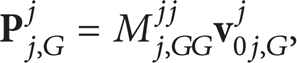
The proposed formulation utilizes the connectivity graph and parent-child list to optimize the recursive dynamics approach for solving the equations of motion. The solution is done in two steps: (1) marching forward from the root body to evaluate the velocities and accelerations of the descendent bodies through the joint variables and (2) stepping backward from each descendent body to project the Cartesian forces and the Cartesian inertia matrix into its joint subspace and into its parent body. As shown in Figure 2, the flexible body could be anywhere in the kinematic tree and could have more than one connected descendent. Descendants of the flexible body are connected through triads attached to flexible nodes. The node elastic deformation leads to extra articulation at the joint and must be accounted for during the spatial recursive calculations. The descendent bodies should be first referenced to the connecting node which is referenced to flexible body reference frame. In reference to Figure 1, the spatial transformation matrix between the flexible body j and the descendent body l could be written as follows:

$\begin{array}{c}{Q}_{\theta }=-{\underset{\_}{\tilde{\omega }}}_{0r}^r{M}_{\theta \theta }^{}{\underset{\_}{\omega }}_{0r}^r-\left({\underset{\_}{\tilde{\omega }}}_{0r}^r{I}^{10}-2N^2\right){\dot{q}}_{em},\\ Q_t=-\left(2{\dot{M}}_{\theta t}^T+{\underset{\_}{\tilde{\omega }}}_{0r}^r{M}_{\theta t}^T\right){\underset{\_}{\omega }}_{0r}^r,\\ Q_m=-\left(2{\dot{M}}_{\theta m}^T+2N^2\right){\underset{\_}{\omega }}_{0r}^r+K_m{q}_{em}+C_m{\dot{q}}_{em},\end{array}$

(61)

where X _jc ^jc is the spatial transformation matrix from the flexible body reference to the connecting node that includes the effect of the elastic translational and rotational deformations and X _cl ^cl is the spatial transformation matrix between the descendent body and the connecting node due to joint articulation. For simplicity the intermediate transformation will be omitted with the understanding that it has to be calculated. Similarly, the velocity of the descendent of the flexible body could be calculated as follows:

$N_j^2=N_j^1{\underset{\_}{\omega }}_{0r}^0,\hspace{1em}\hspace{1em}{N}^2=\left[\begin{array}{cccc}{N}_1^2& N_2^2& \cdots & N_{n_m^j}^2\end{array}\right].$

(62)

where ${\mathbf{v}}_{jc,c}^c=S_{jc}{\dot{q}}_m$ is the deformation velocity and S _jc is the expanded block of the modal transformation matrix that corresponds to the connecting node c, as shown in (19). Similarly, the acceleration of the descendent body could be obtained by differentiating (65) as follows:

$\left[\begin{array}{cc}{M}_{j,jj}^{jj}& M^{rm}\\ M^{mr}& M^{mm}\end{array}\right]\left[\begin{array}{c}{\mathbf{a}}_{0j,j}^j\\ {\ddot{q}}_{em}\end{array}\right]=\left[\begin{array}{c}{\mathbf{G}}_{j,j}^j\\ Q_m\end{array}\right],$

(63)

where ${\mathbf{\gamma }}_{l,l}^l$ is the quadratic velocity term and it accounts for the node deformation velocity as follows:

$X_{jl}^{jl}=X_{jc}^{jc}{X}_{cl}^{cl}=\left(L_{jc}^{jc}{R}^{jc}\right)X_{cl}^{cl},$

(64)

Figure 2:

Free body diagram of two connected bodies in the multibody system.

The force projected across the joint from the descendent body into the parent flexible body should be also projected into the connecting node frame first then transformed to the flexible body reference frame in order to account for the elastic deformation. These equations could be applied to a multibody system that includes a flexible body, as shown in Figure 2. The connectivity graph of the system is also shown in Figure 2. The velocity equations could be written in matrix form as follows:

$\begin{array}{c}{\mathbf{v}}_{0l,l}^l=X_{lc}^{lc}\left(X_{cj}^{cj}{\mathbf{v}}_{0j,j}^j+{\mathbf{v}}_{jc,c}^c\right)+{\mathbf{h}}_{l,l}^l{\dot{\mathbf{q}}}_l\\ \hspace{1em}=X_{lc}^{lc}\left(X_{cj}^{cj}{\mathbf{v}}_{0j,j}^j+S_{jc}{\dot{q}}_m\right)+{\mathbf{h}}_{l,l}^l{\dot{\mathbf{q}}}_l,\end{array}$

(65)

The recursive velocity equation could be written in a compact form as follows:

${\mathbf{a}}_{0l,l}^l=X_{lj}^{lj}{\mathbf{a}}_{0i,i}^i+X_{lj}^{lj}\left(S_{jc}{\ddot{q}}_m\right)+{\mathbf{h}}_{l,l}^l{\ddot{\mathbf{q}}}_l+{\mathbf{\gamma }}_{l,l}^l,$

(66)

where T _a ^ℓℓ is the topological assembly matrix and could be constructed using the system connectivity graph, the subscript a refers to the system assembly, ${\mathbf{H}}_a^{\ell }$ is the system influence coefficient matrix, Ψ ^a is modal connectivity matrix representing the contribution of the connecting nodes modal velocity to the descendent body spatial velocity, and ${\dot{\mathbf{q}}}_m^a$ is a vector of stacked modal coordinates for all flexible bodies in the system. It should be noted that T _a ^ℓℓ and ${\mathbf{H}}_a^{\ell }$ are adjusted to accommodate the flexible body nodes. Also, it should be mentioned that T _a ^ℓℓ is a lower triangular matrix and thus has simple inverse that maintains the topological structure of the original matrix and becomes an upper triangular matrix as follows [27]:

${\mathbf{\gamma }}_{l,l}^l={\tilde{\mathbf{v}}}_{jc,j}^j\left({\mathbf{h}}_{l,l}^l{\dot{\mathbf{q}}}_l\right)+X_{lc}^{lc}{\mathbf{\gamma }}_{c,c}^c,\hspace{1em}\hspace{1em}{\mathbf{\gamma }}_{c,c}^c={\tilde{\mathbf{v}}}_{oc,c}^c\left(S_{jc}{\dot{q}}_m\right).$

(67)

Similarly, the spatial accelerations in (66) and (67) could be written in a compact form as follows:

$\begin{array}{c}\left[\begin{array}{ccccc}I& 0& 0& 0& 0\\ -X_{21}^{21}& I& 0& 0& 0\\ 0& -X_{32}^{32}& I& 0& 0\\ 0& -X_{42}^{42}& 0& I& 0\\ 0& 0& 0& -X_{54}^{54}& I\end{array}\right]\left[\begin{array}{c}\begin{array}{c}{\mathbf{v}}_{\mathrm{01,1}}^1\\ {\mathbf{v}}_{\mathrm{02,2}}^2\\ {\mathbf{v}}_{\mathrm{03,3}}^3\\ {\mathbf{v}}_{\mathrm{04,4}}^4\end{array}\\ {\mathbf{v}}_{\mathrm{05,5}}^5\end{array}\right]\\ \hspace{1em}=\left[\begin{array}{ccccc}{\mathbf{h}}_{\mathrm{1,1}}^1& 0& 0& 0& 0\\ 0& {\mathbf{h}}_{\mathrm{2,2}}^2& 0& 0& 0\\ 0& 0& {\mathbf{h}}_{\mathrm{3,3}}^3& 0& 0\\ 0& 0& 0& {\mathbf{h}}_{\mathrm{4,4}}^4& 0\\ 0& 0& 0& 0& {\mathbf{h}}_{\mathrm{5,5}}^5\end{array}\right]\left[\begin{array}{c}\begin{array}{c}{\dot{q}}_1\\ {\dot{q}}_2\\ {\dot{q}}_3\\ {\dot{q}}_4\end{array}\\ {\dot{q}}_5\end{array}\right]+\left[\begin{array}{c}0\\ 0\\ X_{4c_2}^{4c_2}{S}_{\mathrm{2,2}}\\ X_{5c_3}^{5c_3}{S}_{\mathrm{2,3}}\\ 0\end{array}\right]{\dot{q}}_m.\end{array}$

(68)

Using the free body diagram for the multibody system shown in Figure 2, the equation of motion of each body could be formulated as follows: (notice that two sets of equations are needed for each flexible body as shown in (63))

$T_a^{\ell \ell }{\mathbf{v}}_a^{\ell }={\mathbf{H}}_a^{\ell }{\dot{\mathbf{q}}}_a+{\mathrm{\Psi }}^a{\dot{\mathbf{q}}}_m^a={\mathbf{v}}_r^{\ell },$

(69)

The joint influence coefficient matrices could be used to project the joint Cartesian forces into the free joint subspace as follows:

${\left(T_a^{\ell \ell }\right)}^{-1}=\left[\begin{array}{ccccc}I& -{\left(X_{21}^{21}\right)}^T& 0& 0& 0\\ 0& I& -{\left(X_{32}^{32}\right)}^T& -{\left(X_{42}^{42}\right)}^T& 0\\ 0& 0& I& 0& 0\\ 0& 0& 0& I& -{\left(X_{54}^{54}\right)}^T\\ 0& 0& 0& 0& I\end{array}\right].$

(70)

where ${\mathbf{F}}_{j,j}^j$ is a 6 × 1 force vector in the Cartesian space and Q _j is n _d × 1 force project into the free DoF joint subspace.

The system equations of motion could be derived from the kinematic relations for the Cartesian acceleration in (71), the body equations of motion in (72), and the reaction forces in (73) and arranged in matrix form as follows:

$T_a^{\ell \ell }{\mathbf{a}}_a^{\ell }={\mathbf{H}}_a^{\ell }{\ddot{\mathbf{q}}}_a+{\mathrm{\Psi }}^a{\ddot{\mathbf{q}}}_m^a+{\tilde{\mathbf{v}}}_r^{\ell }{\mathbf{v}}_r^{\ell }={\mathbf{H}}_a^{\ell }{\ddot{\mathbf{q}}}_a+{\mathrm{\Psi }}^a{\ddot{\mathbf{q}}}_m^a+{\mathbf{\gamma }}_a^{\ell }.$

(71)

A general form for the equation of motion of multibody system with flexible bodies could be written in a compact form as follows:

$\begin{array}{c}{M}_{\mathrm{5,55}}^{55}{\mathbf{a}}_{\mathrm{05,5}}^5-{\mathbf{F}}_{\mathrm{5,5}}^5={\mathbf{G}}_{\mathrm{5,5}}^5+{\left({\tilde{\mathbf{v}}}_{\mathrm{05,5}}^5\right)}^T{M}_{\mathrm{5,55}}^{55}{\mathbf{v}}_{\mathrm{05,5}}^5,\\ M_{\mathrm{4,44}}^{44}{\mathbf{a}}_{\mathrm{04,4}}^4-{\mathbf{F}}_{\mathrm{4,4}}^4-{\left(X_{54}^{54}\right)}^T{\mathbf{F}}_{\mathrm{5,5}}^5={\mathbf{G}}_{\mathrm{4,4}}^4+{\left({\tilde{\mathbf{v}}}_{\mathrm{04,4}}^4\right)}^T{M}_{\mathrm{4,44}}^{44}{\mathbf{v}}_{\mathrm{04,4}}^4,\\ M_{\mathrm{3,33}}^{33}{\mathbf{a}}_{\mathrm{03,3}}^3-{\mathbf{F}}_{\mathrm{3,3}}^3={\mathbf{G}}_{\mathrm{3,3}}^3+{\left({\tilde{\mathbf{v}}}_{\mathrm{03,3}}^3\right)}^T{M}_{\mathrm{3,33}}^{33}{\mathbf{v}}_{\mathrm{03,3}}^3,\\ M_{22}^{22}{\mathbf{a}}_{\mathrm{02,2}}^{\mathrm{2}}+M_2^{rm}{\ddot{q}}_{em}-{\mathbf{F}}_{\mathrm{2,2}}^2-{\left(X_{42}^{42}\right)}^T{\mathbf{F}}_{\mathrm{4,4}}^4-{\left(X_{32}^{32}\right)}^T{\mathbf{F}}_{\mathrm{3,3}}^3={\mathbf{G}}_{\mathrm{4,4}}^4,\\ M_2^{mr}{\mathbf{a}}_{\mathrm{02,2}}^2+M^{mm}{\ddot{q}}_{em}-{\left(S_3^c\right)}^T{\left(X_{3c}^{3c}\right)}^T{F}_{\mathrm{3,3}}^3-{\left(S_4^c\right)}^T{\left(X_{4c}^{4c}\right)}^T{F}_{\mathrm{4,4}}^4=Q_m,\\ M_{\mathrm{1,11}}^{11}{\mathbf{a}}_{\mathrm{01,1}}^1-{\mathbf{F}}_{\mathrm{1,1}}^1+{\left(X_{21}^{21}\right)}^T{\mathbf{F}}_{\mathrm{2,2}}^2={\mathbf{G}}_{\mathrm{1,1}}^1+{\left({\mathbf{v}}_{\mathrm{01,1}}^1\right)}^T{M}_{\mathrm{1,11}}^{11}{\tilde{\mathbf{v}}}_{\mathrm{01,1}}^1.\end{array}$

(72)

where the block diagonal matrix ${\mathbf{M}}_{}^{rr}$ is composed of six by six inertia matrices that represent the Cartesian inertia matrices associated with the reference frame for the rigid and flexible bodies in the system, ${\mathbf{M}}_{}^{rm}$ is the inertia coupling terms between the modal elastic coordinates and Cartesian reference accelerations, ${\mathbf{M}}_{}^{mm}$ is a block diagonal matrix containing nodal or modal flexible body inertias, T is a lower triangular topology matrix with a unity determinant, H is a block matrix of the joint influence coefficient matrices and the descendent connection nodal coefficient matrices, a is the vector of Cartesian accelerations, f is the vector of joint reaction forces, q is the vector of joint accelerations with the appended modal coordinates, G is the vector of external forces, γ is a column matrix of 6 by 1 spatial quadratic acceleration vectors, and Q is the vector of joint forces.

The system of equations given by (75) can be easily solved for the joint accelerations and the modal coordinates accelerations. Then the Cartesian accelerations and the reaction forces could be easily computed. Since the inverse of system topology matrix T is just its transpose, manipulating the terms in (75) we can get the joint and modal accelerations as follows:

$Q_j={\mathbf{h}}_{j,j}^j{\mathbf{F}}_{j,j}^j,$

(73)

The Cartesian accelerations could be calculated as follows:

$\begin{array}{c}\left[\begin{array}{cccccccccccccccc}{M}_{\mathrm{1,11}}^1& 0& 0& 0& 0& I& -{\left(X_{21}^{21}\right)}^T& 0& 0& 0& 0& 0& 0& 0& 0& 0\\ 0& M_{22}^{22}& 0& 0& 0& 0& I& -{\left(X_{32}^{32}\right)}^T& -{\left(X_{42}^{42}\right)}^T& 0& 0& 0& M^{rm}& 0& 0& 0\\ 0& 0& M_{\mathrm{3,33}}^{33}& 0& 0& 0& 0& I& 0& 0& 0& 0& 0& 0& 0& 0\\ 0& 0& 0& M_{\mathrm{4,44}}^{44}& 0& 0& 0& 0& I& -{\left(X_{54}^{54}\right)}^T& 0& 0& 0& 0& 0& 0\\ 0& 0& 0& 0& M_{\mathrm{5,55}}^{55}& 0& 0& 0& 0& I& 0& 0& 0& 0& 0& 0\\ I& 0& 0& 0& 0& 0& 0& 0& 0& 0& -{\mathbf{H}}_{\mathrm{1,1}}^1& 0& 0& 0& 0& 0\\ -X_{21}^{21}& I& 0& 0& 0& 0& 0& 0& 0& 0& 0& -{\mathbf{H}}_{\mathrm{2,2}}^2& 0& 0& 0& 0\\ 0& -X_{32}^{32}& I& 0& 0& 0& 0& 0& 0& 0& 0& 0& -{\mathbf{H}}_{\mathrm{3,3}}^3& -{\mathrm{\Psi }}_{}^{32}& 0& 0\\ 0& -X_{42}^{42}& 0& I& 0& 0& 0& 0& 0& 0& 0& 0& 0& -{\mathrm{\Psi }}_{}^{42}& -{\mathbf{H}}_{\mathrm{4,4}}^4& 0\\ 0& 0& 0& -X_{54}^{54}& I& 0& 0& 0& 0& 0& 0& 0& 0& 0& 0& -{\mathbf{H}}_{\mathrm{5,5}}^5\\ 0& 0& 0& 0& 0& -{\left({\mathbf{H}}_{\mathrm{1,1}}^1\right)}^T& 0& 0& 0& 0& 0& 0& 0& 0& 0& 0\\ 0& 0& 0& 0& 0& 0& -{\left({\mathbf{H}}_{\mathrm{2,2}}^2\right)}^T& 0& 0& 0& 0& 0& 0& 0& 0& 0\\ 0& {\left(M^{rm}\right)}^T& 0& 0& 0& 0& 0& -{\left({\mathbf{H}}_{\mathrm{3,3}}^3\right)}^T& 0& 0& 0& 0& M^{mm}& 0& 0& 0\\ 0& 0& 0& 0& 0& 0& 0& -{\left({\mathrm{\Psi }}_{}^{32}\right)}^T& -{\left({\mathrm{\Psi }}_{}^{42}\right)}^T& 0& 0& 0& 0& 0& 0& 0\\ 0& 0& 0& 0& 0& 0& 0& 0& -{\left({\mathbf{H}}_{\mathrm{4,4}}^4\right)}^T& 0& 0& 0& 0& 0& 0& 0\\ 0& 0& 0& 0& 0& 0& 0& 0& 0& -{\left({\mathbf{H}}_{\mathrm{5,5}}^5\right)}^T& 0& 0& 0& 0& 0& 0\end{array}\right]\\ \times \left[\begin{array}{c}{\mathbf{a}}_{\mathrm{01,1}}^1\\ {\mathbf{a}}_{\mathrm{02,2}}^2\\ {\mathbf{a}}_{\mathrm{03,3}}^3\\ {\mathbf{a}}_{\mathrm{04,4}}^4\\ {\mathbf{a}}_{\mathrm{05,5}}^5\\ -{\mathbf{F}}_{\mathrm{01,1}}^1\\ -{\mathbf{F}}_{\mathrm{02,2}}^2\\ -{\mathbf{F}}_{\mathrm{03,3}}^3\\ -{\mathbf{F}}_{\mathrm{04,4}}^{,}\\ -{\mathbf{F}}_{\mathrm{05,5}}^5\\ {\ddot{\mathbf{q}}}_1\\ {\ddot{\mathbf{q}}}_2\\ {\ddot{\mathbf{q}}}_m\\ {\ddot{\mathbf{q}}}_3\\ {\ddot{\mathbf{q}}}_4\\ {\ddot{\mathbf{q}}}_5\end{array}\right]=\left[\begin{array}{c}{\mathbf{G}}_{\mathrm{01,1}}^1\\ {\mathbf{G}}_{\mathrm{02,2}}^2\\ {\mathbf{G}}_{\mathrm{03,3}}^3\\ {\mathbf{G}}_{\mathrm{04,4}}^4\\ {\mathbf{G}}_{\mathrm{05,5}}^5\\ {\mathbf{\gamma }}_{\mathrm{01,1}}^1\\ {\mathbf{\gamma }}_{\mathrm{02,2}}^2\\ {\mathbf{\gamma }}_{\mathrm{03,3}}^3\\ {\mathbf{\gamma }}_{\mathrm{04,4}}^4\\ {\mathbf{\gamma }}_{\mathrm{05,5}}^5\\ {\mathbf{Q}}_1\\ {\mathbf{Q}}_2\\ {\mathbf{Q}}_m\\ {\mathbf{Q}}_3\\ {\mathbf{Q}}_4\\ {\mathbf{Q}}_5\end{array}\right].\end{array}$

(74)

And the Cartesian joint reaction forces could be obtained from

$\left[\begin{array}{ccc}{\mathbf{M}}_{}^{rr}& {\mathbf{T}}_{}^T& {\mathbf{M}}_{}^{rm}\\ {\mathbf{T}}_{}^{}& \mathrm{0}& -\mathbf{H}\\ {\left({\mathbf{M}}_{}^{rm}\right)}^T& -{\mathbf{H}}_{}^T& {\mathbf{M}}_{}^{mm}\end{array}\right]\left[\begin{array}{c}\mathbf{a}\\ -\mathbf{f}\\ \ddot{\mathbf{q}}\end{array}\right]=\left[\begin{array}{c}\mathbf{G}\\ \mathbf{\gamma }\\ \mathbf{Q}\end{array}\right],$

(75)

$\begin{array}{c}\left({\mathbf{M}}^{mm}+{\mathbf{H}}^T\left({\mathbf{T}}^T{\mathbf{M}}^{rr}\mathbf{T}\right)\mathbf{H}+{\mathbf{H}}^T{\mathbf{T}}^T{\mathbf{M}}^{rm}+{\mathbf{M}}^{mr}\mathbf{T}\mathbf{H}\right)\ddot{\mathbf{q}}\\ \hspace{1em}=\mathbf{Q}+{\mathbf{H}}^T{\mathbf{T}}^T\mathbf{G}-{\mathbf{H}}^T\left({\mathbf{T}}^T{\mathbf{M}}^{rr}\mathbf{T}\right)\mathbf{\gamma }-{\mathbf{M}}^{mr}\mathbf{T}\mathbf{\gamma }.\end{array}$

(76)

$\mathbf{a}=\mathbf{T}\mathbf{H}\ddot{\mathbf{q}}+\mathbf{T}\mathbf{\gamma }.$

(77)

$\mathbf{f}={\mathbf{T}}^T{\mathbf{M}}^{rm}+\left({\mathbf{T}}^T{\mathbf{M}}^{aa}\mathbf{T}\right)\mathbf{H}\ddot{\mathbf{q}}-{\mathbf{T}}^T\mathbf{G}+\left({\mathbf{T}}^T{\mathbf{M}}^{aa}\mathbf{T}\right)\mathbf{\gamma }.$

(78)

The sequence of evaluating the terms in (76) to (78) could be optimized in order to minimize the computational efforts and to avoid repeated calculations.

5. Outline of the Recursive Solution Algorithm

At the beginning of the dynamic simulation, the structure of the equation of motion is determined based on a preliminary analysis of the system topology. The dependent and independent variable sets are determined using the generalized coordinate portioning approach. The solver integrates both dependent and independent variable sets and the kinematic constraints are enforced. The input states to the integrator represent the first and second time derivative of the joint variables and the output states are the joint displacements and the joint velocities. The following summarizes the structure of multibody dynamic simulation recursive algorithm.

1. Using the joint variables returned from the integrator, the Cartesian displacements, velocities, and accelerations are calculated. Forward evaluation scheme is utilized (starting from the root body to the descendent/branch bodies).

2. Update spatial quantities of the flexible body nodes using the elastic nodal displacements and velocities. The input markers in the flexible bodies and the descendent bodies are then updated.

3. Calculate the internal and external forces and apply them to the different bodies (interaction forces between bodies, driver forces, soil/terrain forces, etc.).

4. Update the flexible body inertia matrices using the inertia invariants and the current modal coordinates.

5. Transform the inertia matrices into global coordinate system.

6. Calculate the inertia forces and centrifugal and Coriolis forces in Cartesian space.

7. Propagate the external and inertia forces from the descendent bodies into their parents through the connectivity nodes.

8. Project the Cartesian forces into the body joint space.

9. Calculate the second derivatives of the joint variables.

10. Send the states to the integrator.

The algorithm utilizes a predictor-corrector integrator with variable-order interpolation polynomials and variable time step [28, 29]. This explicit integrator insures the stability of the solution and the ability to capture the high-speed impacts between the different machine parts.

6. Considerations for Pre-/Postprocessing of the Flexible Body

Flexible body dynamic simulation capability is currently available in many commercial software packages. Automatic algorithms are built in these software packages to automatically extract the required information for pre-/postprocessing. This section presents the preprocessing operations required to obtain the flexible body information necessary for the dynamic simulation using the proposed formulation. Necessary considerations include the following.

1. Optimizing the system topology and the connecting nodes: as mentioned earlier, the proposed approach uses forward scheme to calculate the velocities and acceleration of the bodies in the kinematic tree and backward scheme to project the Cartesian forces and the Cartesian inertia matrix into the body-joint subspace and the parent body. In order to maximize the efficiency of the proposed approach and minimize the projection operations, the kinematic tree could be defined such that flexible body is placed close to the root of the kinematic tree. Ordering the bodies in the kinematic tree could be done in the preprocessing step.

2. The choice of the flexible body reference frame: the flexible body reference node should be selected in order to compute the modal matrix and the inertia shape invariants.

3. The selection of mode shape sets: a critical condition for successful simulation is the choice of the mode shape sets which depend on the applied nodal forces, the degrees of freedom of the joints at the attachment nodes, and the type of analysis conducted. Including the natural vibration mode shapes is a critical condition to capture the correct deformed shapes of light structures.

4. Preparing the finite element model: in order to avoid unrealistic concentrated stress or localized deformation, rigid body elements are generated at the flexible body attachment nodes. Depending on the applied forces and contact regions, it may be necessary to generate rigid body elements (RBEs) or multiple point constraints (MPC) for this region.

During the dynamic simulation, the analyst might be interested in monitoring the stresses and strains at certain elements in order to match them with the existing measurement results. In this case, the preprocessing algorithms must extract the transformation coefficients that will directly relate the flexible body modal deformation to the selected elements’ strain and hence the stresses.

After the dynamics simulation is completed the deformation at each node could be computed using the finite element package and the resulting strain could be obtained using the element shape functions. The stresses could be easily calculated from the element constitutive relations and the calculated strain. Using the time history of the flexible body deformation allows the analyst to later perform full system stresses. The user can select certain time events that can be used in life prediction and further durability assessments.

7. Flexible Body Simulation Results

In this section, simulations results of the proposed algorithms are presented and the accuracy is compared to commercially available software packages. The simulation examples include the transient response of a cantilever beam under the effect of static load, the second example represents a pendulum falling under the effect of gravity, and the third example is a double pendulum swinging under the effect of gravity.

7.1. Cantilever Beam Transient Response

The first example simulates the transient response of a cantilever beam when a sudden load is applied to the beam tip and compares the results to the results obtained from COMSOL. The beam has length of 1.5 m, width of 0.01 m, and height of 0.015 m. The beam is made of steel that has Young's modulus of 2.06 E + 09 Pa, Poisson's ration of 0.29, and mass density of 7820 kg/m³. The beam is fixed from one end to the wall while the other end is subjected to a step load of 12 N. For the multibody dynamic simulation, the beam will be modeled as flexible body with fixed joint at the beam end. As a consequence, the body reference is selected at the node attaching the cantilever to the ground. For the preprocessing, NASTRAN is used to perform the necessary transformations and extract the mode shapes for the flexible body. The first 12 natural modes of the cantilever are selected to represent the elastic deformation of the beam and the inertia invariants are calculated based on those modes. Figure 3 shows the first 12 modes of the cantilever beam and the corresponding natural frequencies that will be used in the multibody dynamic simulation.

Figure 3:

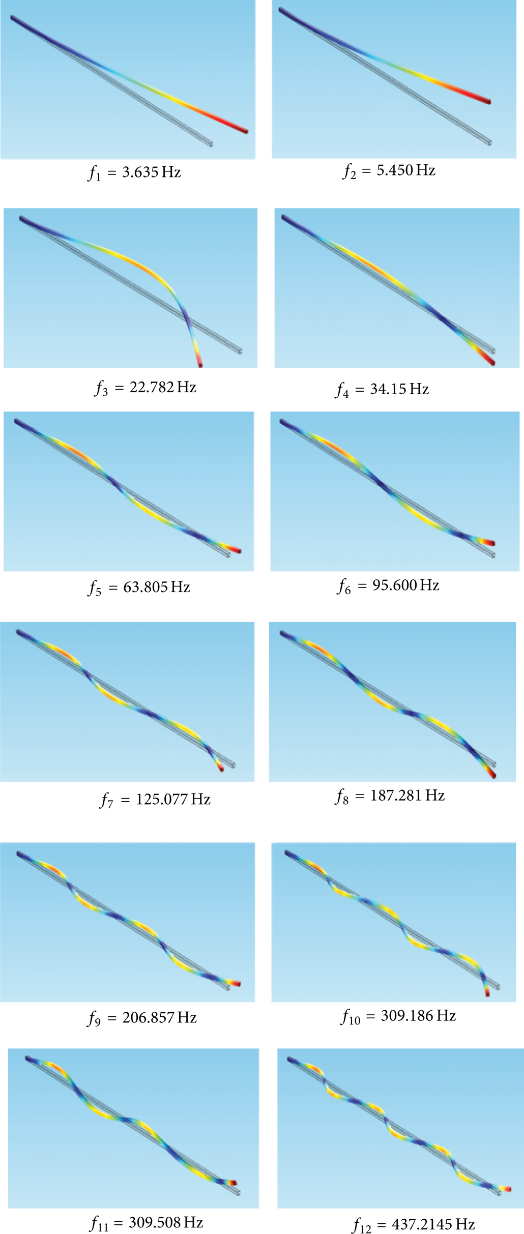
Mode shapes of the cantilever beam and the corresponding natural frequencies.

The MDB simulation utilized 12 modes to represent the flexible body while the full finite element model was used in COMSOL. Figure 4 shows the results of the dynamic tip deflection of the beam under the applied load. It could be noticed that there is very good agreement between the two sets of the results. Although 12 modes were included in the simulation, it is expected that only those modes contributing to the vertical tip deflection will be excited. Figure 5 shows an FFT of the tip deflection response, where only the first six bending modes were excited.

Figure 4:

Comparing the beam tip deflection using proposed formulation and COMSOL.

Figure 5:

Comparing FFT of the beam tip deflection using proposed formulation and COMSOL.

The stress state is another representative that captures all the information of the deformed shape. Figure 6 compares Von-Mises stresses obtained using modal approach to the stresses obtained from COMSOL. In order to eliminate the attachment effect that may give incorrect results, the stress is measured at an element that is located at distance 2h (0.03 m) from the connection node. It should be noticed that very good agreement could be achieved using the proposed algorithm.

Figure 6:

Comparing the calculated stress using proposed formulation and COMSOL.

7.2. Simple Pendulum Transient Response

The same beam in the first example was used as a pendulum to check the algorithm performance under large rotation using a pendulum model. The proposed modal formulation results were compared to the full finite element model using LS-Dyna. The pendulum is connected to the ground with a revolute joint and swinging freely under the effect of gravity. Figure 7 shows the tip deflection as the beam swings under the effect of gravity. Figure 8 shows a comparison the resulting of Von-Mises stresses measured at the same element as before. It is clear from the figure that both results are in a very good agreement.

Figure 7:

Tip deflection of the swinging pendulum at the beam tip.

Figure 8:

Von-Mises stress of swinging pendulum.

7.3. Double Pendulum Transient Response

To complete the verification of the proposed formulation and equations of motion, the projection operations of the descendent bodies into parent bodies need to be checked. This could be achieved using an articulated multibody system. The same beam in the first example was used as a double pendulum to check the projections algorithms. In the case of double pendulum, the first pendulum has two attachment points (at the two revolute joints) while the second pendulum has only one attachment point. For this reason, the boundary conditions for both modal flexible bodies will be different and this requires a different set of mode shapes for each body [30]. In the current simulation, hinged-hinged boundary conditions were used to extract the flexible body mode shapes for the first pendulum while the same mode shapes in example 1 are used for the second pendulum. The first 12 mode shapes of the first pendulum are shown in Figure 9.

Figure 9:

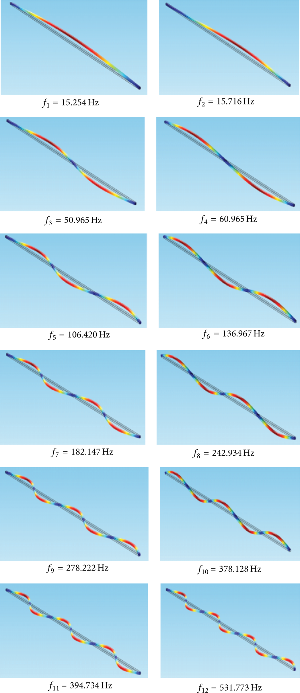
Mode shapes of the beam with hinged-hinged boundary conditions.

The pendulum is connected to the ground with a revolute joint and swinging freely under the effect of gravity. Figure 10 shows the tip deflection of the first pendulum as the beam swings under the effect of gravity while Figure 11 shows the tip deflection of the second pendulum.

Figure 10:

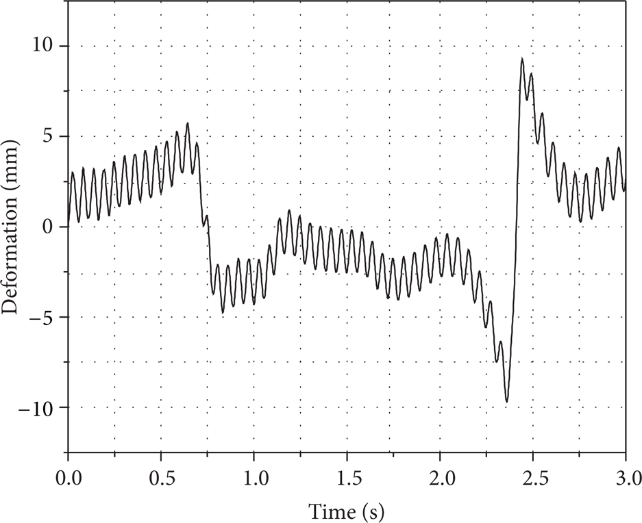
Tip deflection of the first pendulum at the beam tip.

Figure 11:

Tip deflection of the second pendulum at the beam tip.

8. Conclusions

This paper presented an approach for modeling flexible body in joint based multibody dynamics formulation. The spatial algebra was used to derive the equation of motion. Component mode synthesis approach was employed to reduce the finite element model into a set of modal coordinates. The resulting flexible body mass matrix is dependent on the generalized modal elastic coordinates. A set of inertia shape invariants were developed to efficiently update the mass matrix with minimum computational cost. The flexible body equations of motion were formulated using Cartesian coordinate system, joint variables, and the flexible body modal coordinates. The system connectivity information was to define the system topological connectivity matrix. The joint influence coefficient matrices and their dual matrices were used to project the Cartesian quantities into the joint subspace leading to the minimum set of differential equations. The structure of the equation of motion and the recursive solution algorithm were presented. The pre- and postprocessing operations required to model the flexible body were presented in this paper. The presented approach can be used to model large structures as well as light fabrications if the right set of modes were selected to represent the reduced flexible body.

Conflict of Interests

The author declares that there is no conflict of interests regarding the publication of this paper.