Sage Journals: Discover world-class research

Abstract

This paper presents a novel piezoactuator-based valve for vehicle ABS. The piezoactuator located in one side of a rigid beam makes a displacement required to control the pressure at a flapper-nozzle of the pneumatic valve. In order to obtain the wide control range of the pressure, a pressure modulator comprised of dual-type cylinder and piston is proposed. The governing equation of the piezovalve system which consists of the proposed piezoactuator-based valve and the pressure modulator is obtained. The longitudinal vehicle dynamics and the wheel slip condition are then formulated. In order to evaluate the performance of the proposed piezovalve system from the viewpoint of the vehicle ABS, a sliding mode controller is designed for wheel slip control. The tracking control performances for the desired wheel slip rate are evaluated and the braking performances in terms of braking distance are then presented on different road conditions (dry asphalt, wet asphalt, and wet jennite). It is clearly shown that the desired wheel slip rate is well achieved and the braking distance and braking time can be significantly reduced by using the proposed piezovalve system associated with the slip rate controller.

1. Introduction

Because vehicle safety is becoming increasingly important in recent years, several electronic control systems have been actively developed to enhance the vehicle safety. Especially, the antilock brake system (ABS) plays an important role in the safety and stability of the vehicle. The ABS prevents the wheel locking during the braking by controlling the braking pressure supplied to the braking pad. In general, a commercial ABS consists of the solenoid valve, check valves, accumulator, and damper chamber. However, the solenoid valve has some problems such as complex operating mechanism and high price [1]. Moreover, the ABS controlled by the solenoid valve has pulsatory motion, because the solenoid can be operated in only on/off states. Consequently, it is desirable to introduce alternative means-of-actuation mechanisms to resolve these drawbacks. One of the new approaches to achieve the required characteristics for a valve system is to use smart materials such as electrorheological (ER) fluid, magnetorheological (MR) fluid, and piezoactuator.

When the ER and MR valves are used in the servo valve system, the output pressure can be continuously controlled by controlling the intensity of the electric field or magnetic field. Because the ER and MR valves have no moving parts, the valves can be designed in a simple way. This feature of the ER and MR fluid based valve has triggered considerable research activity in the development of various valve devices [2 –10]. Simmons proposed a plate-type ER valve and the pressure drop response of the ER valve with respect to the electric field is evaluated [5]. In order to analyze the pressure drop of an ER valve, Whittle et al. formulated a second order dynamic model and experimentally evaluated the validity of the model [6]. Recently, Choi and Sung also studied the control performance of the ER valve based ABS by considering the braking force distribution [7]. They researched the slip rate control performance of a quarter-car model via both computer simulations and a hardware-in-the-loop simulation (HILS). Yoo and Wereley researched on miniaturization of the MR valve while maintaining the maximum performance of the MR effect [8]. Li et al. and Nguyen et al. investigated an optimized design of a high-efficiency MR valve using finite element analysis [9, 10].

On the other hand, there are several works on the development of new types of valve mechanisms actuated by the piezoactuator [11 –14]. Using many advantages of the piezoactuator like a fast response characteristic and large generating force, Hirata and Esashi designed the anticorrosive mass-flow valve device actuated by piezostack actuator [12]. The designed piezovalve was evaluated by doing experiment from the viewpoint of the response time and flow-rate of the valve. Tan et al. evaluated the performance of the proposed piezohydraulic actuation system with active valves [13]. Recently, Jeon et al. also investigated the pressure control performance of the piezovalve modulator [14]. They presented the pressure control performance of a proposed piezovalve model via computer simulations. However, a research work on the piezovalve system which can be applicable to vehicle ABS is considerably rare.

Consequently, the main contribution of this work is to propose a new valve system for vehicle ABS using the piezoactuator. In order to achieve this goal, the piezovalve system that consists of the piezostack actuator, the flapper-nozzle mechanism, and the pressure modulator is devised. The governing equations of a longitudinal vehicle model and wheel slip model are derived and integrated with the dynamic model of the proposed piezovalve system. Subsequently, a sliding mode controller for the slip rate tracking control is designed and implemented through a computer simulation. The braking performances of the vehicle ABS associated with the proposed piezovalve system are evaluated in terms of braking distance and wheel slip tracking results with three different kinds of road conditions.

2. Piezovalve System

The geometry of the proposed piezovalve system for controlling the braking pressure of a passenger vehicle is shown in Figure 1. The system consists of a piezostack actuator, hinge, flapper, nozzles, and pressure modulator for the amplification of the controllable pressure range. When the braking pressure needs to be increased, the flapper is pushed to the right side of the nozzle by the piezoactuator. Then, the piston will move to the left side and the output pressure P_B will be increased. On the contrary, if the flapper is pulled to the left side of the nozzle, the braking pressure will be decreased. This mechanism can control the braking pressure for vehicle ABS by controlling the applied voltage to the piezoactuator.

Figure 1:

Schematic configuration of the proposed piezovalve system.

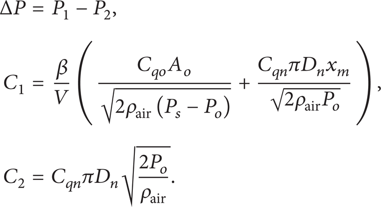
The mechanical configuration of the piezovalve is shown in Figure 2. At each nozzle, the pressure due to the supplying pressure P_s can be obtained as follows [15]:

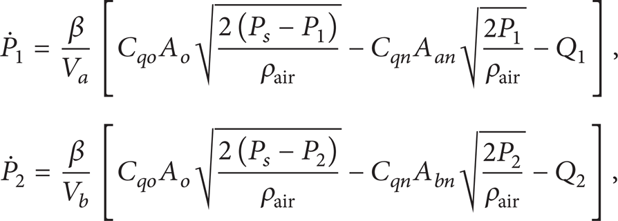
\begin{matrix} {\dot{P}}_{1} = \frac{β}{V_{a}} [C_{q o} A_{o} \sqrt{\frac{2 (P_{s} - P_{1})}{ρ_{air}}} - C_{q n} A_{a n} \sqrt{\frac{2 P_{1}}{ρ_{air}}} - Q_{1}], \\ {\dot{P}}_{2} = \frac{β}{V_{b}} [C_{q o} A_{o} \sqrt{\frac{2 (P_{s} - P_{2})}{ρ_{air}}} - C_{q n} A_{b n} \sqrt{\frac{2 P_{2}}{ρ_{air}}} - Q_{2}], \end{matrix}

(1)

where β is the bulk modulus of air and V_a and V_b are control volumes at a and b. In this work, the load flow-rates Q1 and Q2 are neglected, because they are much smaller than Q_an, Q_bn. C_qn and C_qo which are the flow coefficients at the nozzle and orifice, respectively. ρ_air is the density of air and A_o is the area of the orifice. A_an and A_bn are curtain areas at the nozzles according to the location of the flapper and are determined as follows:

A_{a n} = (x_{m} - x) π D_{n}, A_{b n} = (x_{m} + x) π D_{n},

(2)

D_n is the diameter of the nozzle and x_m is the maximum displacement of the flapper. The nonlinear equations (1) and (2) can be linearized about the equilibrium point, x = 0, as follows [1]:

Δ \dot{P} + C_{1} Δ P = 2 C_{2} x,

(3)

where

\begin{matrix} Δ P = P_{1} - P_{2}, \\ C_{1} = \frac{β}{V} (\frac{C_{q o} A_{o}}{\sqrt{2 ρ_{air} (P_{s} - P_{o})}} + \frac{C_{q n} π D_{n} x_{m}}{\sqrt{2 ρ_{air} P_{o}}}), \\ C_{2} = C_{q n} π D_{n} \sqrt{\frac{2 P_{o}}{ρ_{air}}} . \end{matrix}

(4)

Figure 2:

Mathematical model of the proposed piezovalve.

In order to amplify the displacement of the piezostack actuator, the hinge-lever mechanism is proposed. At the neighborhood of the nozzle, the displacement of the flapper can be obtained as follows:

x = - \frac{l_{2}}{l_{1}} z_{P},

(5)

l₁ is the length between the hinge and piezoactuator and l₂ is the length between the hinge and nozzle. z_p is the generated displacement by the piezoactuator. The original displacement of the piezoactuator can be calculated by [16]

z_{P} = a + b V_{p} (t),

(6)

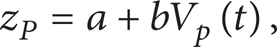
a and b are the coefficients of the piezoactuator. However, in practice, the relationship between displacement of the piezostack actuator and input voltage is not linear due to the inherent hysteresis and blocking force. In other words, a and b are treated as the uncertainties as follows:

\begin{matrix} a = a_{n} + Δ a = a_{n} (1 + γ_{1}), | γ_{1} | < ϕ_{1} < 1, \\ b = b_{n} + Δ b = b_{n} (1 + γ_{2}), | γ_{2} | < ϕ_{2} < 1, \end{matrix}

(7)

where γ₁ and γ₂ are the uncertainty ratio and ϕ₁ and ϕ₂ are the maximum range of the uncertainty of the piezostack actuator.

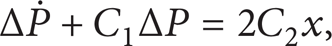
By substituting (6) into (5), the equation of the flapper can be rewritten as follows:

x = - \frac{l_{2}}{l_{1}} (a + b V_{p} (t)) .

(8)

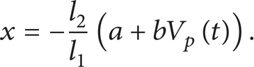
The governing equation of the piezovalve is then obtained by adding (3) and (8) as follows:

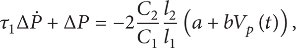
τ_{1} Δ \dot{P} + Δ P = - 2 \frac{C_{2}}{C_{1}} \frac{l_{2}}{l_{1}} (a + b V_{p} (t)),

(9)

where τ₁(= 1/C₁) is the time constant of the pneumatic valve operated by the piezoactuator.

The passenger vehicle ABS requires controllable pressure level from 100 bar to 180 bar (for dry asphalt) [17]. However, by using the proposed piezovalve with the parameters listed in Table 1, generated pressure is not enough to control the ABS. Therefore, a pressure modulator integrated with the piezovalve is proposed to obtain the suitable pressure level for vehicle ABS. The pressure modulator increases the mean value of pressure level by supplying the initial braking pressure generated by master cylinder and amplifies the controllable pressure range. As shown in Figure 3, the right cylinder is filled with air, while the left cylinder is filled with brake oil. Then, the dynamic equation of the brake line model from the modulator to the brake pad is then given by

τ_{2} {\dot{P}}_{B r} + P_{B r} = - η_{B} \frac{A_{1}}{A_{2}} Δ P + P_{B r}^{*}, τ_{2} = R_{B r} C_{B r},

(10)

where P_Br and P_Br^* present the amplified output pressure and the pressure supplied by the master cylinder, respectively. A₁ and A₂ are the area of the large piston and the small piston, respectively. R_Br is the fluid resistance of the brake line, C_Br is the fluid capacitance of the brake oil, and τ₂ is the time constant of the brake line. η_B is the influence factor on the output pressure and is chosen to be 0.5 during braking.

Table 1:

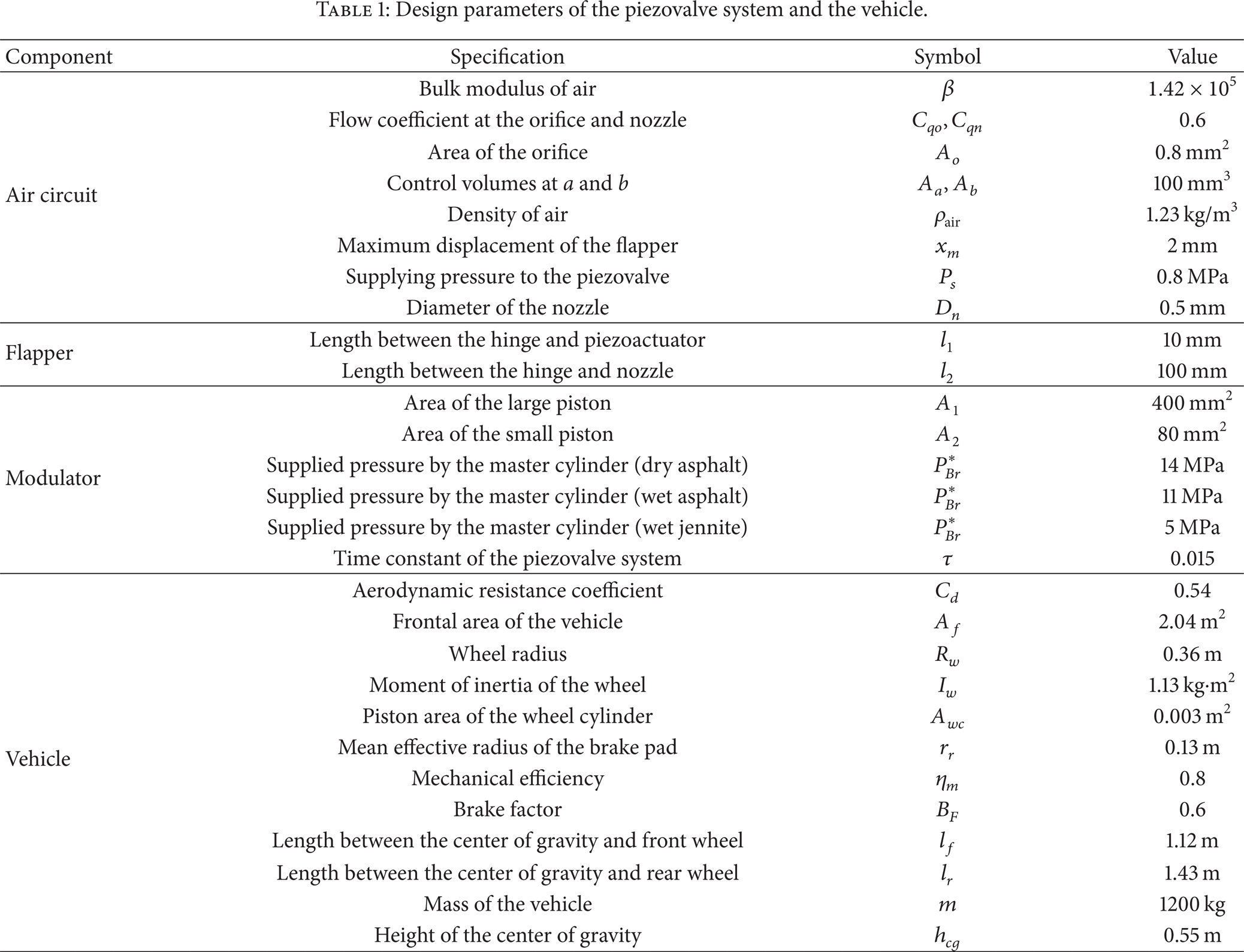
Design parameters of the piezovalve system and the vehicle.

Component	Specification	Symbol	Value

Air circuit	Bulk modulus of air	β	1.42 × 10⁵
	Flow coefficient at the orifice and nozzle	C_qo,C_qn	0.6
	Area of the orifice	A _o	0.8 mm²
	Control volumes at a and b	A_a,A_b	100 mm³
	Density of air	ρ_air	1.23 kg/m³
	Maximum displacement of the flapper	x_m	2 mm
	Supplying pressure to the piezovalve	P _s	0.8 MPa
	Diameter of the nozzle	D _n	0.5 mm

Flapper	Length between the hinge and piezoactuator	l1	10 mm
Flapper	Length between the hinge and nozzle	l2	100 mm

Modulator	Area of the large piston	A1	400 mm²
	Area of the small piston	A2	80 mm²
	Supplied pressure by the master cylinder (dry asphalt)	$P_{B r}^{*}$	14 MPa
	Supplied pressure by the master cylinder (wet asphalt)	$P_{B r}^{*}$	11 MPa
	Supplied pressure by the master cylinder (wet jennite)	$P_{B r}^{*}$	5 MPa
	Time constant of the piezovalve system	τ	0.015

Vehicle	Aerodynamic resistance coefficient	C _d	0.54
	Frontal area of the vehicle	A _f	2.04 m²
	Wheel radius	R _w	0.36 m
	Moment of inertia of the wheel	I _w	1.13 kg·m²
	Piston area of the wheel cylinder	A _wc	0.003 m²
	Mean effective radius of the brake pad	r_r	0.13 m
	Mechanical efficiency	η_m	0.8
	Brake factor	B _F	0.6
	Length between the center of gravity and front wheel	l_f	1.12 m
	Length between the center of gravity and rear wheel	l_r	1.43 m
	Mass of the vehicle	m	1200 kg
	Height of the center of gravity	h _cg	0.55 m

Figure 3:

Configuration of the pressure modulator.

By combining (9) and (10), a second order dynamic model for the piezovalve system can be obtained as follows:

τ_{1} τ_{2} {\ddot{P}}_{B r} + (τ_{1} + τ_{2}) {\dot{P}}_{B r} + P_{B r} = \frac{A_{1}}{A_{2}} \frac{C_{2}}{C_{1}} \frac{l_{2}}{l_{1}} (a + b V_{p} (t)) + P_{B r}^{*} .

(11)

However, since the time constant of the brake line τ₂ is much smaller than the time constant of piezovalve τ₁, the second order dynamic model can be reduced to the following first order dynamic model:

τ {\dot{P}}_{B r} + P_{B r} = \frac{A_{1}}{A_{2}} \frac{C_{2}}{C_{1}} \frac{l_{2}}{l_{1}} (a + b V_{p} (t)) + P_{B r}^{*}, τ = τ_{1} + τ_{2},

(12)

where τ is the time constant of the piezovalve system.

3. Wheel Slip Control Model

In this work, the precise and appropriate braking force should be achieved by turning the brake pressure through wheel slip control using the piezovalve system. When the brake pedal is pressed, the master cylinder generates the initial braking pressure. In order to satisfy the antilock condition of the vehicle, the piezovalve system generates the additive/subtractive braking pressure. The suitable additive/subtractive pressure can be calculated by using vehicle dynamics model. Figure 4 presents the longitudinal full-car dynamic model. The equation of the simplified longitudinal vehicle dynamics can be expressed by using Newton's second law:

m {\dot{V}}_{x} = - \sum_{i = 1}^{4} F_{t, i} - F_{a},

(13)

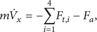
where m and V_x are the mass and longitudinal velocity of the vehicle, respectively. F_t,i is the road frictional force between each wheel and road surface. As shown in Figure 4, i means wheel numbers from front-left to rear-right for more simple denotation. F_a is the aerodynamic force affected by the shape, size, and linear velocity of the vehicle. F_a can be expressed as follows [18]:

F_{a} = \frac{ρ_{air}}{2} C_{d} A_{f} V_{x}^{2} .

(14)

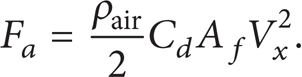
In the above, ρ_air is the density of the air, C_d is the aerodynamic resistance coefficient, and A_f is the frontal area of the vehicle. The road frictional force F_t,i can be obtained by the Coulomb law as follows:

F_{t, i} = μ (λ_{i}) F_{N, i}, i = 1,2, 3,4,

(15)

where F_N,i is the normal load at each wheel. In case of reality, the load is subject to change depending on the pitching motion of the vehicle. Assuming that there is no drastic change of the height of road surface and steering during braking operation, the approximated static model for the load on each wheel can be calculated as follows:

\begin{matrix} F_{N, 1} = F_{N, 3} = c_{11} m - c_{2} a_{x} (Front Wheel), \\ F_{N, 2} = F_{N, 4} = c_{12} m + c_{2} a_{x} (Rear Wheel), \end{matrix}

(16)

where

\begin{matrix} c_{11} = \frac{g}{2} (1 - \frac{l_{f}}{l_{f} + l_{r}}), c_{12} = \frac{g}{2} (\frac{l_{f}}{l_{f} + l_{r}}), \\ c_{2} = \frac{m \cdot h_{c g}}{2 (l_{f} + l_{r})}, \end{matrix}

(17)

where a_x is the longitudinal acceleration of the vehicle. l_f is the distance between the center of gravity and front wheel and l_r is the distance between the center of gravity and rear wheel. h_cg is the height of the center of the gravity and g is the gravitational acceleration. In (15), the longitudinal coefficient of friction μ(λ_i,V) is a nonlinear function of wheel slip rate and changes with different road conditions. Figure 5 shows this relationship between the friction coefficient and wheel slip at various road conditions which are the dry asphalt, wet asphalt, and wet jennite [19]. The peak values of the friction coefficient at every road condition are used as the reference wheel slip values in the proposed control system.

Figure 4:

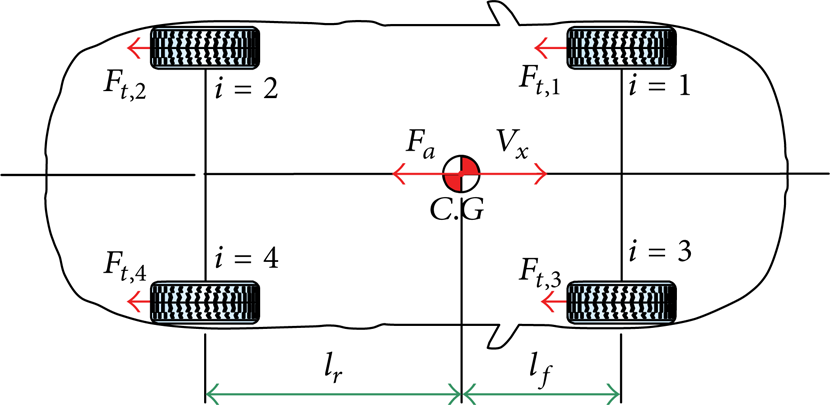
Longitudinal vehicle model.

Figure 5:

μ–λ relations for various road conditions.

During the braking, the wheel slip λ_i and the differential value of the wheel slip ${\dot{λ}}_{i}$ are established by

\begin{matrix} λ_{i} = \frac{V_{x} - {V_{w}}_{, i}}{V_{x}} = \frac{V_{x} - R_{w} ω_{i}}{V_{x}} \\ {\dot{λ}}_{i} = \frac{(a_{x} - R_{w} {\dot{ω}}_{i}) V_{x} - (V_{x} - R_{w} ω_{i}) a_{x}}{{(V_{x})}^{2}} = \frac{1}{V_{x}} ((1 - λ_{i}) a_{x} - {\dot{ω}}_{i} R_{w}), \end{matrix}

(18)

where V_w,i is the wheel speed, R_w is the wheel radius, and ω_i is the angular wheel velocity of each wheel. When the wheel slip condition is zero, the wheel and vehicle have the same velocity. On the contrary, when the wheel slip condition is one, the wheel is locked. When the wheel is locked, the vehicle is no longer steerable and has smaller frictional force than the vehicle which has appropriate wheel slip condition as shown in Figure 5. It means that the velocity of the wheel slip controlled system is more quickly decreased than the uncontrolled system.

During deceleration, because the braking torque is applied to the wheels, the speed of the wheel and the vehicle is decreased. From the wheel model shown in Figure 6, the following equation can be obtained:

I_{w} {\dot{ω}}_{i} = F_{t, i} R_{w} + T_{D, i} - T_{B, i},

(19)

where the variables of T_D,i, T_B,i, and F_t,i are the driving torque, the braking torque, and the frictional force of each wheel, respectively. The T_B,i can be calculated by

T_{B, i} = A_{w c} η_{m} B_{F} r_{r} P_{B, i} .

(20)

Figure 6:

Wheel dynamic model.

I_w is the moment of inertia of the wheel, r_r is the mean effective radius of the brake pad, A_wc is the piston area of the wheel cylinder, η_m is the mechanical efficiency, and B_F is the brake factor. During the braking operation, the driving torque T_D,i can be neglected. Then, the following dynamic models for each wheel featuring the piezovalve system are obtained by substituting (12), (19), and (20) into (18):

\begin{array}{l} {\dot{λ}}_{i} = a_{11} λ_{i} + a_{12} P_{B, i} + f_{1, i}, \\ {\dot{P}}_{B, i} = a_{22} P_{B, i} + b_{2} V_{p, i} (t) + f_{2} + \frac{1}{τ} {P_{B}}^{*}, \end{array}

(21)

where

\begin{matrix} a_{11} = - \frac{a_{x}}{V_{x}}, a_{12} = \frac{R_{ω} A_{w c} η_{m} B_{F} r_{r}}{V_{x} I_{w}}, \\ f_{1, i} = \frac{a_{x}}{V_{x}} + \frac{R_{w}^{2} F_{t, i}}{V_{x} I_{w}}, a_{22} = - \frac{1}{τ}, \\ b_{2} = \frac{b}{τ} \frac{C_{2}}{C_{1}} \frac{A_{1}}{A_{2}} \frac{l_{2}}{l_{1}}, f_{2} = \frac{a}{τ} \frac{C_{2}}{C_{1}} \frac{A_{1}}{A_{2}} \frac{l_{2}}{l_{1}} . \end{matrix}

(22)

4. Controller Design and Results

Among many control strategies, in this work, a sliding mode controller (SMC) which is very robust against parameter uncertainties is adopted, because the system has some uncertainties such as parameters of the piezostack actuator (see (7)). Because the control target is to obtain a desired wheel slip by using the proposed piezovalve system, the tracking errors are defined as follows:

e_{λ 1, i} = λ_{i} - λ_{d}, e_{λ 2, i} = {\dot{λ}}_{i} - {\dot{λ}}_{d},

(23)

where λ_d is the desired wheel slip which has generally a maximum frictional coefficient. Assuming that the acceleration of the vehicle a_x is constant during the wheel slip control, ${\dot{a}}_{11}$ and ${\dot{a}}_{12}$ can be calculated by

{\dot{a}}_{11} = a_{11}^{2}, {\dot{a}}_{12} = a_{12} a_{11} .

(24)

From (21), (23), and (24), the difference between wheel slip rate and desired wheel slip rate can be rewritten as follows:

\begin{matrix} {\dot{e}}_{λ 1, i} = e_{λ 2, i}, \\ {\dot{e}}_{λ 2, i} = - a_{11} a_{22} λ_{i} + (2 a_{11} + a_{22}) {\dot{λ}}_{i} + a_{12} b_{2} V_{p, i} (t) - (a_{11} + a_{22}) f_{1, i} + a_{12} f_{2} + \frac{a_{12}}{τ} P_{B} + {\dot{f}}_{1, i} - {\ddot{λ}}_{d} . \end{matrix}

(25)

As a first step to formulate the sliding mode controller, a sliding surface which guarantees stable sliding mode motion is chosen as follows:

S_{a, i} = C_{λ} e_{λ 1, i} + e_{λ 2, i},

(26)

where C_λ is the gradient of the sliding surface. In order to guarantee that the tracking errors e_λ1,i and e_λ2,i of the system are constrained to the sliding surface during the sliding motion, the following sliding mode condition should be satisfied:

S_{a, i} \cdot {\dot{S}}_{a, i} < 0 .

(27)

From (25), (26), and (27), the SMC is designed as follows:

V_{p, i} (t) = - \frac{1}{a_{12} b_{2}} [(2 a_{11} + a_{22} + C_{λ}) e_{λ 2, i} - a_{11} a_{22} e_{λ 1, i} + f_{i}^{'} + K_{λ} sgn (S_{i})],

(28)

where sgn⁡(·) is the signum function, K_λ is a sliding mode control gain, and f_i′ is obtained as follows:

f_{i}^{'} = - {\ddot{λ}}_{d} + (2 a_{11} + a_{22}) {\dot{λ}}_{d} - a_{22} a_{11} λ_{d} - (a_{11} + a_{22}) f_{1, i} + a_{12} f_{2} + \frac{a_{12}}{τ} P_{B} + {\dot{f}}_{1} .

(29)

The above controller has been designed by assuming that the uncertainties do not exist in the control model (21). However, as mentioned earlier, the uncertainties originated from the supplying pressure and hysteresis of the piezoactuator should be considered. Now, substituting (7) into (21) yields the following control model which contains the imposed uncertainties:

\begin{matrix} {\dot{λ}}_{i} = a_{11} λ_{i} + a_{12} P_{B, i} + f_{1, i}, \\ {\dot{P}}_{B, i} = a_{22} P_{B, i} + b_{2, n} (1 + γ_{2}) V_{p, i} (t) + f_{2, n} (1 + γ_{1}) + \frac{1}{τ} P_{B}^{*}, \end{matrix}

(30)

where

b_{2, n} = \frac{b_{n}}{τ} \frac{C_{2}}{C_{1}} \frac{A_{1}}{A_{2}} \frac{l_{2}}{l_{1}}, f_{2, n} = \frac{a_{n}}{τ} \frac{C_{2}}{C_{1}} \frac{A_{1}}{A_{2}} \frac{l_{2}}{l_{1}} .

(31)

In this work, because the signum function causes the chattering problems, the signum function is replaced with saturation function. Using the same procedure for the design of the SMC given by (28), the following SMC is designed by

V_{p, i} (t) = - \frac{1}{a_{12} b_{2, n}} \times [(2 a_{11} + a_{22} + C_{λ}) e_{λ 2, i} - a_{11} a_{22} e_{λ 1, i} - {\ddot{λ}}_{d} + (2 a_{11} + a_{22}) {\dot{λ}}_{d} - a_{22} a_{11} λ_{d} - (a_{11} + a_{22}) f_{1, i} + a_{12} f_{2, n} + \frac{a_{12}}{τ} P_{B} + {\dot{f}}_{1} + K_{λ} sat (S_{i})] .

(32)

In order to satisfy the condition of (27), the following condition should be satisfied:

K_{λ} \geq | S | [| a_{12} | ϕ_{1} + ϕ_{2} \times [| (2 a_{11} + a_{22} + C_{λ}) e_{λ 2, i} | + | a_{11} a_{22} e_{λ 1, i} | + | {\ddot{λ}}_{d} | + | (2 a_{11} + a_{22}) {\dot{λ}}_{d} | + | a_{22} a_{11} λ_{d} | + | (a_{11} + a_{22}) f_{1, i} | + | a_{12} f_{2, n} | + | \frac{a_{12}}{τ} P_{B} | + | {\dot{f}}_{1} |]] .

(33)

Computer simulations of the wheel slip control are performed for evaluating the efficiency of the proposed piezovalve system associated with sliding mode controller. Figure 7 presents a control block-diagram to achieve the desired wheel slip using the proposed piezovalve system. As shown in Figure 7, by comparing the actual wheel slip λ and desired wheel slip λ_d, the sliding mode controller generates the appropriate control input V(t) for the piezostack actuator. The control input is then applied to the piezovalve system to control the braking pressure which makes the braking torque. The lookup table contains the information of the relation between slip condition and frictional coefficient μ at various road conditions. In order to obtain the vehicle and wheel dynamics, the road frictional force F_x, braking torque T_B, and aerodynamic force F_a, which is the function of the vehicle speed, are used. The wheel slip condition can be obtained by using vehicle and wheel dynamics. The system specifications of the vehicle and piezovalve system used in the simulation work are shown in Table 1. In this work, bipolar type piezostack actuator manufactured by PIEZOMECHANIK co., Ltd., is considered. In order to realize the sliding mode controller, the control parameters are selected as C_λ = 8 × 10³ and K_λ = 2 × 10⁴. As shown in Figure 5, each road condition has different frictional curve and the slip rate point which has the highest frictional coefficient. When the value of the wheel slip is around 0.2, 0.1, and 0.05 at dry asphalt, wet asphalt, and wet jennite conditions, respectively, most of the frictional coefficients have the highest value. Consequently, in this work, desired wheel slip λ_d is set by 0.2 (for dry asphalt), 0.1 (for wet asphalt), and 0.05 (for wet jennite), respectively. In this work, the initial velocity of the vehicle is set as 10 m/s, 20 m/s, and 30 m/s because the vehicle driving speed is normally above 40 km/h (11.1 m/s) and limited below 100 km/h (27.8 m/s) on the road [20].

Figure 7:

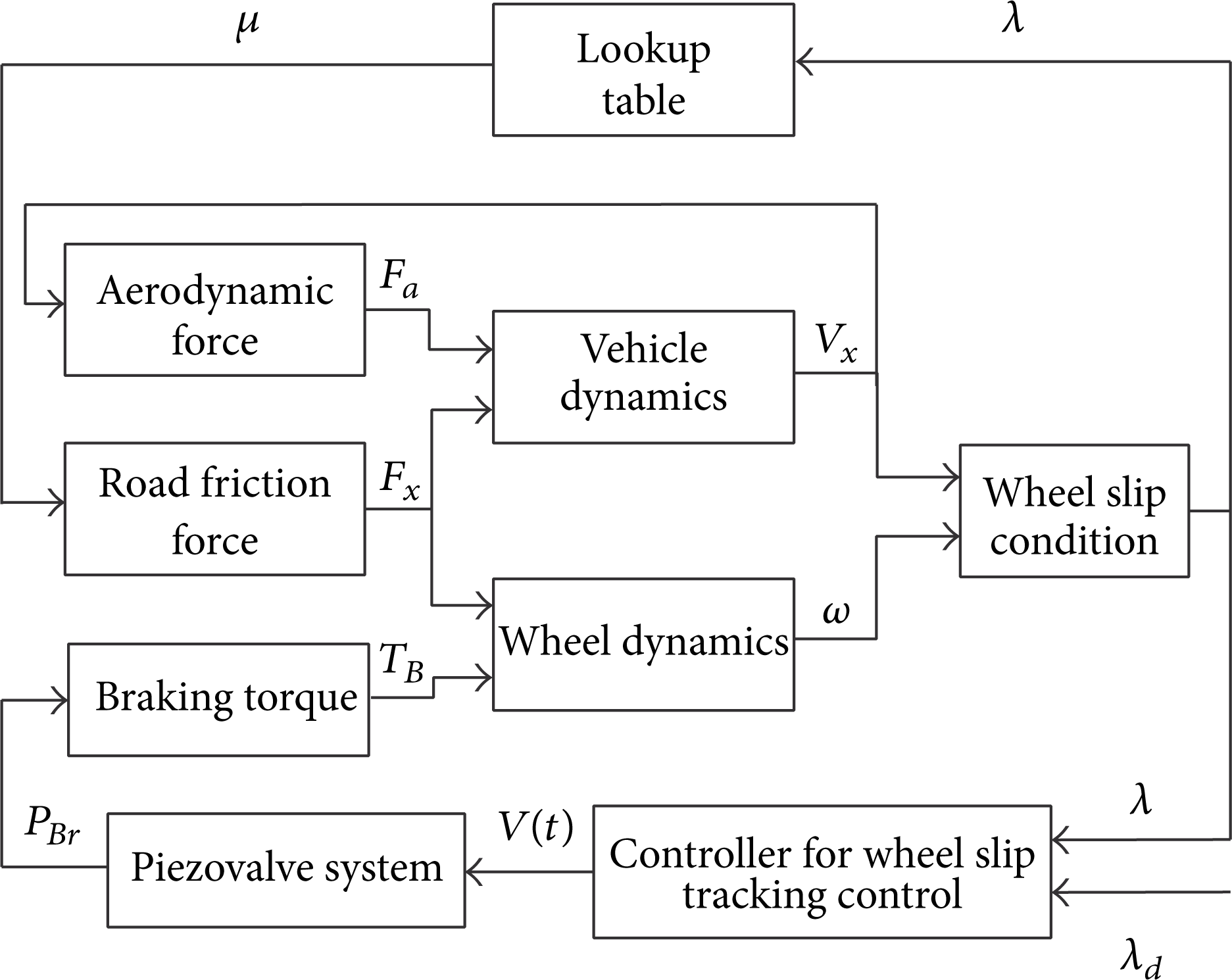
Control structure for the wheel slip control.

Figures 8 and 9 present the brake performances of the ABS featuring the piezovalve system at the dry asphalt when λ_d is set by 0.2. It is clearly observed from Figures 8(a) and 8(b) that the desired slip rate is well tracked by the controller both front and rear wheels. Thus, as shown in Figure 9, the braking distance is reduced by using the slip rate controller at various initial vehicle velocities (10 m/s, 20 m/s, and 30 m/s). The brake performance in terms of braking distance is improved by up to 1.0 m (15.9%) for 10 m/s, 4.3 m (17.1%) for 20 m/s, and 9.9 m (17.6%) for 30 m/s, respectively. Figure 8(c) presents the velocity of the vehicle and the wheel. Because the desired wheel slip is constant, the velocities of the front and the rear wheels are almost linearly decreased by the proposed braking system. Figure 8(d) shows the braking pressure of the front and rear wheels. The control input of the piezostack actuator shown in Figures 8(e) and 8(f) is less than 350 V which is suitable for the considered piezostack actuator.

Figure 8:

Braking performances: dry asphalt (λ_d = 0.2).

Figure 9:

Braking distance on dry asphalt.

On the wet asphalt condition, the brake performances are presented in Figures 10 and 11. As shown in Figures 10(a) and 10(b), the desired wheel slip rate λ_d set by 0.1 is well tracked with moderated braking pressure shown in Figure 10(d) and suitable input voltage shown in Figures 10(e) and 10(f). As already mentioned, when the desired wheel slip is around 0.1, the frictional coefficient has the highest value at wet asphalt condition. Therefore, as shown in Figure 11, the braking distance is reduced by up to 1.4 m (17.9%) for 10 m/s, 5.7 m (18.4%) for 20 m/s, and 13 m (18.7%) for 30 m/s, respectively. Because the desired wheel slip for the wet asphalt is smaller than desired wheel slip for the dry asphalt, the velocities of the wheels and vehicle are closer to each other than dry asphalt condition's results as shown in Figure 10(c).

Figure 10:

Braking performances: wet asphalt (λ_d = 0.1).

Figure 11:

Braking distance on wet asphalt.

Figure 12 presents the wheel slip rate, vehicle and wheel velocity, brake pressure, and input voltage and Figure 13 presents the comparison of the braking distance between controlled system and uncontrolled system when λ_d is set by 0.05. Figures 12(a) and 12(b) present the wheel slip of the wheel and wheel slip error, respectively. It is clearly observed that the desired wheel slip is well tracked by the proposed piezovalve system associated with the slip rate controller. As shown in Figure 12(c), because the desired wheel slip is the smallest value in this simulation, the wheel velocity is very close to the vehicle velocity. Because, as shown in Figure 5, the wet jennite condition has the smallest frictional coefficient among three conditions, braking pressure shown in Figure 12(d) is less than the braking pressure for both dry asphalt condition and wet asphalt condition. With control input of the piezostack actuator shown in Figures 12(e) and 12(f), the braking distance shown in Figure 13 is greatly reduced. The braking performance is increased by up to 6.3 m (30.7%) for 10 m/s, 25.0 m (30.8%) for 20 m/s, and 54.9 m (30.1%) for 30 m/s, respectively.

Figure 12:

Braking performances: wet jennite (λ_d = 0.05).

Figure 13:

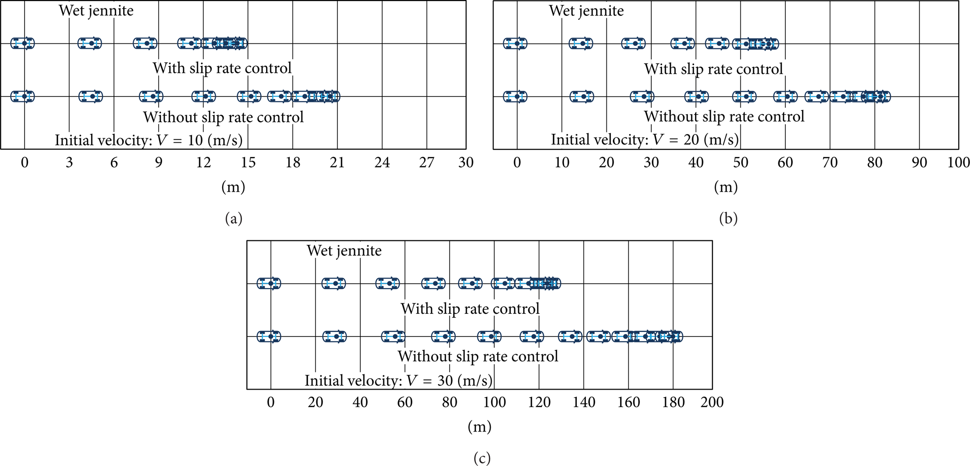
Braking distance on wet jennite.

Table 2 shows the braking distance and time at each condition with three different initial velocities. Because the frictional coefficient of the wet jennite condition is the smallest value in Figure 5, the braking distance and time are the largest results in the simulation. From the viewpoint of the braking time, the brake performances of the ABS featuring the piezovalve system are improved by around 16.6% for dry asphalt, 18.5% for wet asphalt, and 31.3% for wet jennite. This directly indicates that the proposed piezovalve system for the vehicle ABS can improve vehicle safety at different road conditions with different frictional coefficients.

Table 2:

Braking distance and time with/without slip rate controller.

Road condition	Initial velocity	Controlled		Uncontrolled
Road condition	Initial velocity	Braking distance	Braking time	Braking distance	Braking time

Dry asphalt	10 m/s	5.3 m	1.1's	6.3 m	1.3's
	20 m/s	20.8 m	2.1's	25.1 m	2.5's
	30 m/s	46.4 m	3.1's	56.3 m	3.8's

Wet asphalt	10 m/s	6.4 m	1.3's	7.8 m	1.6's
	20 m/s	25.3 m	2.5's	31.0 m	3.1's
	30 m/s	56.5 m	3.8's	69.5 m	4.6's

Wet jennite	10 m/s	14.2 m	2.8's	20.5 m	4.1's
	20 m/s	56.2 m	5.6's	81.2 m	8.2's
	30 m/s	125.1 m	8.4's	180.0 m	12.1's

5. Conclusion

In this work, a new piezoactuator-based valve system was proposed for a passenger vehicle ABS. After designing the piezovalve system, the proposed piezovalve system, longitudinal full-car dynamic model and wheel dynamic model were formulated. In order to achieve desired wheel slip rate, a sliding mode controller was then designed. Three different road conditions, dry asphalt, wet asphalt, and wet jennite, are considered and desired wheel slip rates for each condition have been well tracked by activating the proposed piezovalve system associated with the sliding mode controller. This results in the significant reducing of the stopping distance and braking time. It has been also shown that because the normal load of the front wheel is higher than the rear wheel during the braking, the braking pressure for the front wheel is higher than the rear wheel. It is finally remarked that the proposed piezovalve system is being built to undertake experimental realization as a future work.

Footnotes

Notation

Conflict of Interests

The authors declare that there is no conflict of interests regarding the publication of this paper.

References

Choi

S. B.

and Yoo

J. K.

, “Pressure control of a pneumatic valve system using a piezoceramic flapper,” Proceedings of the Institution of Mechanical Engineers C, vol. 218, no. 1, pp. 83–92, 2004.

Choi

S.-B.

Sung

K.-G.

Cho

M.-S.

, and Lee

Y.-S.

, “The braking performance of a vehicle anti-lock brake system featuring an electro-rheological valve pressure modulator,” Smart Materials and Structures, vol. 16, no. 4, article 041, pp. 1285–1297, 2007.

Choi

S.-B.

Bang

J.-H.

Cho

M.-S.

, and Lee

Y.-S.

, “Sliding mode control for anti-lock brake system of passenger vehicles featuring electrorheological valves,” Proceedings of the Institution of Mechanical Engineers D, vol. 216, no. 11, pp. 897–908, 2002.

Choi

S.-B.

Cho

M.-S.

, and Wereley

N. M.

, “Wheel-slip control of a passenger vehicle using an electrorheological valve pressure modulator,” Proceedings of the Institution of Mechanical Engineers D, vol. 220, no. 5, pp. 519–529, 2006.

Simmonds

A. J.

, “Electro-rheological valves in a hydraulic circuit,” IEE Proceedings D: Control Theory and Applications, vol. 138, no. 4, pp. 400–404, 1991.

Whittle

Firoozian

Peel

D. J.

, and Bullough

W. A.

, “Decomposition of the pressure response in an ER valve control system,” Journal of Intelligent Material Systems and Structures, vol. 5, no. 1, pp. 105–111, 1994.

Choi

S.-B.

and Sung

K.-G.

, “Control of braking force distribution using electrorheological fluid valves,” International Journal of Vehicle Design, vol. 46, no. 1, pp. 111–127, 2008.

Yoo

J.-H.

and Wereley

N. M.

, “Design of a high-efficiency magnetorheological valve,” Journal of Intelligent Material Systems and Structures, vol. 13, no. 10, pp. 679–685, 2002.

W. H.

, and Guo

N. Q.

, “Finite element analysis and simulation evaluation of a magnetorheological valve,” International Journal of Advanced Manufacturing Technology, vol. 21, no. 6, pp. 438–445, 2003.

10.

Nguyen

Q.-H.

Choi

S.-B.

, and Wereley

N. M.

, “Optimal design of magnetorheological valves via a finite element method considering control energy and a time constant,” Smart Materials and Structures, vol. 17, no. 2, Article ID 025024, pp. 1–12, 2008.

11.

Jeon

and Choi

S.-B.

, “Pressure tracking control of vehicle ABS using piezo valve modulator,” in Active and Passive Smart Structures and Integrated Systems, vol. 7977 of Proceedings of the SPIE, March 2011.

12.

Hirata

and Esashi

, “Stainless steel-based integrated mass-flow controller for reactive and corrosive gases,” Sensors and Actuators A: Physical, vol. 97–98, pp. 33–38, 2002.

13.

Tan

Hurst

, and Leo

, “Performance modeling of a piezohydraulic actuation system with active valves,” Smart Materials and Structures, vol. 14, no. 1, pp. 91–110, 2005.

14.

Jeon

Maeng

Y. J.

Choi

S. B.

Hong

S. M.

, and Lee

S. J.

, “Pressure control of a valve modulator using a piezoactuator for vehicle ABS,” in Proceedings of the 17th International Congress on Sound and Vibration, pp. 1–8, Cairo, Egypt, 2010.

15.

Kim

D. H.

and Tsao

T.-C.

, “A linearized electrohydraulic servo-valve model for valve dynamics sensitivity analysis and control system design,” Journal of Dynamic Systems, Measurement and Control, vol. 122, no. 1, pp. 179–187, 2000.

16.

W. L.

and Han

, “Piezoelectric actuator based active error compensation of precision machining,” Measurement Science and Technology, vol. 10, no. 2, pp. 106–111, 1999.

17.

Erjavec

, Automotive Brakes, TechOne, New York, NY, USA, 2004.

18.

Dukkipati

Pang

Qatu

Sheng

, and Zuo

, Road Vehicle Dynamics, SAE International, 2008.

19.

Choi

S. B.

, “Antilock brake system with a continuous wheel slip control to maximize the braking performance and the ride quality,” IEEE Transactions on Control Systems Technology, vol. 16, no. 5, pp. 996–1003, 2008.

20.

Forkenbrock

Flick

, and Garrott

, “A Comprehensive light vehicle antilock brake system test track performance evaluation,” SAE Technical Paper 1999-01-1287, 1999.

Wheel Slip Control of Vehicle ABS Using Piezoactuator-Based Valve System

Abstract

1. Introduction

2. Piezovalve System

3. Wheel Slip Control Model

4. Controller Design and Results

5. Conclusion

Footnotes

Notation

Conflict of Interests

References