Sage Journals: Discover world-class research

Abstract

As regards omnidirectional driving, conventional one- and two-pendulum spherical robots have a limited capability due to a limited pendulum motion range. In particular, such robots cannot move from a stationary state in a parallel direction to the center horizontal axis to which the pendulums are attached. Thus, to overcome the limited driving capability of one- and two-pendulum driven spherical robots, a passive version of a spherical robot, called KisBot II, was developed with a curved two-pendulum driving mechanism operated by a joystick. However, this paper presents an active upgraded version of KisBot II that includes a DSP-based control system and Task-based software architecture for driving control and data communication, respectively. A dynamic model for two-pendulum driving is derived using the Lagrange equation method, and a feedback controller for linear driving using two pendulums is then constructed based on the dynamic model. Experiments with several motions verify the driving efficiency of the proposed novel spherical robot.

1. Introduction

Most mobile robots, including those used for military, social safety, and service applications, use wheels or legs for locomotion. Yet wheeled and legged robots have several disadvantages in locomotion. Wheeled robots can be unstable and roll over; similarly legged robots can fall over in certain terrains, making the robots immobile. Furthermore, protecting the electronic components from the external environment can be difficult with such mobile robots.

Thus, to overcome the structural weaknesses of conventional mobile robots, various studies have investigated the feasibility of spherical robots. When compared with wheeled and legged robots, spherical robots have several advantages, including no chance of rolling over due to their symmetrical structure, the capacity of omnidirectional driving, no problem with obstacles, inner component protection from the external environment, such as liquid, dust, and gas, and a high energy efficiency due to single contact point with the ground [1].

However, in terms of obstacle avoidance, slope climbing, balance control, and driving control, wheeled and legged robots are currently still superior to spherical robots. This is because a spherical robot is a nonholonomic system. However, spherical robots are still in the initial stage of development, and research on their mechanical structure and driving mechanism is receiving serious attention due to the various advantages mentioned above. In terms of locomotion, the driving mechanism is the most key factor, and there are currently five main types of driving mechanism for spherical robots according to the driving system structure. The first is the single-wheel type, where Halme et al. introduced a spherical robot with an IDU (inside driving unit) consisting of a driving wheel and balance wheel [2]. The second is the car type, where Bicchi et al. developed the spherical that is driven by a car inside the sphere [3]. The third is the internal weight type, where Javadi and Mojabi developed a spherical robot that moves by changing the center of mass for the outer shell using four movable weights located inside the shell [4]. The fourth is the attached rotor type, where Bhattacharya and Agrawal developed a tow rotor-driven spherical robot [5]. And finally, the fifth is the pendulum type, which is subdivided into the one-pendulum type [6 –10] and two-pendulum type [11 –13]. In addition to these five main types of driving mechanism, various other driving mechanisms have also been studied for spherical robots [14 –16].

However, each type of driving mechanism has disadvantages. In the case of the single-wheel type, there are problems with stable steering and balance control. For the car type, there is a chance of noncontact between the inside of the outer shell and the car wheel, creating an uncontrollable status. Meanwhile, fast steering is difficult for the internal weight type and attached rotor type, whereas the pendulum type, including both the one- and two-pendulum types, lacks omnidirectional movement due to pendulum movement limitations. Plus, the two-pendulum type has a balance control problem.

The current authors have already studied and developed a series of spherical robots, called KisBot (Kyungpook national university Intelligent Spherical robot). Based on KisBot I, which was driven in a wheeling mode and rolling mode using two pendulums, a new driving mechanism was developed to improve the driving capability of a two-pendulum driven spherical robot. Accordingly, this paper presents an active version of KisBot II that includes a novel curved two-pendulum driving system and improved driving capability. When compared with the conventional one-pendulum or two-pendulum spherical robot, KisBot II has an improved movement direction capability from a stationary state, omnidirectional driving capability using a base frame operation for two-pendulum driving, and the capability to change the driving direction by adding a rotational degree of freedom to the pendulum in parallel with the horizontal axis. The initial studies of the passive version of KisBot II operated by a joystick were introduced at the 15th IEEE international conference on intelligent engineering systems (INES 2011) held in June 2011 in Slovakia [17].

Since then, KisBot II has been upgraded to an active version that includes improvements to the control hardware, software, and outer shell. The design details of the driving mechanism and system description of the active version of KisBot II are described in Section 2. Section 3 explains the dynamic equation used for linear motion based on the Lagrange method. Section 4 presents the simulations and experiments using linear driving motion control with pendulum rotation, plus some other experiments for additional motion generation. A nonlinear feedback controller with a computed torque concept is constructed for the linear driving motion. The experiment results confirm the driving efficiency, and some final conclusions including future work are also provided.

2. Driving Mechanism and System Description of KisBot II

2.1. Design Concept

The general movement paths of a pendulum inside a pendulum-driven spherical robot are shown in Figure 1.

Figure 1:

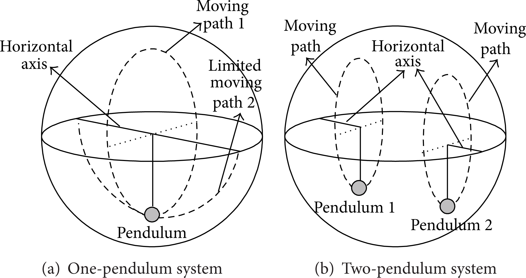
Pendulum movement paths of conventional pendulum driven spherical robots.

In the case of a one-pendulum driven robot where the pendulum is located at its center, there are two movement paths for the pendulum, as shown in Figure 1(a). Path 1 is generated by rotation of the horizontal center axis, and path 2 is generated by rotation of the pendulum. While path 1, which is orthogonal to the horizontal axis, has an unlimited motion range, path 2, which is parallel with the horizontal axis, has a limited motion range as the pendulum and horizontal axis belong to the same plane. As a result, a one-pendulum spherical robot has a limited driving direction capacity.

The two-pendulum system structure is shown in Figure 1(b). While each movement path of the pendulums is orthogonal to the horizontal axis to which each pendulum is attached, it is hard to generate a movement path parallel with the horizontal axis, like path 2 for the one-pendulum structure. Even if such path was generated, as in Figure 1(a), the movement range of the pendulum would still be limited for the same reason as explained for path 2 in Figure 1(a).

Consequently, changing the driving direction orthogonally and steering while moving are both difficult for a two-pendulum driven spherical robot. To overcome such problems, an adjustable length for the horizontal axis was introduced using a linear actuator structure; yet this causes balance control difficulties.

Figure 2 shows that the proposed two-pendulum structure does not have any movement range limitations for the pendulums inside the sphere. Figure 2(a) shows the movement paths of the two pendulums around the horizontal axis, the same as path 1 in Figure 1(a). Each pendulum can also rotate independently without any interference with the horizontal axis, as shown in Figure 2(b).

Figure 2:

Pendulum movement paths of KisBot II.

Thus, the proposed hybrid pendulum driving mechanism includes the features of both a one-pendulum and two-pendulum driving mechanism.

2.2. Motion Generation

Figure 3 shows a comparison of the driving directions from stationary state between a conventional pendulum driven spherical robot and the proposed hybrid pendulum driven spherical robot.

Figure 3:

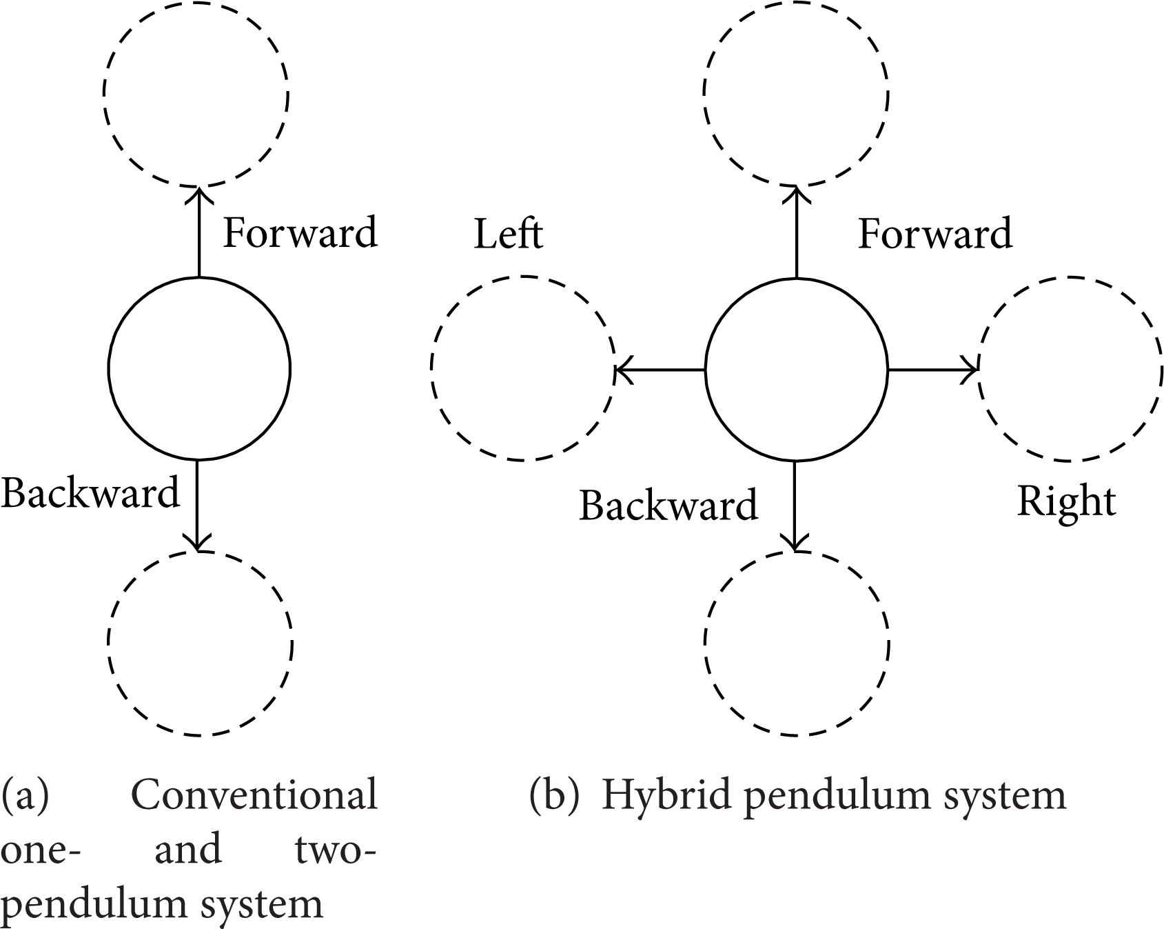
Comparison of driving directions from stationary state.

From a stationary state, the conventional one- and two-pendulum driving mechanism for a spherical robot has two driving directions, forward/backward, whereas the proposed hybrid pendulum driving mechanism has four driving directions, forward/backward/right/left.

When changing the driving direction, the conventional one-pendulum spherical robot can steer its driving direction with a certain radius of a curvature path, as shown in Figure 4(a), while the conventional two-pendulum spherical robot has almost no steering control of its driving direction. However, the proposed hybrid pendulum spherical robot can steer its driving direction like a one-pendulum spherical robot and change its driving direction orthogonally while moving, as shown in Figure 4(b).

Figure 4:

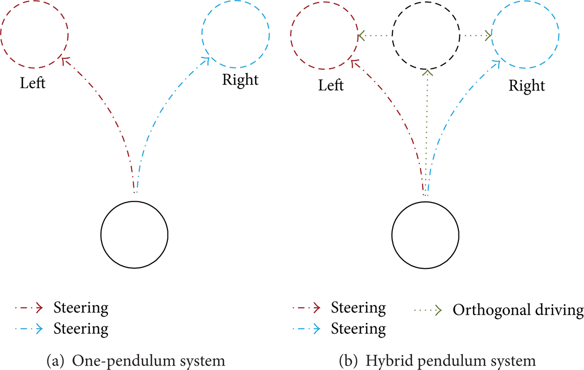
Comparison of changing driving direction.

Thus, the proposed driving mechanism can provide an improved locomotion capacity for a spherical robot when compared to the conventional one-pendulum and two-pendulum spherical robot.

Figure 5 shows a comparison of the pendulum movement range between the conventional one-pendulum driven spherical robot and the proposed hybrid pendulum driven spherical robot, KisBot II. For KisBot II, the driving mechanism using base frame rotation is the same as that for the conventional one-pendulum.

Figure 5:

Comparison of pendulum movement range between one-pendulum system and hybrid pendulum system as regards steering.

Furthermore, if the horizontal axis can be made to stand vertically, the proposed robot can move in any direction by pendulum rotation according to the rotation angle of the horizontal axis, as shown in Figure 6.

Figure 6:

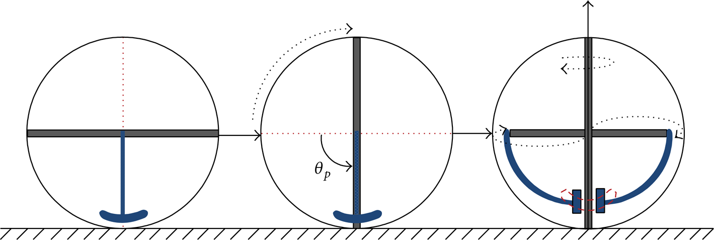
Base frame rotation for changing driving direction.

2.3. Mechanical System Structure

2.3.1. Basic Structure and Motion Principles

The basic mechanical structure of KisBot II consists of a horizontal ring frame and vertical ring frame. At the center of the robot, there is a cross-shaped frame, called the base frame, which is also connected to the horizontal ring frame. The pendulum rod is curve-shaped.

The base frame generates the pendulum movement path, as shown in Figure 2(a), and the pendulums are designed to rotate without any interference with the main shaft of the base frame to generate the movement paths shown in Figure 2(b).

The sustained operations of the base frame rotation and pendulum rotation are also shown in Figures 7 and 8, respectively, along with the whole mechanical structure designed by CATIA. More detailed descriptions of the mechanical structure are provided in [17].

Figure 7:

Motion principle of base frame.

Figure 8:

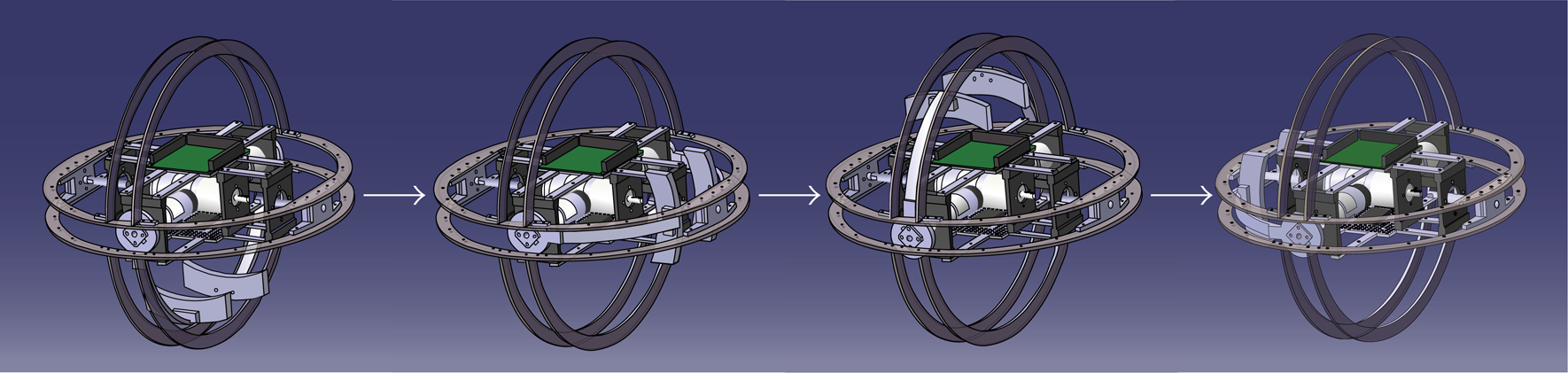
Motion principle of pendulum.

2.3.2. Redesigned Outer Shell

The original outer shell of KisBot II consisted of eight parts. Yet this created assembly problems, as the outer shells were connected to the mechanical ring frames with internal bolts, plus inconsistencies resulted in an uneven surface for the robot. Thus, to improve the assembly and consistency, the outer shell was redesigned with four parts and holes for the bolts on the surface of the shell, as shown in Figure 9.

Figure 9:

Drawings of redesigned outer shell.

To sustain external impact, the thickness of the shell was increased from 2 mm to 4 mm and made of polyamide instead of resin using a rapid prototype process. Figure 10 shows the manufactured outer shell. When fully assembled, the radius of the improved KisBot II was about 17.2 cm, an increase of 0.7 cm. Urethane coating was also applied to the surface of the shell for protection and to prevent slipping on the ground.

Figure 10:

Manufactured outer shell.

2.4. Control System Structure

2.4.1. System Hardware

DSP320F2812 is applied to the proposed spherical robot as the main processor. For motor control, the main processor generates PWM (pulse width modulation) signals for the base frame dc motor and pendulum motors. Each PWM signal is then transferred to the motor driver board, which outputs a switching voltage matched with 22.4 V for the base frame and pendulum dc motor operation. An encoder attached to each pendulum dc motor outputs the motor shaft position information. Two QEPs (quadrature encoder pulse) within the DSP are used to count the encoder output values for each pendulum motor. Meanwhile, the encoder value for the base frame dc motor is counted using an external counter chip.

KisBot II uses a Bluetooth protocol to communicate with a PC that has a GUI (graphic user interface). The PC transfers data, such as driving and stop commands, to KisBot II, while the robot transfers the robot status data, including the driving velocity, motor encoder values, and sensor data, to the PC. An AHRS (attitude heading reference system) is also applied to the current version of KisBot II. The control system architecture is shown in Figure 11.

Figure 11:

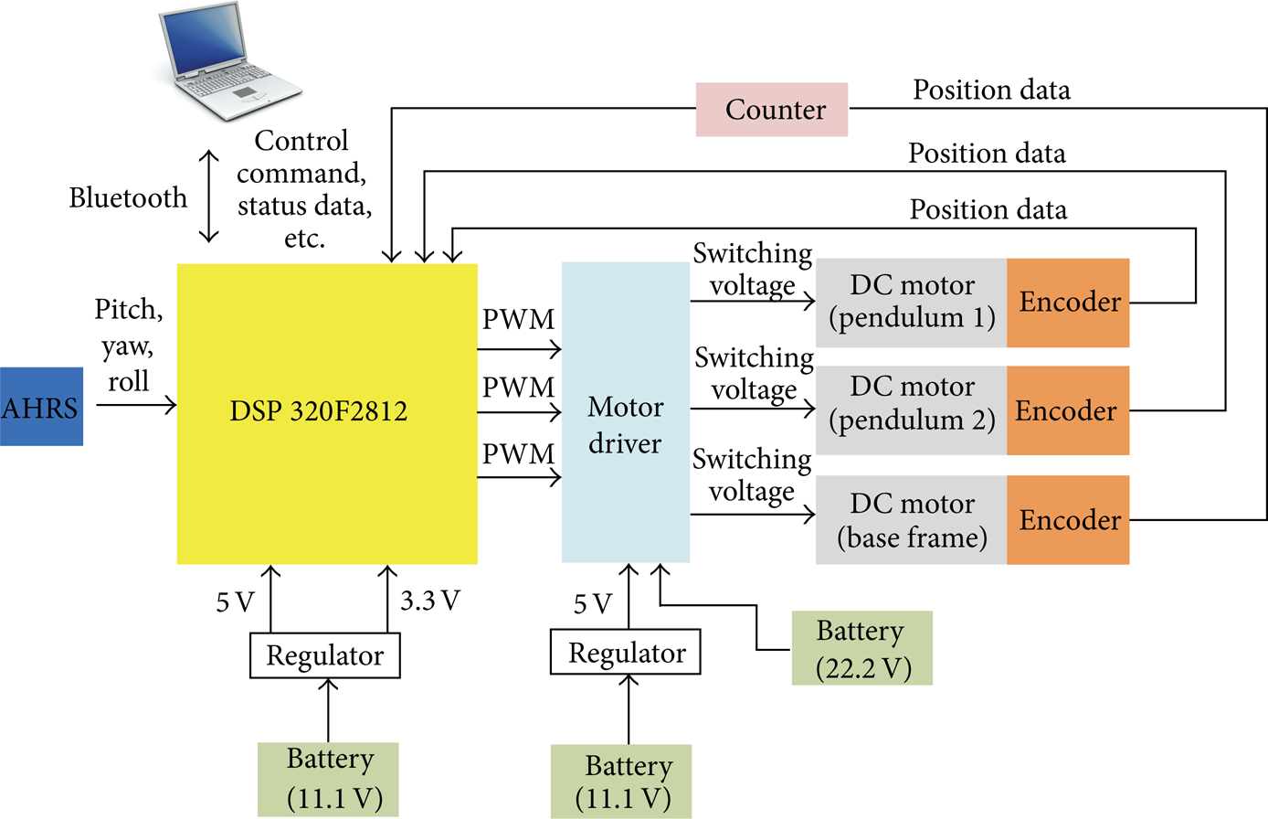
Block diagram of control system.

The entire implemented control system and its component configuration, including the control boards, wire harness, motors, and batteries, are shown in Figure 12.

Figure 12:

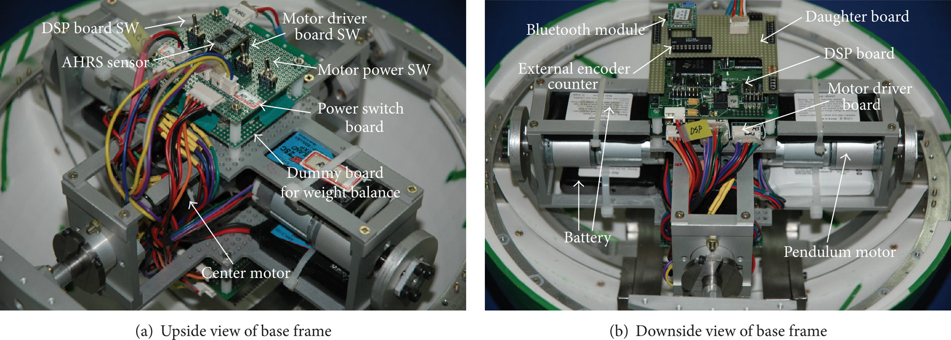
Implemented control system and component configuration.

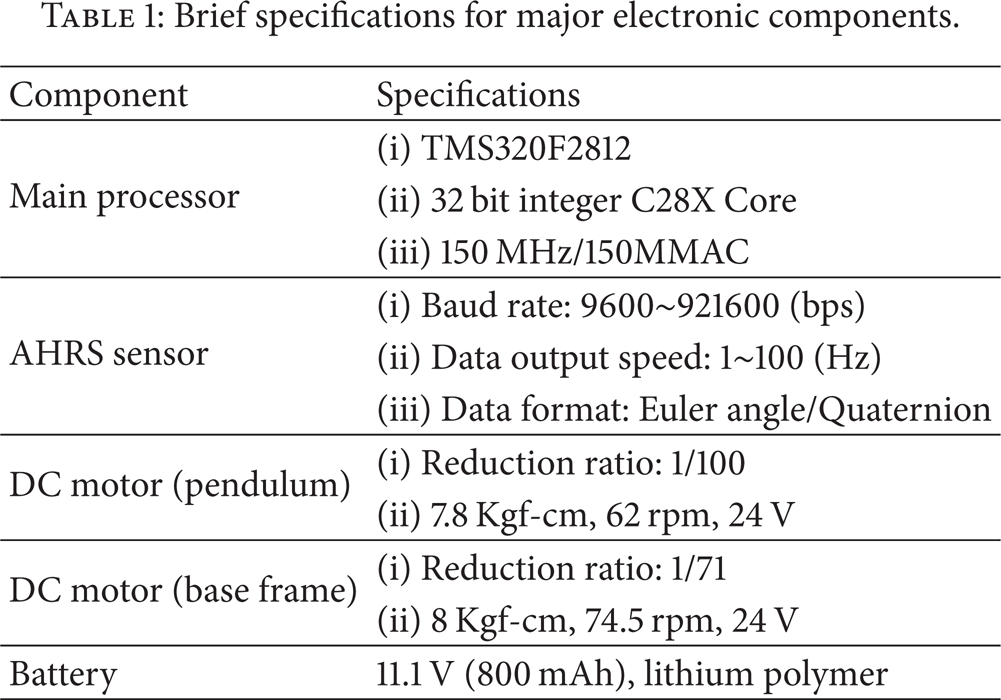
The motor for the base frame rotation is located inside the base frame and four batteries with the same weight are located above and below each pendulum motor to balance the weight of the base frame. The power switch board is attached to the upper center of the base frame. Meanwhile, the motor driver board, DSP board, and daughter board for the Bluetooth and external encoder counter are placed in order at the lower center of the base frame. The major electronic components are shown in Table 1.

Table 1:

Brief specifications for major electronic components.

Component	Specifications

Main processor	(i) TMS320F2812
	(ii) 32 bit integer C28X Core
	(iii) 150 MHz/150MMAC

AHRS sensor	(i) Baud rate: 9600∼921600 (bps)
	(ii) Data output speed: 1∼100 (Hz)
	(iii) Data format: Euler angle/Quaternion

DC motor (pendulum)	(i) Reduction ratio: 1/100
DC motor (pendulum)	(ii) 7.8 Kgf-cm, 62 rpm, 24 V

DC motor (base frame)	(i) Reduction ratio: 1/71
DC motor (base frame)	(ii) 8 Kgf-cm, 74.5 rpm, 24 V

Battery	11.1 V (800 mAh), lithium polymer

2.4.2. System Software

The control software of KisBot II consists of two interrupt service routines, SCI A and SCI B. The data communications between the robot and the external PC are accomplished through the SCI A interrupt service routine, while the robot receives the data from the AHRS with a 20 msec time period through the SCI B interrupt service routine.

The main robot control routine that controls the motors for the robot driving and various robot status data is located within SCI B for timing control. Figure 13 shows the control software flowchart for KisBot II.

Figure 13:

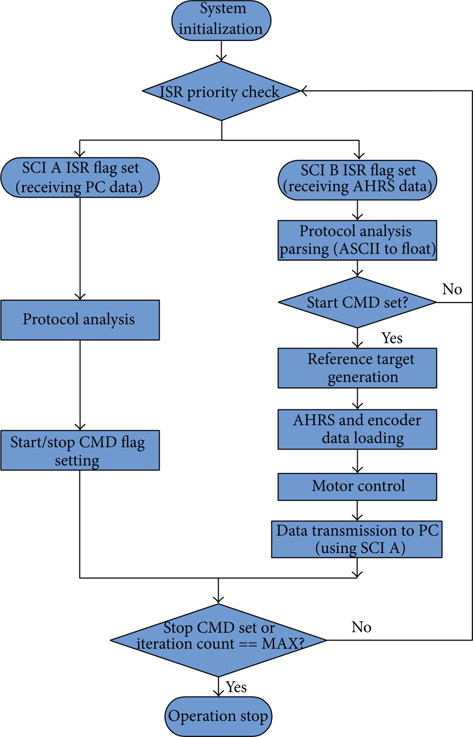
Control software flow chart.

3. Motion Control for Linear Motion

3.1. Dynamic Model

Linear motion equations can be derived mathematically by using Newton's Law of motion and the Lagrange method based on the assumptions for the motion equation simplification that there is no slip between the shell of the robot and the floor and no robot rotational torque loss by the frictional torque between the robot and the floor [7]. KisBot II has two linear motions using two-pendulum rotation and base frame rotation. However, the main linear driving of the proposed robot is performed using two-pendulum rotation. Therefore, this paper focuses on the mathematical dynamic model for pendulum driven linear motion.

While the base frame is motor weight symmetric for pendulum rotation, it is not motor weight symmetric for base frame rotation due to the position and weight distribution of the motors. Thus, in the case of pendulum driving, KisBot II can be modeled as a sphere with an unbalanced rod weight at its center. The simplified model is shown in Figure 14.

Figure 14:

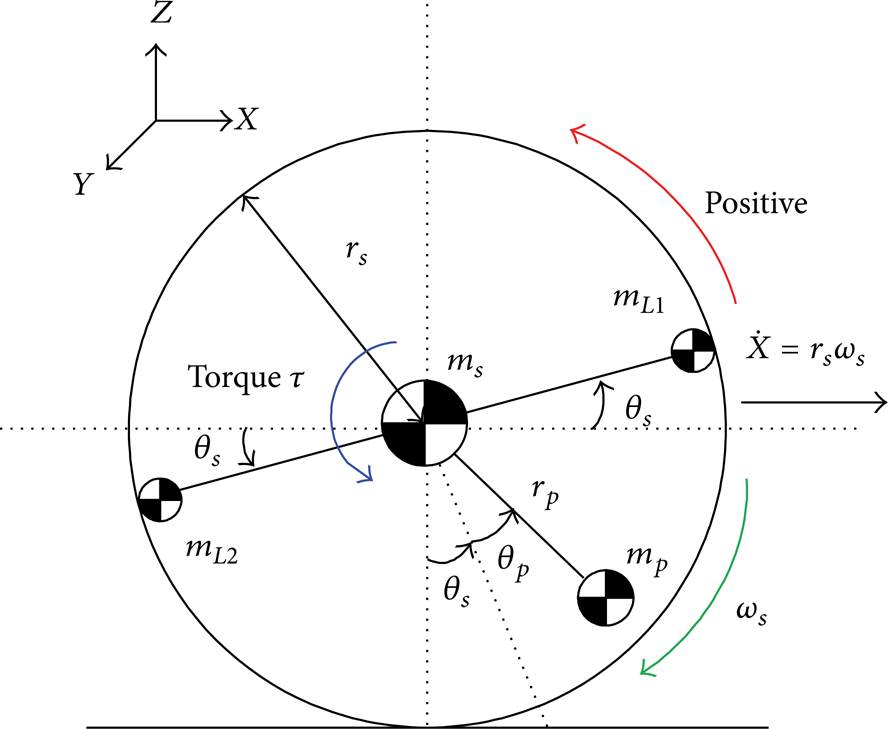
Simplified model of pendulum driving motion.

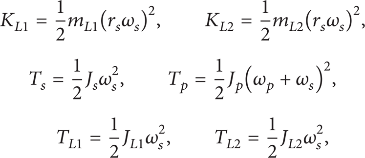
The potential energy, kinetic energy, and rotational energy for both the sphere and pendulum are given as follows:

\begin{matrix} U_{s} = 0, U_{p} = m_{p} g (r_{s} - r_{p} \cos (θ_{p} + θ_{s})), \\ U_{L 1} = m_{L 1} g r_{s} (1 + \sin θ_{s}), \\ U_{L 2} = m_{L 2} g r_{s} (1 - \sin θ_{s}), \\ K_{s} = \frac{1}{2} m_{s} {(r_{s} ω_{s})}^{2}, \\ K_{p} = \frac{1}{2} m_{p} \{{(r_{s} ω_{s} - r_{p} \cos (θ_{p} + θ_{s}) (ω_{p} + ω_{s}))}^{2}) (+ {(r_{p} \sin (θ_{p} + θ_{s}) (ω_{p} + ω_{s}))}^{2}\}, \\ K_{L 1} = \frac{1}{2} m_{L 1} {(r_{s} ω_{s})}^{2}, K_{L 2} = \frac{1}{2} m_{L 2} {(r_{s} ω_{s})}^{2}, \\ T_{s} = \frac{1}{2} J_{s} ω_{s}^{2}, T_{p} = \frac{1}{2} J_{p} {(ω_{p} + ω_{s})}^{2}, \\ T_{L 1} = \frac{1}{2} J_{L 1} ω_{s}^{2}, T_{L 2} = \frac{1}{2} J_{L 2} ω_{s}^{2}, \end{matrix}

(1)

where, $J_{s} = (2 / 3) m_{s} r_{s}^{2}$ , J_p = m_pr_p², J_L1 = m_L1r_s², and J_L2 = m_L2r_s².

U_s, U_p: potential energy of sphere and pendulum.

U_L1, U_L2: potential energy for each mass in center rod.

K_s, K_p: kinetic energy of sphere and pendulum.

K_L1, K_L2: kinetic energy for each mass in center rod.

T_s, T_p: rotational energy of sphere and pendulum.

T_L1, T_L2: rotational energy for each mass in center rod.

m_s, m_p: mass of sphere and pendulum.

m_L1, m_L2: each mass in center rod.

r_s: radius of sphere.

r_p: length of pendulum rod.

θ_s, θ_p: rotation angle of sphere and pendulum.

ω_s, ω_p: angular velocity of sphere and pendulum.

J_s, J_p: moment of inertia of sphere and pendulum.

J_L1, J_L2: moment of inertia for each mass in center rod.

g: acceleration of gravity.

Here, the Lagrange function can be defined as follows:

\begin{array}{l} L = K_{total} + T_{total} - U_{total} \\ = K_{s} + K_{p} + K_{L 1} + K_{L 2} + T_{s} + T_{p} + T_{L 1} + T_{L 2} - U_{s} - U_{p} - U_{L 1} - U_{L 2} . \end{array}

(2)

The Lagrange equations of motion are then derived as follows:

\begin{matrix} \frac{d}{d t} (\frac{L}{\partial ω_{s}}) - \frac{\partial L}{\partial θ_{s}} = - τ + τ_{f} \\ \frac{d}{d t} (\frac{L}{\partial ω_{p}}) - \frac{\partial L}{\partial θ_{p}} = τ, \end{matrix}

(3)

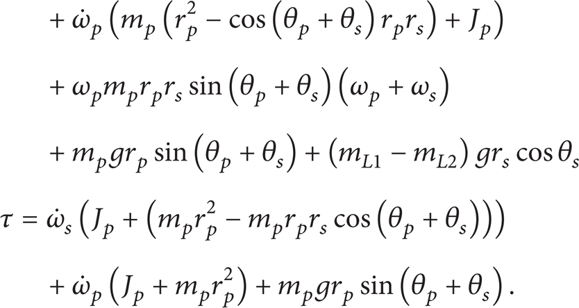
where t represents time, τ means the torque of the pendulum dc motor, and τ_f means the torque generated by the friction between the sphere and the floor. Here, τ_f is ignored for the motion equation simplification as it is assumed that the robot rolls on the floor without slipping and has no torque loss by the frictional torque. According to (3), the dynamic equations can be written as (4) and (5), respectively:

- τ = {\dot{ω}}_{s} (J_{L 1} + J_{L 2} + J_{s} + J_{p}) + m_{p} (r_{p}^{2} - 2 \cos (θ_{p} + θ_{s}) r_{p} r_{s} + r_{s}^{2}) (+ r_{s}^{2} (m_{L 1} + m_{L 2} + m_{s})) + ω_{s} m_{p} r_{p} r_{s} \sin (θ_{p} + θ_{s}) (ω_{p} + ω_{s}) + {\dot{ω}}_{p} (m_{p} (r_{p}^{2} - \cos (θ_{p} + θ_{s}) r_{p} r_{s}) + J_{p}) + ω_{p} m_{p} r_{p} r_{s} \sin (θ_{p} + θ_{s}) (ω_{p} + ω_{s}) + m_{p} g r_{p} \sin (θ_{p} + θ_{s}) + (m_{L 1} - m_{L 2}) g r_{s} \cos θ_{s}

(4)

While these dynamic equations are not integrable, they provide the basis for constructing the linear motion controller. θ_p + θ_s, called the driving angle, means the tilting angle of the pendulum relative to the vertical reference line in a global coordinate system.

3.2. Feedback Controller Design

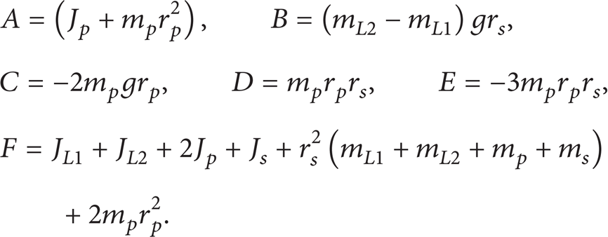
When developing a dynamic equation for a pendulum driven spherical robot, the trigonometric functions in the dynamic equation are usually linearized on the assumption that the driving angle is almost zero. Thereafter, a Laplace transform is applied to the linearization of the dynamic function to construct the PID controller [7, 9, 18]. However, linearization is not suitable for the proposed system due to the cos⁡θ_s term in (4) caused by the unequal weight balance of the center rod. Thus, linearization of the trigonometric functions could not be applied to the present dynamic model for designing the controller. Therefore, the speed controller for linear motion was designed using a nonlinear dynamic equation based on a computed torque method concept. Using (4) and (5), the nonlinear dynamic equation is expressed as follows:

τ = {\dot{ω}}_{s} (J_{p} + (m_{p} r_{p}^{2} - m_{p} r_{p} r_{s} \cos (θ_{p} + θ_{s}))) + {\dot{ω}}_{p} (J_{p} + m_{p} r_{p}^{2}) + m_{p} g r_{p} \sin (θ_{p} + θ_{s}) .

(5)

where,

{\dot{ω}}_{s} = (A {\dot{ω}}_{p} + B \cos θ_{s} + (C + D {\dot{ω}}_{p} - D {(ω_{p} + ω_{s})}^{2})) (\times \sin (θ_{p} + θ_{s})) \times {(E \cos (θ_{p} + θ_{s}) + F)}^{- 1},

(6)

The simplified first order DC motor model for the input voltage and pendulum rotation velocity, while neglecting the internal inductance, can be written as follows:

\begin{matrix} A = (J_{p} + m_{p} r_{p}^{2}), B = (m_{L 2} - m_{L 1}) g r_{s}, \\ C = - 2 m_{p} g r_{p}, D = m_{p} r_{p} r_{s}, E = - 3 m_{p} r_{p} r_{s}, \\ F = J_{L 1} + J_{L 2} + 2 J_{p} + J_{s} + r_{s}^{2} (m_{L 1} + m_{L 2} + m_{p} + m_{s}) + 2 m_{p} r_{p}^{2} . \end{matrix}

(7)

where $a = n K_{t} / R_{m}$ , $b = (K_{t} K_{e} / R_{m}) + f_{m}$ , and J = J_m + n²J_p.

J_m, n, K_t, K_e, R_m, and f_m mean the moment of inertia of the motor shaft, gear ratio, torque constant, back EMF constant, resistance of the motor, and viscous friction coefficient, respectively. Substituting (8) for (6) yields

{\dot{ω}}_{p} = \frac{a}{J} V - \frac{b}{J} ω_{p},

(8)

If the driving angle, θ_p + θ_s, is controlled at 0 while the robot is moving, sin(θ_p + θ_s) is approximately 0 and cos⁡(θ_p + θ_s) is approximately 1 in (9). The angular acceleration of the sphere, ${\dot{ω}}_{s}$ , can then be regarded as

{\dot{ω}}_{s} = \frac{A ((a / J) V - (b / J) ω_{p}) + B \cos θ_{s}}{E \cos (θ_{p} + θ_{s}) + F} + ((C + D \times A ((a / J) V - (b / J) ω_{p}) - D {(ω_{p} + ω_{s})}^{2})) (\times \sin (θ_{p} + θ_{s})) {\times (E \cos (θ_{p} + θ_{s}) + F)}^{- 1} .

(9)

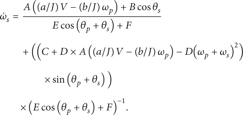
where $\tilde{A} = a A / J (E + F)$ , $\tilde{B} = b A / J (E + F)$ , and $\tilde{C} = B / (E + F)$ .

If the control input to the pendulum motor is designed such that $u_{inner} = K_{2} \tilde{B} ω_{p} - K_{3} \tilde{C} \cos θ_{s}$ to cancel the second and third terms of (10), (10) can be regarded as follows:

{\dot{ω}}_{s} \approx \tilde{A} V - \tilde{B} ω_{p} + \tilde{C} \cos θ_{s},

(10)

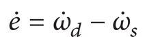
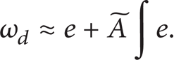
The error for the reference velocity can be defined as (12) and (13). Substituting (13) for (11) and integration of the resulting equation yields (14). Consider

{\dot{ω}}_{s} \approx \tilde{A} V .

(11)

As the input voltage of the DC motor for the pendulum rotation is decided by the error between the reference velocity and the real velocity, (14) can be rewritten as (15). This means that the velocity control of the robot to follow the reference velocity can be performed using a linear feedback controller for the DC motor, such as a PI controller with nonlinear term cancellations

e = ω_{d} - ω_{s}

(12)

As a result, the entire control input to the DC motor of the pendulum to produce the reference velocity as real output consists of the input from the linear feedback controller, input to make the driving angle zero, and input to compensate the nonlinear terms in the robot acceleration, as shown in

\dot{e} = {\dot{ω}}_{d} - {\dot{ω}}_{s}

(13)

Using these procedures, a nonlinear feedback speed controller was constructed, as shown in Figure 15.

Figure 15:

Nonlinear feedback controller for linear driving motion.

In Figure 15, the angular velocity follow-up control for the reference velocity profile is achieved using a PID controller in the first feedback loop, while the compensation control to make driving angle zero is achieved in the second feedback loop. This second feedback loop is equivalent to a control loop in which the driving angle reference is set to zero and the reference driving angle follow-up control is performed by proportional control. The third and last feedback loop carries out the nonlinear compensation for the second and third terms in (10).

4. Experimental Results

4.1. Linear Velocity Control in Pendulum Rotation Driving

Simulations using MATLAB Simulink were conducted to verify the efficiency of the proposed velocity controller. (6) was used as the plant. The mechanical parameters of the proposed system used in the simulations were measured and are shown in Table 2.

Table 2:

Mechanical parameters of KisBot II.

Symbols	Values

r_s	0.172 m
r_p	0.12 m
m_s	3.3480 Kg
m_p	1.28 Kg
m_L = m_L1 + m_L2	1.1560 Kg
J _s	0.066 Kgm²
J _p	0.0184 Kgm²

The DC motor model of the pendulum used in simulations is given as (17). It was modeled based on the specification data provided by the manufacturer. Consider

ω_{d} \approx e + \tilde{A} \int V .

(14)

ω_{d} \approx e + \tilde{A} \int e .

(15)

ω_{d} = U (u_{PID} + u_{D A = 0} + u_{inner}) .

(16)

\frac{ω_{p} (s)}{V (s)} = \frac{0.118}{0.009216 s + 0.037924} .

(17)

The driving velocity simulation results are shown in Figure 16. 120 deg/s was used as the reference velocity. Kp = 0.05, Ki = 1.2, and Kd = 0.012 were used as the PID controller gain, K1 = −1.5 as the driving angle feedback gain, K2 = 0.009 as the pendulum angular velocity feedback gain, and K3 = 0.01 as the sphere angle feedback gain. All of the gains were experimentally tuned. To investigate the influence of the center rod weight imbalance on the robot driving velocity, simulations were conducted for cases with different weight ratios between m_L1 and m_L2, plus the same weight ratio.

Figure 16:

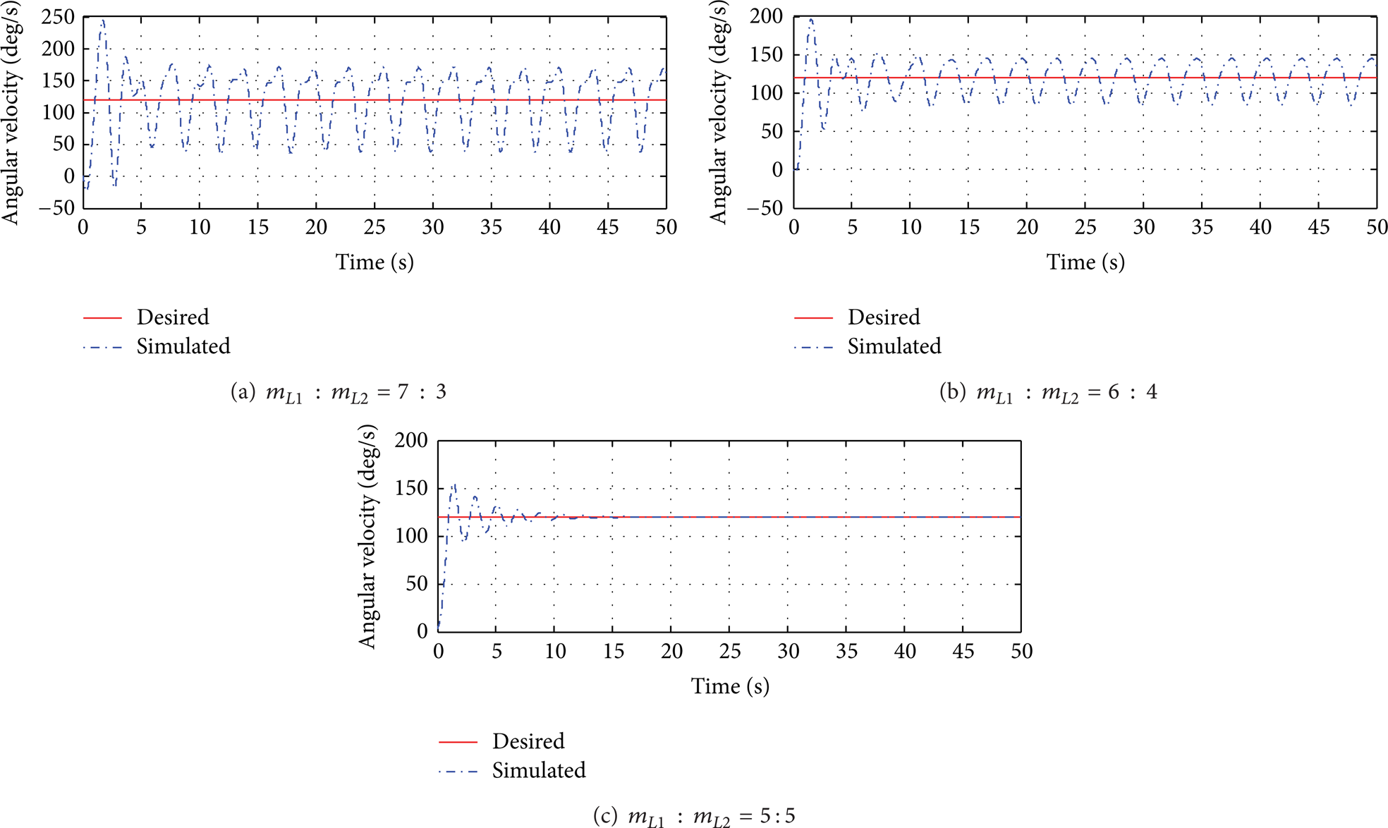
Step response simulation results according to ratio between m_L1 and m_L2.

As shown in Figure 16, when the weight imbalance of the center rod was lower, less oscillation was produced in the driving velocity output. Thus, the simulation results inferred that the cos⁡θ_s term of (6) resulting from the center rod weight imbalance created oscillation during the robot driving. Thus, if the weight of the center rod could be evenly balanced, the oscillation in the driving velocity could be reduced or even eliminated.

Before the linear velocity control experiment, a constant voltage input (8 V) was applied to the pendulum motors to investigate the characteristic of the robot driving velocity in the case of a constant pendulum rotation. The results are shown in Figure 17.

Figure 17:

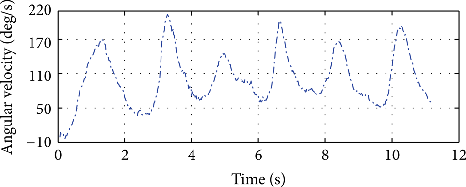
Robot angular velocity with 8 V input to pendulum motors.

Despite an almost constant pendulum rotation, there were still oscillations in the robot velocity. From this experimental result and the simulation results of Figure 16, it is possible to deduce that the test robot has a mechanical weight imbalance in the center rod where the center motor is placed for the base frame rotation.

A velocity control experiment was performed using the implemented nonlinear feedback controller in a real system. The reference robot angular velocity profile consisted of exponentially increasing velocity (from 0 deg/s to 120 deg/s) section, constant speed (120 deg/s) section, and exponentially decreasing velocity (from 120 deg/s to 0 deg/s) section, respectively. The reference velocity tracking control results and robot moving position results according to its velocity are shown in Figures 18 and 19, respectively.

Figure 18:

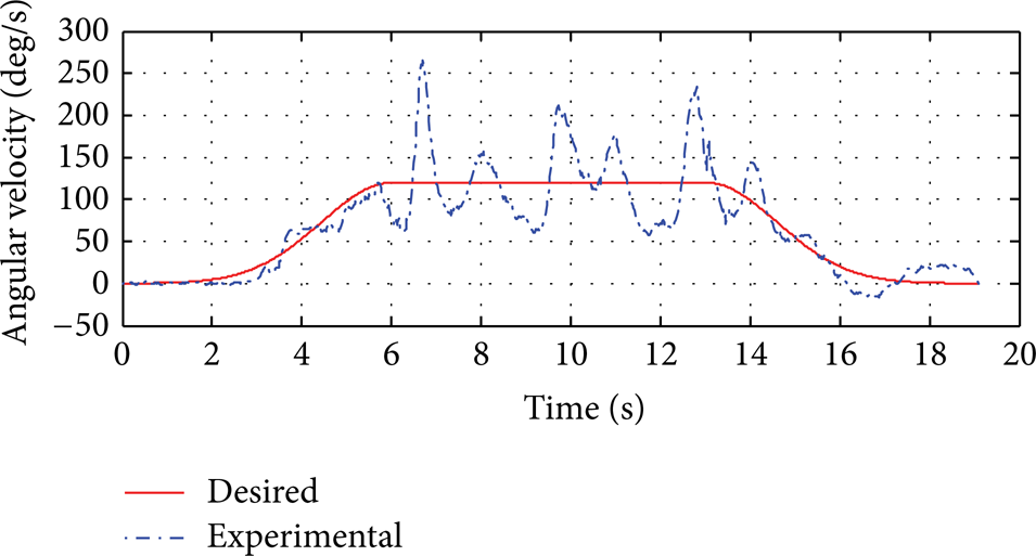
Reference velocity tracking control results.

Figure 19:

Moving position results.

Kp = 0.059, Ki = 1.17, Kd = 0.014, K1 = −1.29, K2 = 0.012, and K3 = 0.012 were all used in the real system and tuned experimentally, as in the simulation based on the simulation gains. Oscillations were recorded in the constant speed section and presumed to be the effect of the weight imbalance of the center rod of the base frame. Notwithstanding, the robot was still essentially able to follow the reference velocity. As regards the linear moving position, KisBot II moved linearly with a small yet reasonable error for the reference position, as shown in Figure 19.

Thus, based on the above results, even though the proposed controller design method is somewhat intuitive, the nonlinearities could be reduced to a reasonable level during the robot driving. Therefore, the simulations and real experiments verified the efficiency of the constructed controller for the proposed system. Although not shown in this paper, when using a PID controller alone, the robot was uncontrollable as regards velocity control.

4.2. Other Motion Generation

The driving motion in the case of simultaneous rotation of both the pendulum and the base frame is presented in Figure 20. When compared to the case of increasing yet limiting the pendulum tilting angle in [18], the proposed unique pendulum operation allowed the creation of interesting trajectories, as shown below, including spirals and the 8-figure trajectories in [18].

Figure 20:

Snapshots of driving motion by both pendulum and base frame rotation.

Figure 21 shows the change in the driving direction of KisBot II when maintaining the rotation angle of the base frame vertical to the ground. The driving directions of the robot according to the angle of the base frame from the center line are shown in Figures 21(a)–21(d).

Figure 21:

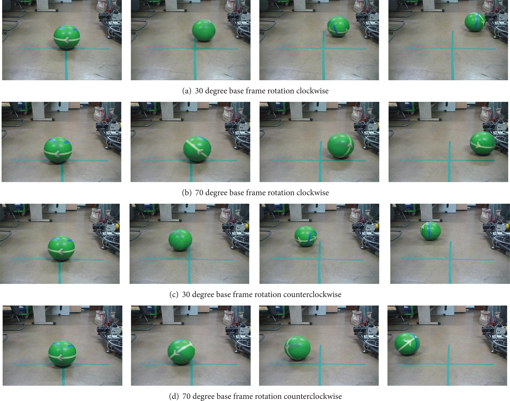
Driving direction according to rotation angle of base frame.

As mentioned in Section 2, the base frame can be rotated by the motor located in the center rod within the robot without making the outer shell rotate. Due to this mechanism, the driving direction of the robot can be decided by the rotation angle of the base frame. Thereafter, the robot can drive in any direction using pendulum rotation, as shown in Figure 21.

These results mean that KisBot II has an omnidirectional driving ability in the case of driving using pendulum rotation.

The experimental results of orthogonal driving for obstacle avoidance on the assumption that the robot will meet obstacles, such as a wall or valley, are shown in Figure 22.

Figure 22:

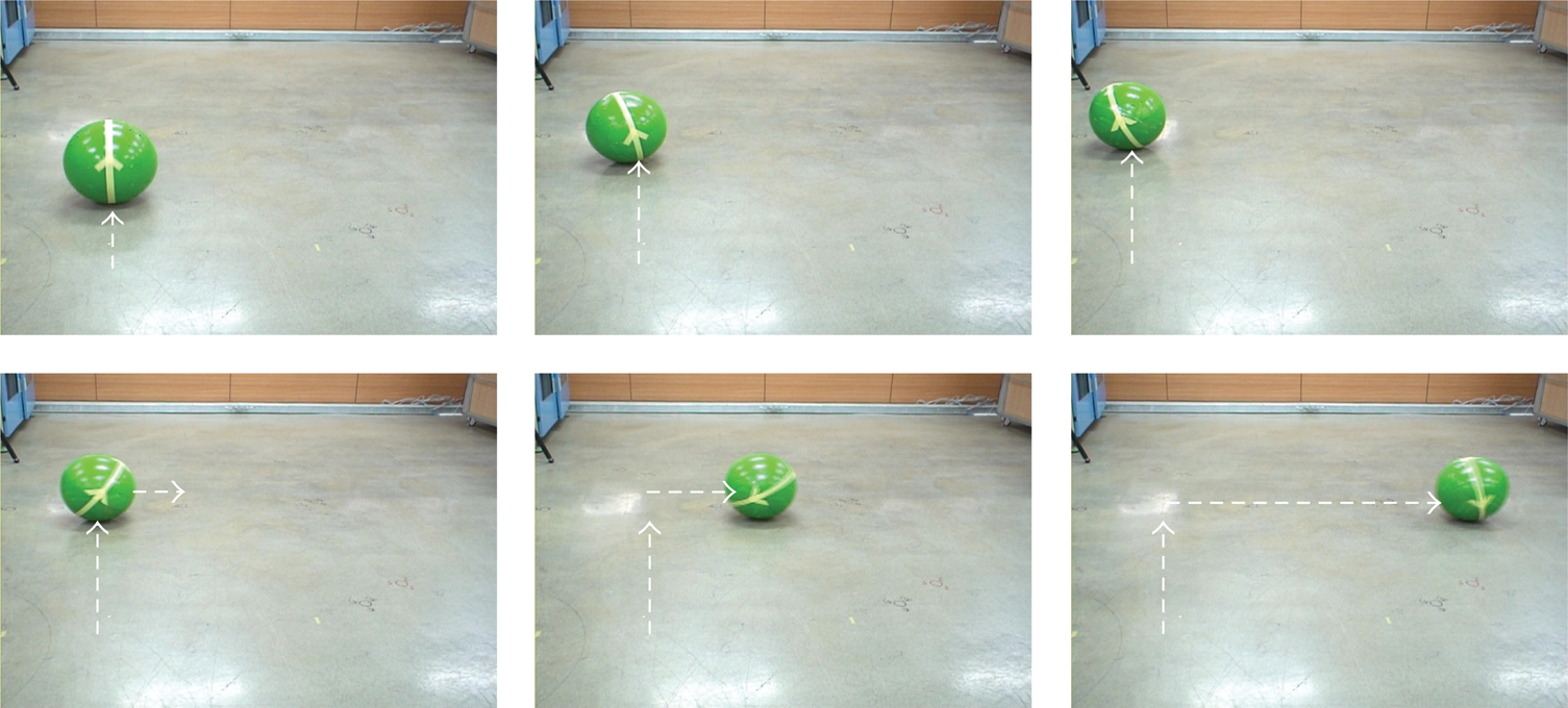
Snapshots of orthogonal driving.

The robot moves using base frame rotation and then stops for a short time to stabilize the pendulum. Thereafter, the robot moves using pendulum rotation in the previous driving direction orthogonally. In Figure 22, the top three pictures show the driving motion using base frame rotation, while the driving motion using pendulum rotation is shown in the bottom three pictures. As previously mentioned, the center rod of the base frame has a weight imbalance due to the position of the motors. This causes a deflected driving motion in the case of driving using base frame rotation, as shown in the top pictures of Figure 22. However, this problem can be resolved by a redesign of the mechanics, plus an appropriate attitude control algorithm would be also helpful.

Nonetheless, the experiment showed that KisBot II has the ability of orthogonal driving, which can be used for efficient obstacle avoidance, including a wall or valley. If the stopping ability and pendulum position control are improved, KisBot II could also perform high-speed orthogonal driving.

5. Conclusion

An upgraded version of a novel spherical robot with a hybrid two-pendulum driving mechanism, called KisBot II, was introduced to enhance the locomotion capability of conventional pendulum driven spherical robots. A linear motion equation using pendulum rotation was derived mathematically utilizing the Lagrange method. A nonlinear feedback controller was also constructed for linear driving using pendulum rotation based on a derived dynamic motion equation.

The upgraded KisBot II can achieve driving control and data communication using a task-based software architecture consisting of interrupt service routines. KisBot II can move in four directions from a stationary state, move in any direction using the base frame as a rudder when driving by pendulum, steer with a short turning radius, and travel orthogonally on the ground. Experiments also demonstrated that KisBot II has an improved locomotion capability when compared to conventional pendulum-driven spherical rolling robots.

However, we think that the unbalance weight of the internal mechanical structure could cause difficulties for controlling the driving velocity as one of the main reasons. Thus, the mechanical design of a spherical robot needs to take special consideration of the internal weight balance.

Future work will include the design of a simple structure for our robot. Plus, the driving difficulty due to uncertainties from the ground status and the mechanical structure of the outer shape should be solved through more research on the mathematical modeling for uncertainties and control methods, such as intelligent control including fuzzy control. Thus, with more functional improvements, KisBot II could be used for various applications and environments, including education, entertainment, security, military, and even planet exploration.

Conflict of Interests

The authors declare that there is no conflict of interests regarding the publication of this paper.

Footnotes

Acknowledgment

This research was supported by Kyungpook National University Research Fund, 2011.

References

Armour

R. H.

and Vincent

J. F. V.

, “Rolling in nature and robotics: a review,” Journal of Bionic Engineering, vol. 3, no. 4, pp. 195–208, 2006.

Halme

Schonberg

, and Wang

, “Motion control of a spherical mobile robot,” in Proceedings of the 4th International Workshop on Advanced Motion Control (AMC '96), pp. 259–264, Mie University, March 1996.

Bicchi

Balluchi

Prattichizzo

, and Gorelli

, “Introducing the “SPHERICLE”: an experimental testbed for research and teaching in nonholonomy,” in Proceedings of the IEEE International Conference on Robotics and Automation (ICRA '97), pp. 2620–2625, Albuquerque, NM, USA, April 1997.

lavadi

A. H.

and Mojabi

, “Introducing August: a novel strategy for an omnidirectional spherical rolling robot,” in Proceedings of the IEEE International Conference on Robotics and Automation, pp. 3527–3533, Washington, DC, USA, May 2002.

Bhattacharya

and Agrawal

S. K.

, “Design, experiments and motion planning of a spherical rolling robot,” in Proceedings of the IEEE International Conference on Robotics and Automation (ICRA '00), vol. 2, pp. 1207–1212, San Francisco, Calif, USA, April 2000.

Michaud

and Caron

, “Roball, the rolling robot,” Autonomous Robots, vol. 12, no. 2, pp. 211–222, 2002.

Kim

J. O.

Kwon

H. J.

, and Lee

J. H.

, “A rolling robot: design and implementation,” in Proceedings of the 7th Asian Control Conference, pp. 1474–1479, Hong Kong, August 2009.

Qiang

Tingzhi

Ming

, and Sanlong

, “Dynamic trajectory planning of a spherical mobile robot,” in Proceedings of the IEEE Conference on Robotics, Automation and Mechatronics, pp. 1–6, Bangkok, Thailand, June 2006.

Nagai

, Control system for spherical robot [M.S. thesis], Helsinki University of Technology, Espoo, Finland, 2008.

10.

Rotundus, http://www.rotundus.se.

11.

Kim

Y.-M.

Ahn

S.-S.

, and Lee

Y.-J.

, “KisBot: new spherical robot with arms,” in Proceedings of the 10th WSEAS International Conference on Robotics, Control and Manufacturing Technology (ROCOM '10), pp. 63–67, Hangzhou, China, April 2010.

12.

Zhao

, and Sun

, “Dynamics and motion control of a two pendulums driven spherical robot,” in Proceedings of the 23rd IEEE/RSJ 2010 International Conference on Intelligent Robots and Systems (IROS '10), pp. 147–153, Taipei, Taiwan, October 2010.

13.

Ghanbari

Mahboubi

, and Fakhrabadi

M. M. S.

, “Design, dynamic modeling and simulation of a spherical mobile robot with a novel motion mechanism,” in Proceedings of the IEEE/ASME International Conference on Mechatronic and Embedded Systems and Applications (MESA '10), pp. 434–439, Qingdao, China, July 2010.

14.

Joshi

V. A.

Banavar

R. N.

, and Hippalgaonkar

, “Design and analysis of a spherical mobile robot,” Mechanism and Machine Theory, vol. 45, no. 2, pp. 130–136, 2010.

15.

Sugiyama

Shiotsu

Yamanaka

, and Hirai

, “Circular/spherical robots for crawling and jumping,” in Proceedings of the IEEE International Conference on Robotics and Automation, pp. 3595–3600, Pisa, Italy, April 2005.

16.

T.-Y.

Zhang

X.-L.

Liu

Z.-Y

, and Zhang

Z.-N.

, “A tumbleweed-mimicing wind-driven rover for planetary exploration,” in Proceedings of the International Conference on Intelligent Computation Technology and Automation (ICICTA '10), pp. 42–45, May 2010.

17.

Yoon

J.-C.

Ahn

S.-S.

, and Lee

Y.-J.

, “Spherical robot with new type of two-pendulum driving mechanism,” in Proceedings of the 15th International Conference on Intelligent Engineering Systems (INES '11), pp. 275–279, Poprad, Slovakia, June 2011.

18.

Laplante

J.-F.

Masson

, and Michaud

, “Analytical longitudinal and lateral models of a spherical rolling robot,” Tech. Rep., Department of Electrical and Computer Engineering, Universite de Shebroke, Sherbrooke, Canada, 2007

Novel Spherical Robot with Hybrid Pendulum Driving Mechanism

Abstract

1. Introduction

2. Driving Mechanism and System Description of KisBot II

2.1. Design Concept

2.2. Motion Generation

2.3. Mechanical System Structure

2.3.1. Basic Structure and Motion Principles

2.3.2. Redesigned Outer Shell

2.4. Control System Structure

2.4.1. System Hardware

2.4.2. System Software

3. Motion Control for Linear Motion

3.1. Dynamic Model

3.2. Feedback Controller Design

4. Experimental Results

4.1. Linear Velocity Control in Pendulum Rotation Driving

4.2. Other Motion Generation

5. Conclusion

Conflict of Interests

Footnotes

Acknowledgment

References