The Bus Station Spacing Optimization Based on Game Theory

Abstract

With the development of city, the problem of traffic is becoming more and more serious. Developing public transportation has become the key to solving this problem in all countries. Based on the existing public transit network, how to improve the bus operation efficiency, and reduce the residents transit trip cost has become a simple and effective way to develop the public transportation. Bus stop spacing is an important factor affecting passengers’ travel time. How to set up bus stop spacing has become the key to reducing passengers’ travel time. According to comprehensive traffic survey, theoretical analysis, and summary of urban public transport characteristics, this paper analyzes the impact of bus stop spacing on passenger in-bus time cost and out-bus time cost and establishes in-bus time and out-bus time model. Finally, the paper gets the balance best station spacing by introducing the game theory.

1. Introduction

With the growing problem of urban traffic, the development of public transportation has become the key to solving the problem [1]. Based on existing public transportation network, how to improve the operational efficiency of the bus to reduce the cost of bus travel of residents has become a simple and effective way to develop public transportation [2]. Bus station spacing is an important factor affecting passenger travel time cost [3]. How to set up reasonable bus station spacing has become the key to reducing passengers’ travel time.

This study makes an analysis for the passenger leaving and waiting time at bus station, as well as the time cost for get on the bus and get off the bus. The summation of the three factors is the passenger out-bus time cost. The Thiessen polygon method is applied to divide the service areas of the stations. The space rectangular coordinate system is built up to derive the walking time cost. Furthermore, the effect of the bus station spacing on residents transit trip cost has been derived. The in-bus and out-bus time cost for the passengers are modeled. Finally, utilizing Nash two-person bargaining problems for the optimization of bus station spacing is an interesting measure.

2. Passenger Out-Bus Time Cost Research

2.1. Analysis of the Time Cost of Passenger to Leave Station

2.1.1. Bus Station Service Area Division

The total travel time of passengers depends on the service area of the bus station. The service radius of station is determined by walking distance and generally is about 500 m [4]. But for the division of the service area, previous studies generally used the circle method which simply assumes that the site is the center and the service radius is a circle redius. Although the method is simple and direct, the part of different service areas will overlap and some travel areas are not included in the service area that brings certain influence to the study of the passenger to leave station. In this paper, as an example of Nanjing 3 bus, based on service radius of 500 m, Thiessen polygon method is applied to divide the service areas of the stations [5]. Original site distribution and service area division are shown in Figure 1.

Figure 1:

Site distribution and service area division figure.

2.1.2. Walking Time Cost Calculation

Generally speaking, passengers by bus first are required to travel from the starting point to reach the bus lines and then walk along the bus route to the nearest bus station. Therefore, the distance for passengers to reach the bus station is divided into two parts: walking distance to the line and walking distance to the station [6].

(1) Walking Distance to the Line [7]. For a fixed bus route, the average distance of passengers walking to the line has little relations to do with the bus station spacing and through the establishment of space rectangular coordinate system is derived as shown in Figure 2. Coordinates of the cell centroid O _i is shown by (X _Oi , Y _Oi ). Coordinates of bus station S _i are shown by (X _Si , Y _Si ). The bus lines through the road R _j can be obtained by the coordinates of both ends. Its linear equation is A _j x + B _j y + C _j = 0. Draw a vertical line through cell centroid O _i to the bus lines through the road R _j to get straight line R _i : A _i x + B _i y + C _i = 0, pedal O _ri (X _Ori , Y _Ori ).

Figure 2:

Schematic figure of bus line plane rectangular coordinate system.

By plane analytic geometry can be obtained:

$\begin{array}{c}{X}_{Ori}=\frac{B_i^{\mathrm{2}}{X}_{Oi}-A_i{B}_i{Y}_{Oi}-A_i{C}_i}{A_i^{\mathrm{2}}+B_i^{\mathrm{2}}},\\ Y_{Ori}=\frac{A_i^{\mathrm{2}}{Y}_{Oi}-A_i{B}_i{X}_{Oi}-B_i{C}_i}{A_i^{\mathrm{2}}+B_i^{\mathrm{2}}}.\end{array}$

(1)

Therefore, distance to the line l₁ is the distance between centroid O _i and pedal O _ri that is obtained by calculating

$l_{\mathrm{1}}=\frac{\left|A_i{X}_{Oi}+B_i{Y}_{Oi}+C_i\right|}{\sqrt{A_i^{\mathrm{2}}+B_i^{\mathrm{2}}}}.$

(2)

(2) Walking Distance to the Station [8]. Based on the Tyson polygon method, the service area of each bus station is divided. So after drawing a vertical line from the starting point to the straight line that the bus travels, the location where pedal is has been identified in the service area of a station. The characteristic of passenger choosing site spacing cut-off point does not need to be analyzed and the choice of the upstream site or downstream site does not need to be considered. According to the above the Cartesian coordinates, walking distance to the station l₂ that the distance between pedal O _ri and site S _i can be obtained. Through solving, l₂ is obtained:

$l_{\mathrm{2}}=\left({\left(\frac{B_i^{\mathrm{2}}{X}_{Oi}-A_i{B}_i{Y}_{Oi}-A_i{C}_i}{A_i^{\mathrm{2}}+B_i^{\mathrm{2}}}-X_{Si}\right)}^{\mathrm{2}}\right)+{\left({\left(\frac{A_i^{\mathrm{2}}{Y}_{Oi}-A_i{B}_i{X}_{Oi}-B_i{C}_i}{A_i^{\mathrm{2}}+B_i^{\mathrm{2}}}-Y_{Si}\right)}^{\mathrm{2}}\right)}^{1/2}.$

(3)

To sum up, passenger walks distance to station L _w = l₁ + l₂. Its time cost T₁₁ is

$T_{\mathrm{11}}=\frac{L_w}{v_w}.$

(4)

v _w is passenger normal walking speed; its value is 5 km/h.

2.2. Analysis of the Time Cost of Site Waiting

Each passenger waiting time varies, but it is closely related to grid spacing and number of passengers arriving [9].

Let T₀ = 0 (T _l , l = 1, 2, …) indicate the time of Lth bus reaching bus station. Let J _l (l = 1, 2, …) indicate the intervals of two adjacent buses reaching bus stations, J _l = T _l − T_{l − 1}. Let F(t) be the distribution function of J _i . The mean of F(t) = P (J _l ≤ t), l = 1, 2, …, is μ₁. The variance of F(t) is d.

Assume that passengers arrive at the bus station with Poisson stream of intensity λ₁ and that the number of passengers who arrive at the bus station is N(t) at any time (0, t). Based on the nature of Poisson, P[N(t) = k] = ((λ₁t) ^k /k!)e − λ₁ ^t is obtained. s(J _l ) indicates arriving passengers who are waiting for the bus at cumulative waiting time in the time [T_{l − 1}, T _l ]. N(J _i ) indicates the number of passengers who are waiting for the bus in the time [T_{l − 1}, T_{l − 1} + J _l ].

In the time [T_{l − 1}, T _l ], the waiting time of the first k passengers is (J _l − s _k ). In the time [T_{l − 1}, T _l ], the cumulative waiting time of passengers is

$s\left(J_l\right)=\left(J_l-s_{\mathrm{1}}\right)+\left(J_l-s_{\mathrm{2}}\right)+\cdots +\left(J_l-s_{N\left(J_l\right)}\right)={{\displaystyle \sum }}_{k=\mathrm{1}}^{N\left(J_l\right)}\left(J_l-s_k\right).$

(5)

Based on the nature of the Poisson stream,

$E\left[s\left(J_l\right)\mid N\left(J_l\right)=r\right]=E\left[{{\displaystyle \sum }}_{k=\mathrm{1}}^{N\left(J_l\right)}\left(J_l-s_k\right)\mid N\left(J_l\right)=r\right]=E\left[{{\displaystyle \sum }}_{k=\mathrm{1}}^r\left(J_l-s_k\right)\mid N\left(J_l\right)=r\right]=r{J}_l-E\left[{{\displaystyle \sum }}_{k=\mathrm{1}}^r{s}_k\mid N\left(J_l\right)=r\right]=r{J}_l-{{\displaystyle \sum }}_{k=\mathrm{1}}^{r}E\left(U_k\right)=\frac{r{J}_l}{\mathrm{2}}.$

(6)

Based on conditions desired properties, in the time [T_{l − 1}, T _l ], the cumulative average waiting time of passengers is

$E\left[s\left(J_l\right)\right]={\displaystyle \sum }_{r=\mathrm{0}}^{\infty }E\left[s\left(J_l\right)\mid N\left(J_l\right)=r\right]·P\left[N\left(J_l\right)\right]=r=\frac{{\lambda }_{\mathrm{1}}{J}_l^{\mathrm{2}}}{\mathrm{2}}.$

(7)

Thus, the cumulative average waiting time of passengers in the time interval of any two adjacent buses leaving the bus station is deduced:

$E\left(s\right)={{\displaystyle \int }}_{\mathrm{0}}^{\infty }\frac{{\lambda }_{\mathrm{1}}}{\mathrm{2}}{t}^{\mathrm{2}}dF\left(t\right)=\frac{{\lambda }_{\mathrm{1}}}{\mathrm{2}}{{\displaystyle \int }}_{\mathrm{0}}^{\infty }{t}^{\mathrm{2}}dF\left(t\right)=\frac{{\lambda }_{\mathrm{1}}}{\mathrm{2}}E\left(J_l^{\mathrm{2}}\right)=\frac{{\lambda }_{\mathrm{1}}}{\mathrm{2}}\left[E^{\mathrm{2}}\left(J_l\right)+D\left(J_l\right)\right]=\frac{{\lambda }_{\mathrm{1}}}{\mathrm{2}}\left({\mu }_{\mathrm{1}}^2+d\right).$

(8)

From the above equation, the two factors, bus arrival time interval and passengers arrival strength, affect cumulative waiting time of passengers.

Per capita average waiting time is

$T_{\mathrm{12}}=\frac{\mathrm{1}}{\mathrm{2}}\left({\mu }_{\mathrm{1}}^2+d\right).$

(9)

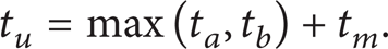
2.3. Site Passengers up and down Time Cost Analysis

In this section, the studies of passengers up and down time cost is that time cost of a passenger up and down as research subjects includes the time of a passenger up and down at the bus station and the time of door switching in the travel process [10]:

$T_{\mathrm{13}}=t_{uO}+t_{uD}=\max \left(t_{aO},t_{bO}\right)+\max \left(t_{aD},t_{bD}\right)+\mathrm{2}{t}_m.$

(10)

t _uO , t _uD are the time of a passenger up and down at the bus starting and finishing site.

In summary, the out-bus time of unit passenger is

$T_{\mathrm{1}}=T_{\mathrm{11}}+T_{\mathrm{12}}+T_{\mathrm{13}}.$

(11)

3. Passenger In-Bus Time Cost Research

3.1. Bus Normal Travel Time Cost Analysis

On the road of no stops and intersection assuming that bus travels without the effect of other vehicles, the bus travels with constant speed v _b . So the traveling time of the bus is stationary. Its expression is

$t_r=\frac{L_c}{v_b}.$

(12)

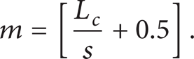
• t _r is the normal traveling time of the bus.

• L _c is the average distance for each passenger taking the bus.

• v _b is the average traveling speed of the bus on the road.

3.2. Bus Delay Time Cost Analysis

3.2.1. Bus Delay in the Intersection

The delay time of the bus in the intersection is affected by signal cycle, signal green ratio, queuing vehicle length of the intersection, vehicle flow at intersection, and the time of the bus arriving at the intersection. In addition, bus delay in the intersection is related to bus lane. Therefore, the delay time of the bus in the intersection is affected by many factors [11].

Assuming that in the time T the average saturation of an import road in the intersection is x _i , signal cycle length is always C, the red light length is r, the green light length is g, and the number q of vehicles arriving at the intersection in the signal cycle obeys Poisson distribution, recorded as q ∼ π(λ₂). The saturation value of the vehicle reaching the intersection in the signal cycle is q _c . The headway of two adjacent vehicles in the queuing traffic is t₀. The saturated queue length in the cycle is L₀. If q > L₀, traffic appears supersaturated and there is the vehicle secondary parking. Assume that the time of vehicle reaching the intersection obeys uniform distribution. So the time interval of two adjacent buses is c/(q + 1).

Calculate the delay time of the vehicle in the intersection with each signal cycle.

If q ≤ L₀, the total traffic delays time is

$D_q={{\displaystyle \sum }}_{i=\mathrm{1}}^q\max \left[r-\frac{ic}{q+\mathrm{1}}+\left(i-\mathrm{1}\right)t_{\mathrm{0}},\mathrm{0}\right].$

(13)

If q > L₀, the total traffic delays time is

$D_q={{\displaystyle \sum }}_{i=\mathrm{1}}^q\left[r-\frac{ic}{q+\mathrm{1}}+\left(i-\mathrm{1}\right)t_{\mathrm{0}}\right]+\left(q-L_{\mathrm{0}}\right)r.$

(14)

Q is 1, 2, …. The probability of q _c is p₁, p₂, …, p _qc . If the average saturation is x _i , the total delay of vehicles on import road of the intersection with each cycle is

$D_c={{\displaystyle \sum }}_{i=\mathrm{1}}^{q_c}{p}_i{D}_i.$

(15)

The average delay of all vehicles, namely the bus delay at intersection is:

$d_c=\frac{D_c}{{\lambda }_{\mathrm{2}}}.$

(16)

3.2.2. Bus Delay in the Station

Bus delay in the station is the difference between the time from bus driving into bus stations to exiting the bus stations and the time that bus leaves the site, mainly including deceleration delay, queuing delay, and leaving acceleration delay. The delay is mainly related to the bus models and performance, the size of the platform, platform arrangement, the number of bus stop lines of each site, and the number of waiting passengers [12].

Based on the investigation of inbound and departure time of Nanjing 3 bus different sites, the distribution of deceleration time when the bus travels into the station and the distribution of acceleration time when the bus leaves the station are concluded, respectively, as shown in Figures 3 and 4.

Figure 3:

Vehicles stop the distribution of deceleration time figure in the bus station.

Figure 4:

Vehicles outbound the distribution of acceleration time figure in the bus station.

The figure shows that the buses stop deceleration and outbound acceleration time delay has no certain regularity, so it is needed to take the average of two kinds of delays. That is,

$da=\mathrm{6.88}+\mathrm{11.03}=\mathrm{17.9}.$

(17)

Multiple line bus stops, especially the bus station of the main road or the central region of many large and medium cites, usually have more than one location, some large bus stations even have three or four parking positions. The buses lining up for stop is a simple type of queue, and first in first out. So the site can be seen as M/M/N system of single line and multichannel service. Through calculating the corresponding index of the system, the average delay time of bus lining up in the station can be concluded. The specific calculation process is as follows.

Set in the bus station that vehicle arrival law obeys Poisson distribution of parameter λ₃, the vehicle carrying capacity of bus station obeys negative exponential distribution of parameter μ₃, and the number of the parking positions of the station is n₀.

The service intensity of the bus station is

$\rho =\frac{{\lambda }_{\mathrm{3}}}{n_{\mathrm{0}}{\mu }_{\mathrm{3}}}.$

(18)

The probability of no buses parking in the station is

$P\left(\mathrm{0}\right)=\frac{\mathrm{1}}{{\sum }_{k=\mathrm{0}}^{n-\mathrm{1}}\left({\rho }^k/k!\right)+\left({\rho }^n/n_{\mathrm{0}}!\left(\mathrm{1}-\rho /n_{\mathrm{0}}\right)\right)}.$

(19)

The average queue length of the station is

$\overline{q}=\frac{{\rho }^{n+\mathrm{1}}}{n_{\mathrm{0}}!n_{\mathrm{0}}}·\frac{P\left(\mathrm{0}\right)}{{\left(\mathrm{1}-\rho /n_{\mathrm{0}}\right)}^{\mathrm{2}}}.$

(20)

The average queuing delay is

$d_w=\frac{\overline{q}}{{\lambda }_{\mathrm{3}}}.$

(21)

3.3. The Bus Stopping Time Cost Analysis

Based on the above analysis, the bus stops time at the site including the bus at the site of the opening hours, passengers up and down time, and closing time. Because the switch gate time is a fixture, which is generally 1∼3 s, the proportion is very small, so the buses’ stopping time depends largely on the upper and lower time. The get-on (or get-off) time is propositional to the product of the passenger get-on (or get-off) volume and the average of the get-on (or get-off) time for all passengers, where the average time is in terms of the vehicle's structure, the payment measure, the passenger's characteristic, the crowded level and the disturbance to the passengers [13]. According to the investigations, the relationships of boarding/getting off time and boarding/getting off volume are given in Figures 5 and 6, respectively.

Figure 5:

Relation between boarding time and boarding passenger volume at bus stops.

Figure 6:

Relation between getting off time and getting off passenger volume at bus stops.

From the linear regression fitting on the investigation data, the relationships between bus service times and passenger volumes are given as follows:

$\begin{array}{c}{t}_a=\mathrm{1.990}{n}_a+\mathrm{2.029},\\ t_b=\mathrm{1.039}{n}_b+\mathrm{2.133}.\end{array}$

(22)

n _a , n _b are get on the bus and get off traffic, respectively.

In conclusion, the bus stop time is

$t_u=\max \left(t_a,t_b\right)+t_m.$

(23)

3.4. Passenger In-Bus Time Cost Model

Through the above analysis, the normal driving time, delay, and stop time for buses are obtained. To find out the reasonable bus station spacing, this study focuses on the passenger in-car time [14].

Like (1), L _c is the average distance of the passenger taking the bus. Hypothesis L is average bus station spacing, unit of passenger travel starting site is S _i , and purpose of the site is S_{i + n}; there are

$n=\left[\frac{L_c}{L}+\mathrm{0.5}\right].$

(24)

Assume that the road that the bus travels on average every s (m) has an intersection. The unit passenger bus number is required to pass through intersection

$m=\left[\frac{L_c}{s}+\mathrm{0.5}\right].$

(25)

Passengers in the first S _i and S_{i + n} stand, respectively, accelerate away from the station and deceleration process station. In the first S_{i + 1} ∼ S_{i + n − 1} station is slow pit stop, accelerating away from the station. So the unit in the process of the bus passengers has a total of n deceleration delays. At the same time also it experienced a process of bus line stops n times.

For stopping time, except the boarding time and getting off time, passengers experienced n − 1 times bus station stopping.

In conclusion, in-car time of one passenger is

$T_{\mathrm{2}}=t_r+\left(m·d_c+n·d_a+n·d_w\right)+\left(n-\mathrm{1}\right)t_u.$

(26)

4. Station Spacing Optimization Based on Game Theory

4.1. Nash Bargaining Solution

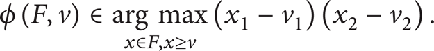
For bargaining problems (F, v), its purpose is to find a reasonable configuration from F ∩ {(x₁, x₂)∣x₁ ≥ v₁, x₂ ≥ v₂} and get the resulting configuration notes for φ(F, v), which is bargaining solution function of the problem.

Nash bargaining solution has the following five axioms [15]:

1. individual rationality,

2. strong Pareto efficiency,

3. symmetry,

4. the invariance of the equivalent profit description,

5. the independence of the independent choice.

In the case of meeting the five axioms, Nash proved that the two-person bargaining problem has only a bargaining solution.

Bargaining for two people (F, v), which meet the only bargaining solution of axiom 1–5, the solution (x₁, x₂) maximizes the Nash product (x₁ − v₁)(x₂ − v₂). Or its bargaining solution is the solution of the following question:

$\varphi \left(F,v\right)\in \underset{x\in F,x\ge v}{\arg \hspace{0.17em}\max }\left(x_{\mathrm{1}}-v_{\mathrm{1}}\right)\left(x_{\mathrm{2}}-v_{\mathrm{2}}\right).$

(27)

4.2. Spacing Optimization Based on Nash Bargaining Two Sites

4.2.1. Basic Assumptions

According to the account of previous chapters, we can see that total passenger bus travel time can be divided into outside and inside the car time, while the site space affects the two times. Regarding the out side bus and inside bus costs as two rational players. It is that the reduction of the outside cost will inevitably increase the inside cost, and reducing the inside costs will increase the cost of outside car. In order to make the two combined, that is, to minimize the cost, passenger bus travel will introduce two-person Nash bargaining problems. So define the following parameters [16]:

• L _min : site spacing can reach the minimum,

• L _max : site spacing can reach the maximum,

• L_*: the optimal value of site spacing,

• T_{1min ⁡}: the outside car cost minimum,

• T_1max: the outside car cost maximum,

• T_1*: the outside car cost optimal value,

• T_2min: the inside car cost minimum,

• T_2max: the inside car cost maximum,

• T_2*: the inside car cost optimal value.

Assuming that the outside car cost T₁ and the inside car cost T₂ to cooperation and competition, there are two strategies, respectively: the individual optimal and consider the overall optimal inward. Have the game model shown in Table 1.

Table 1:

The outside car and the inside car costs game model.

	The outside car cost T1
	Individual optimal	Overall optimal
The inside car cost T2
Individual optimal	—	(T1 max ⁡, T2 min ⁡)
Overall optimal	(T1 min ⁡, T2 max ⁡)	(T1*, T2*)

Obviously, the T₁ and T₂ at the same time to be the optimum are not possible. When the T₁ consider overall optimal and T₂ is still on the premise of its own optimal, T₁ in order to accommodate the T₂ is bound to get maximum value; with be T₂ to consider the overall optimal and T₁ is still on the premise of its own optimal, T₂ shall take maximum. Three of the passengers in the total time of transit mode are not optimal. Only when the T₁ and T₂ considering overall optimal at the same time, to get the minimum total time cost.

4.2.2. The Optimal Station Spacing Solving

Through the above assumption and analysis, there can be a game between the outside car and the inside car costs as two-person bargaining problems. In order to maximize the overall interests of T₁ and T₂, the bargaining problems are needed to be solved to conclude the optimal solution, T₁* and T₂*.

The problem is different from general bargaining problems, the desire of the optimal solution is the minimum value of T₁ + T₂, and so Nash product for the problem is (T_{1max ⁡} − T₁)(T_{2max ⁡} − T₂). It is to solve the problem

$\max \left(T_{\mathrm{1}\max }-T_{\mathrm{1}}\right)\left(T_{\mathrm{2}\max }-T_{\mathrm{2}}\right).$

(28)

(1) Solving T_1max. When the largest site spacing is achieved, the maximum of passenger outside car costs is found. Assume that there are only the first and last stations, the time costs for walking outside car will increase. Set the original bus lines at the end of the first and station, respectively, are S₀ and S _N . Passengers travelling during site S _i , site distribution and passengers point diagram shown in Figure 7.

Figure 7:

The spacing between the original site of the site distribution diagram and the passengers.

When the site is from N + 1 to 2 for now, walking distance to the station for the passengers is

$l_{\mathrm{2}}^{\prime }=iL-{\left(-\mathrm{1}\right)}^{\tau }{l}_{\mathrm{2}}.$

(29)

τ: change the site before the number of passengers takes 1 upstream site selection, when choosing downstream site take 0. The below is the same.

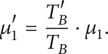
Due to the decrease in the number of sites, the bus running time will also be reduced; the bus service frequency changes. Assume that the bus departure time interval is proportional to the bus running time. Can by solving site quantity change before and after the bus running time, get the new departure time interval, having been further new passenger waiting time:

$\begin{array}{c}{T}_B=t_r+\frac{L_B}{s}{d}_c+N\left(d_a+d_w+t_u\right),\\ T_B^{\prime }=t_r+\frac{L_B}{s}{d}_c+\mathrm{2}\left(d_a+d_w+t_u\right).\end{array}$

(30)

• T _B , T _B ′ are, respectively, to reduce site bus before and after running all the time.

• L _B is that the bus runs all the distance.

The departure interval time averages can be obtained after reducing the site:

${\mu }_{\mathrm{1}}^{\prime }=\frac{T_B^{\prime }}{T_B}·{\mu }_{\mathrm{1}}.$

(31)

In conclusion, the maximum available passengers outside the car cost are

$T_{\mathrm{1}\max }=T_{\mathrm{11}}^{\prime }+T_{\mathrm{12}}^{\prime }+T_{\mathrm{13}}=\frac{l_{\mathrm{1}}+l_{\mathrm{2}}^{\prime }}{v_w}+\frac{{\lambda }_{\mathrm{1}}^{}}{\mathrm{2}}\left({\mu }_{\mathrm{1}}^{\prime \mathrm{2}}+d\right)+T_{\mathrm{13}}.$

(32)

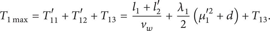
(2) Solving T_2max. When site spacing is very small, passenger car costs would be great. It increases the dock delays and the stop time. Dividing the original site spacing into l₂ parts, which means that the distance to the site from the travel point includes the walking distance only, passengers reaching the bus line indicates they reach the site. The beginning and the end of the passenger bus sites are, respectively, S _i ′ and $S_{i+n·l_{\mathrm{2}}-\mathrm{1}}^{\prime }$ (the original to the upstream station S _i ) or S _i ′ and $S_{i+n·l_{\mathrm{2}}+\mathrm{1}}^{\prime }$ (the original to the downstream station), as shown in Figure 8.

Figure 8:

Equal to the original site spacing after passengers aboard a site map.

At this time for passenger, car cost is

$T_{\mathrm{2}\max }=t_r+m·d_c+\left(n·l_{\mathrm{2}}+\mathrm{1}-\mathrm{2}\tau \right)\left(d_a+d_w\right)+\left(n·l_{\mathrm{2}}-\mathrm{2}\tau \right)t_u.$

(33)

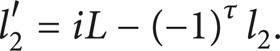
(3) Nash Product Solution. In conclusion, we can get Nash product expression:

$\left(T_{\mathrm{1}\max }-T_{\mathrm{1}}\right)\left(T_{\mathrm{2}\max }-T_{\mathrm{2}}\right)\hspace{0.5em}=\left[\frac{l_{\mathrm{2}}^{\prime }-l_{\mathrm{2}}}{v_w}+\frac{\mathrm{1}}{\mathrm{2}}\left({\mu }_{\mathrm{1}}^{\prime \mathrm{2}}-{\mu }_{\mathrm{1}}^2\right)\right]\left[\left(l_{\mathrm{2}}-\mathrm{1}\right)n+\mathrm{1}-\mathrm{2}\tau \right]·\left(d_a+d_w+t_u\right),$

(34)

where l₂′ = iL − (− 1)^τl₂, n = [L _c /L + 0.5] is the function for L, and the rest of the parameters are constants that can be measured, so to simplify the above formula,

$\left(T_{\mathrm{1}\max }-T_{\mathrm{1}}\right)\left(T_{\mathrm{2}\max }-T_{\mathrm{2}}\right)=\left(A_{\mathrm{1}}L+B_{\mathrm{1}}\right)\left(\frac{A_{\mathrm{2}}}{L}+B_{\mathrm{2}}\right).$

(35)

Put L in (35) derivative, and make it equal to zero; getting the Nash bargaining solution is the bus station spacing of the optimal solution:

$L^{*}=\sqrt{\frac{A_{\mathrm{2}}{B}_{\mathrm{1}}}{A_{\mathrm{1}}{B}_{\mathrm{2}}}}.$

(36)

5. Summary

In this paper, the author made the division of all the bus stops service area by the Thiessen polygon method to build plane rectangular coordinate system and bring the passenger travel time model as the result. Compared with the method of building plane rectangular coordinate system directly, it is clear that which site can be used for the passengers travelling at different points. This paper omits the step that computes in which site passengers get on the bus. In the study of the bus stopping time, the author introduced the single multichannel queuing service system which is widely used in traffic engineering to study the bus stops queuing time. The model of the relation between the car time and site space was built based on the comprehensive analysis of passengers’ time at every stage in the car. Finally the author introduced the game theory of Nash two-person bargaining problems and assumes that the two sides are the vehicle external time and the vehicle interior time. On the basis of Nash bargaining solution, the paper gets the bus-site spacing when vehicle external time and the vehicle interior time sum is minimal.

The limitation of this study is that the influence of the traffic flow at peak hours has not been taken into consideration. This effect should be involved in the future study.

Conflict of Interests

The authors declare that there is no conflict of interests regarding the publication of this paper.