Solving Minimum Cost Three-Dimensional Localization Problem in Ocean Sensor Networks

Abstract

Localization is one of the most fundamental problems in wireless sensor networks (including ocean sensor networks). Current localization algorithms mainly focus on how to localize as many sensors as possible given a set of mobile or static anchor nodes and distance measurements. In this paper, we consider an optimization problem, the minimum cost three-dimensional (3D) localization problem, in an ocean sensor network, which aims to localize all underwater sensors using the minimum number of anchor nodes or the minimum travel distance of the surface vessel which deploys and measures the anchors. Given the hardness of 3D localization, we propose a set of greedy methods to pick the anchor set and its visiting sequence. Aiming at minimizing the localization errors, we also adopt a confidence-based approach for all proposed methods to deal with noisy ranging measurements (which is very common in ocean sensor networks) and possible flip ambiguity. Our simulation results demonstrate the efficiency of all proposed methods.

1. Introduction

Localization is one of the most challenging tasks in designing ocean sensor networks [1–3] or general wireless sensor networks [4–6], which aims to obtain the physical locations of each individual sensor node. Location information can be used in many tasks of ocean sensor networks such as event detecting, target/device tracking and coverage, environmental monitoring, tagging raw sensing data, and network deployment. In most of these ocean sensing applications, acquiring localization information is an essential part of the sensing tasks. For example, ocean survey data acquired by sensors are useless without correct location information; target tracking needs the accuracy of location information and distance measurement. Moreover, location information can also be used by certain networking protocols to enhance the performance of ocean sensor networks, such as routing packets using position-based routing [7, 8] or controlling the network topology and coverage using geometric methods [7, 9].

It is more challenging to locate nodes in underwater environments than in terrestrial environments. First, GPS signal does not propagate through water and RF signal cannot be used since it will attenuate very rapidly in water. Thus, acoustic signal is usually the best choice in underwater environments. Second, several alternative cooperative positioning schemes are not applicable in practice due to acoustic channel properties (such as low bandwidth, high propagation delay, and high bit error rate). Since the velocity of acoustic signal can change with salinity, pressure, and temperature, it is difficult to get quite precise ranges between nodes underwater. Last, the three-dimensional (3D) deployment of ocean sensor network requires more anchor nodes to locate nodes in 3D ocean space. All these make accurate 3D localization in ocean an extremely challenging task.

In recent years, a large number of localization techniques [10–17] have been proposed for ocean senor networks to localize underwater sensors by exchanging information with anchor nodes. However, most of them try to localize sensors without the guarantee of covering all sensors. They usually rely on one hypothesis that there are enough anchor nodes to achieve the goal. Recently, Huang et al. [18] introduce a new localization problem, called minimum cost localization problem (MCLP), for 2D sensor networks which aims to localize all nodes in a network using minimum anchor nodes. In this paper, we extend the optimization problem to 3D ocean sensor networks to form a minimum cost 3D localization problem (MC3DLP). Note that the cost of manually configuring an anchor node in ocean is expensive and GPS device does not work well underwater. Therefore, we rely on a sea surface vessel visit to deploy and find the locations of anchor nodes. Thus, we also include a new variation of MC3DLP where the length of visited path for the vessel is considered as the optimization objective. For both versions of MC3DLP, we propose multiple greedy algorithms to localize all underwater sensors with the minimum number of anchors or the minimum travel distance of the surface vessel. Note that both MCLP and MC3DLP focus on minimizing the localization cost and assume that the localization phase is accurate, which may not be true in reality.

In addition, to handle localization errors caused by both ranging errors and flip ambiguity, we introduce a confidence-based approach to control errors induced in localization process. This is critical for 3D ocean sensor networks, since acoustic propagation in ocean varies with different salinity, pressure, and temperature, which may lead to larger ranging errors during the localization phase. Our simulation results over random 3D ocean sensor networks demonstrate the efficiency and effectiveness of all proposed methods.

The rest of this paper is organized as follows. We first briefly review related work on 2D/3D localization techniques in Section 2. We introduce our models and assumptions about ocean networks in Section 3. The minimum cost 3D localization problems are then formally defined in Section 4. A set of greedy algorithms are designed and presented in Section 5 aiming at solving the MC3DLP. Section 6 discusses how to handle the localization errors which are very common in ocean sensor networks. Section 7 presents our simulation results over random ocean sensor networks. Finally, Section 8 concludes this paper. A preliminary conference version of this paper appeared in [19].

2. Related Work

To fulfill different requirements of localization tasks in ocean sensor networks, various 3D localization methods have been proposed [10–17]. Most of these methods can be classified into two categories: range-based methods and range-free methods. Range-based methods utilize time of arrival (ToA) [10–12] or time difference of arrival (TDoA) [13–15] to measure distances between nodes and then use these distance estimations to compute positions of nodes. Usually, in range-based methods, a certain number of anchor nodes are used, whose positions are known beforehand or can be measured by sea surface buoys or vessels. Range-free methods [16, 17] do not employ accurate measurement techniques; instead, they use alternative methods such as hop count or areas to locate nodes with lower cost. However, they usually provide coarse accuracy. In this paper, we consider range-based localization methods where acoustic signals are used for estimating the distance between underwater sensors. Some comprehensive surveys on localization in ocean sensor networks can be found in [1–3].

The minimum cost localization problem (MCLP) is first introduced for 2D wireless sensor networks by [18]. Given the set of sensors and distance measurements among them, it aims to find an anchor set such that (1) the whole network could be localized and (2) the total cost of setting up these anchors is minimized. This is a completely different problem from previous works on localization. The authors show that such a problem is very challenging and then present a set of greedy algorithms using both trilateration and local sweep operations to address the problem. Recently, a genetic algorithm for the MCLP is also proposed by [20]. All these studies tackle MCLP in 2D cases where at least three distance measurements are needed to localize a sensor node. In this paper, we further extend and enhance the problem within 3D ocean sensor networks by considering 3D deployment, course of the surface vessel, and possible noise measurements, which are all unique for 3D ocean sensor networks compared with 2D terrestrial sensor networks.

3. Models and Assumptions

The 3D ocean sensor network can be modelled as a graph $G=(V,E)$ , in which V is the set of nodes representing underwater sensor nodes and E is the set of links connecting sensor nodes if they are within each other's sensing range. Here, we assume all sensor nodes are static, ignoring the movement caused by subsurface current. We also assume that the sensing range r of all sensor nodes is the same; however, our model and solutions can be easily modified to deal with a more general case where sensor nodes may have different sensing ranges. In addition, we assume that communication ranges of sensors are larger than their sensing ranges so that all estimated distances among E could be collected via multihop communications. A subset of sensor nodes $B\subset V$ will be defined as anchor nodes whose positions need to be known at the beginning of localization (i.e., deployed and measured by a sea surface vessel visit). Note that GPS devices do not work underwater. The remaining widely distributed underwater sensor nodes will rely on distance measurements in E and the positions of anchor nodes B to determine their locations during the localization procedure. Underwater sensor nodes maybe distributed in different depths, but only those shallow sensor nodes can be captured by a surface vessel's sensing range. Thus, we assume that only the shallow sensors can be considered to become anchor nodes. We use $V^{\prime }\subset V$ to denote the set of shallow sensor nodes. We also assume that the surface vessel can accurately localize all selected anchors, which are either on or near the sea surface, given the vessel is usually equipped with more powerful localization devices. The location of surface vessel can be obtained by GPS. The GPS signal in space can provide a “worst case” pseudorange accuracy of 7.8 meters at a 95% confidence level [21]. Combined with augmentation systems, the accuracy of real-time positioning can increase to centimeter level. See Figure 1 for illustration. Note that it is possible that some underwater sensor nodes cannot be localized even though all shallow sensor nodes become anchors. Therefore, we assume that V only contains sensor nodes which are localizable when all shallow sensor nodes are set as anchors. We summarize all symbols used in this paper (see Symbols section).

Figure 1

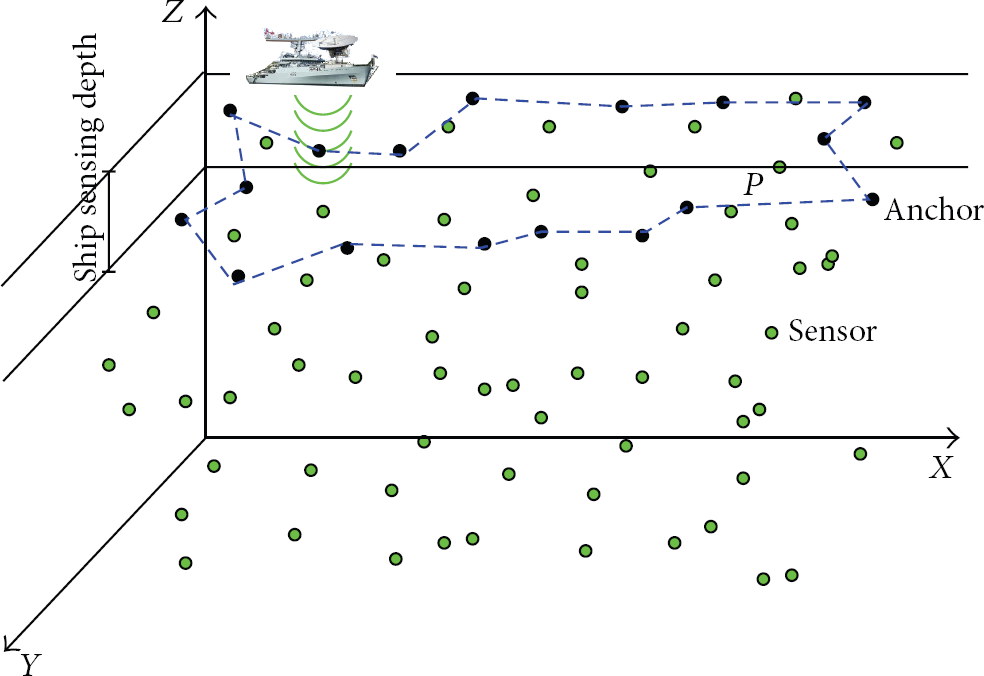
Illustration of localization scenario in 3D ocean sensor networks. Black nodes are selected anchors from the shallow sensor nodes, while other green nodes are localized via localization method. P represents the traveling path of the sea surface vessel to visit all anchors.

4. Minimum Cost 3D Localization Problem

The main purpose of the minimum cost 3D localization problems (MC3DLPs) in a 3D ocean sensor network is to localize all underwater nodes in the network using the minimum cost for anchor nodes. The cost includes the equipment cost and any costs during deployment and measurement.

Similar to [18], by assuming a unit cost per anchor node, we can define the following MC3DLP problem.

Definition 1 (minimum cost 3D localization problem 1 (MC3DLP-1)).

Given a 3D ocean sensor network G, find a subset B of shallow sensor nodes to be anchor nodes such that (1) all sensor nodes in V can be localized given the graph, the length of all links, and positions of all anchor nodes and (2) the total number of anchor nodes $\left|B\right|$ is minimized.

In addition to the cost per anchor node, the cost of deployment and measurement for all anchors may depend on the length of the route P travelled by the sea surface vessel (shown in Figure 1). In that case, the MC3DLP problem can be defined as follows.

Definition 2 (minimum cost 3D localization problem 2 (MC3DLP-2)).

Given a 3D ocean sensor network G, find a subset B of shallow sensor nodes to be anchor nodes such that (1) all sensor nodes in V can be localized given the graph, the lengths of all links, and positions of all anchor nodes and (2) the total length of the route $\parallel P\parallel$ taken by the sea surface vessel to visit all anchors is minimized.

It is clear that both MC3DLPs always have a feasible solution, since based on our assumption in the worst case all shallow sensors are selected as anchors (i.e., $B=V^{\prime }$ ) and all sensors in V will be localized. However, finding the optimal solution of such problems is still very challenging. Since the 2D MCLP [18] is a special case of MC3DLP-1 and it is NP-hard, MC3DLP-1 is also NP-hard. In MC3DLP-2, without considering the localization part, finding the minimum length route to visit all anchors alone is the well-known travel salesman problem (TSP), which is NP-hard. Therefore, MC3DLP-2 is also at least NP-hard.

5. Minimum Cost 3D Localization Algorithms

In this section, we introduce different greedy algorithms to approximately solve MC3DLP problems by finding the anchor set. All proposed greedy algorithms use a simple color coding, where each sensor node v will be marked with different colors to represent its current status. We use $s(v)$ to denote v's color and status. A white sensor node represents the node which has not been localized yet; a black sensor node denotes the selected anchor node which can be directly contacted by the surface vessel to get its position; a green sensor node is a nonanchor node whose location can be obtained via localization. Initially, all sensor nodes are white. The purpose of our algorithms is to find the smallest set of anchors (black nodes) or the anchor set with the minimum traveling distance to get the positions of all nodes (coloring all nodes in either black or green) as shown in Figure 1.

5.1. Algorithms for MC3DLP-1

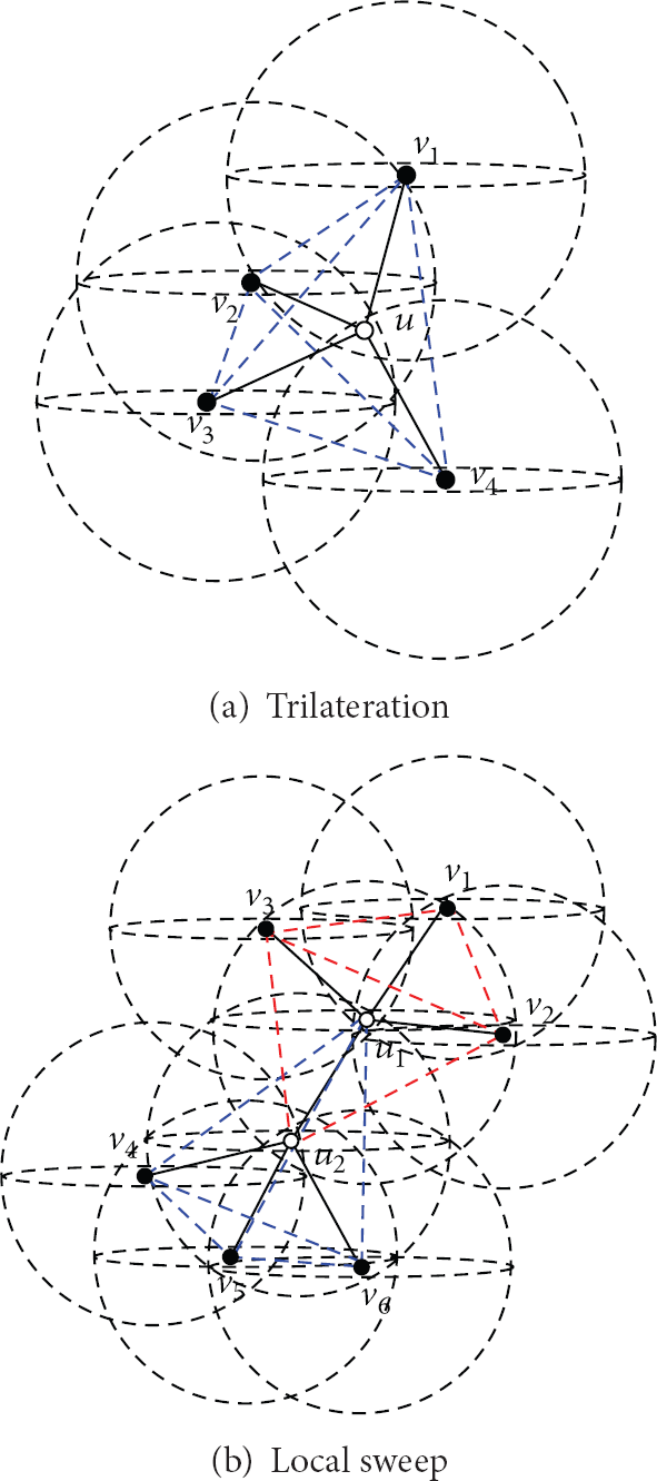
For solving the MC3DLP-1, we simply extend two proposed methods in [18] for 2D MCLP (one uses trilateration and the other uses local sweep for localization) to 3D networks. Both methods use a general greedy framework as shown in Algorithm 1. The basic idea is as follows. Initially, all sensor nodes will be colored white and with its rank $r(v)=0$ (Lines 1-2). Here, node rank $r(v)$ of a node v indicates the total count of localized neighbors (with color of black or green). In addition, any sensor nodes with less than four neighbors will be marked as black (Lines 3–5), since they cannot be localized by others. Note that, based on our assumption, all these nodes are shallow sensor nodes. Then, in each step (Lines 6–13) the algorithm greedily picks one white sensor node which can benefit the localization procedure most in the next step if it is marked as black and colors it black. Here, we define the benefit of marking a node v black as $g(v)$ which is the number of newly marked green nodes if v is marked black. This procedure terminates until there is no white node and all black nodes are the selected anchor nodes by the algorithm. In Algorithm 1, when a node is marked as black or green, a function MARK is called, which is a recursive process of localization based on the underline localization method (trilateration or local sweep).

• (1)

MARK Based on Trilateration. Algorithm 2 shows the mark function for multilateration (iterative trilateration). When a node is marked as black or green, all its white neighbors' rank statuses need to be increased one. If its white neighbor's rank reaches four, this neighbor can be marked as green too.

(2)

MARK Based on Local Sweep. Trilateration has its own limitation as discussed in [22]. Similar to 2D methods proposed in [18] and the localization method by [23], we can use sweep operations to improve the localization by checking the consistency of possible positions of nodes in a local neighborhood and localizing more nodes if possible. In case of two neighboring nodes whose ranks are both 3 (i.e., the possible positions of each of them are limited to two locations), the distance between these two nodes can be used to eliminate the bogus positions. Note that it is possible that a unique match cannot be found; then these two nodes cannot be realized by the local sweep. To reduce the overhead, we limit the sweeps within two-hop or three-hop ranges. Figures 2 and 3 illustrate examples for all cases. The detailed MARK procedure is given in Algorithm 3.

Algorithm 1: Greedy algorithm for MC3DLP-1.

(1)   for each $v\in V$ do

(2)    $s(v)$ = white and $r(v)=0$ .

(3)   for each $v\in V$   do

(4)   if degree of $(v)\le 3$   then

(5)    MARK(v, black).

(6)  while   $\exists v$ whose $s(v)$ = white do

(7)      for each v whose $s(v)$ = white do

(8)    Backup current status of all nodes.

(9)    MARK(v, green).

(10)      $g(v)$ = total number of newly added green nodes.

(11)      Restore status of all nodes.

(12)    Let $v_{\max }$ be the white node with the maximum $g(v)$ .

(13)    MARK( $v_{\max }$ , black).

(14)   return all black nodes as the selected anchors.

Algorithm 2: MARK(u, color) based on trilateration.

(1)   $s(u)$ = color.

(2) for each v of u's white neighbor do

(3)   $r(v)$ ++.

(4) for each v of u's white neighbor with $r(v)\ge 4$   do

(5)  MARK(v, green).

Algorithm 3: MARK(u, color) based on local sweep.

(1)   $s(u)$ = color.

(2) for each v of u's white neighbor do

(3)   $r(v)++$ .

   {Phase 1: trilateration}

(4) for each v of u's white neighbor with $r(v)\ge 4$   do

(5)  MARK(v, green).

   {Phase 2: local sweep within two-hop neighborhood}

(6) if two white neighbors of u (say v and w) both have ranks

  of 3 and are neighbor to each other then

(7)  if both v and w have unique positions which are

    consistent with distance measurement then

(8)   MARK(v, green) and MARK(w, green).

   {Phase 3: local sweep within three-hop neighborhood}

(9) if a white neighbor v of u and another white neighbor w

   of v both have ranks of 3 then

(10)   if both v and w have unique positions which are

    consistent with distance measurement then

(11)     MARK(v, green) and MARK(w, green).

Figure 2

Local sweep within two-hop neighborhood: (a) there is a unique match; (b) there is no unique match. Here both v and w are u's neighbors with rank of 3.

Figure 3

Local sweep within three-hop neighborhood: (a) there is a unique match; (b) there is no unique match. Here v is u's neighbor and w is v's neighbor, and both have rank of 3.

5.2. Algorithms for MC3DLP-2

In MC3DLP-1, the ultimate goal is to minimize total number of anchors in 3D ocean sensor networks. However, the length of the route P travelled by the sea surface vessel which deploys and measures all anchors can also lead to time and financial cost. Therefore, in MC3DLP-2, we focus on minimizing the traveling distance of the vessel instead.

Obviously, we can still use the greedy algorithms proposed for MC3DLP-1 and let the selection order of anchors be the visiting sequence of anchors by the vessel. Naturally, less selected anchors result in shorter traveling distance of the vessel. Therefore, the greedy method based on local sweep may give better performance than the one based on trilateration.

Since all of previous greedy algorithms do not consider the travel distance among selected anchor nodes, one possible improvement could be including the distance metric in the selection criteria of our greedy algorithm. Basically, in each step, we can select the next white node, which yields the best ratio between the gain of number of green nodes and the newly added travel distance (from this node to the previous anchor), as the next anchor. The detailed algorithm is shown in Algorithm 4.

Algorithm 4: Greedy algorithm for MC3DLP-2.

(1) for each $v\in V$   do

(2)   $s(v)$ = white and $r(v)=0$ .

(3) for each $v\in V$   do

(4)  if degree of $(v)\le 3$   then

(5)   MARK(v, black).

(6) while   $\exists v$ whose $s(v)$ = white do

(7)  for each v whose $s(v)$ = white do

(8)   Backup current status of all nodes.

(9)   MARK(v, green).

(10)     $g(v)$ = total number of newly added green nodes.

(11)      $d(v)$ = distance from v to the last selected black node.

(12)    Restore status of all nodes.

(13)  Let $v_{\max }$ be the white node with the maximum $g(v)/d(v)$ .

(14)  MARK( $v_{\max }$ , black).

(15) return all black nodes as the selected anchors.

Moreover, once all anchors (black nodes) are selected by the above methods, further optimization on the travel distance can be performed. Recall that traveling salesman problem (TSP) aims to minimize the travel distance while visiting each node exactly once. TSP is a well-known NP-complete problem and cannot be easily solved to find the optimal solution, while there are many existing approximation algorithms or heuristics which work well in practice. We can use all anchors found by our greedy algorithms as the input of TSP algorithm to find the visiting sequence of the surface vessel. This can further reduce the final length of its visiting path.

6. Minimum Cost 3D Localization with Errors

So far, we assume that there is no error in distance measurements and the calculated positions via trilateration or other localization methods are accurate once the node is localizable. However, this is not the case in the real world, especially for ocean sensor networks. First, due to high delay and error rate of acoustic channel and various velocities of acoustic signals with changing salinity, pressure, and temperature, it is difficult to get precise distance measurements between underwater sensor nodes in the ocean. Second, even when the distance measurement error is minimized, flip ambiguity can still result in totally contrary results as demonstrated by [24]. Last, since most of the underwater sensor nodes need to be localized via other sensor nodes using iterative localization methods, any local errors can propagate to a large region, accumulate through the localization process, and induce huge deviations from the correct positions. This is especially true for large-scale networks. Therefore, we need to consider how to handle the localization errors caused by both ranging errors and flip ambiguity.

Similar to [24, 25], we adopt a confidence-based approach to control errors induced in localization process. For each sensor node v, we define a node confidence $c(v)$ , which indicates the probability of its accurate localization. The confidence $c(v)$ depends on the confidences of reference nodes of v and the layout of the reference nodes. Here, we use reference nodes to denote the localized nodes (those marked as green or black) based on which we can locate other nodes by trilateration. For example, in Figure 4(a), a white node u can be localized via four reference nodes ( $v_1,\dots ,v_4$ , all marked as green or black nodes). Similar to [25], we use the width of the reference node set to estimate the confidence of trilateration, since a narrow width of reference nodes may lead to higher probability of ambiguity and errors. Here, the width of four reference nodes can be defined as the minimal height of tetrahedron $\Delta v_1{v}_2{v}_3{v}_4$ (marked as blue in the figure) which depends on the layout of reference nodes. We use $h(\Delta v_1{v}_2{v}_3{v}_4)$ to denote the minimal height of $\Delta v_1{v}_2{v}_3{v}_4$ . To normalize the confidence of trilateration into range $[\mathrm{0,1}]$ , we divide the width of reference nodes by the height of a regular tetrahedron with its size length equal to the sensing range r. Let $c_t(u,v_1,v_2,v_3,v_4)$ represent the confidence of trilateration at u by using $v_1,\dots ,v_4$ as the reference nodes. It can be calculated by the following equation:

$$\begin{array}{cc}& c_t(u,v_1,v_2,v_3,v_4)=\frac{h\left(\Delta v_1{v}_2{v}_3{v}_4\right)}{\left(\sqrt{6}/3\right)r}.\end{array}$$

(1)

Then, the confidence of u is given as follows:

$$\begin{array}{cc}& c\left(u\right)=\min \{c\left(v_1\right),c\left(v_2\right),c\left(v_3\right),c\left(v_4\right),c_t(u,v_1,v_2,v_3,v_4)\}.\end{array}$$

(2)

In other words, the confidence of node u is the minimum value among the confidences of its reference nodes and the confidence of trilateration. By this definition, the selection of its reference nodes influences the confidence of a node. We always assume that the confidence of an anchor node is 1. For example, if the node confidences of $v_1$ , $v_2$ , $v_3$ , and $v_4$ are 0.95, 1, 0.9, and 0.83, respectively, and $c_t(u,v_1,v_2,v_3,v_4)=0.85$ , then $c(u)=\min \{\mathrm{0.95,1},\mathrm{0.9,0.83,0.85}\}=0.83$ . Notice that if a node u has more than four reference nodes in its neighbors, we pick the four reference nodes which can maximize the confidence of u to calculate u's location.

Figure 4

Calculation of node confidence: (a) u's confidence depends on its four references' confidences and the confidence of trilateration (from blue tetrahedron); (b) confidences of $u_1$ and $u_2$ have the same value and depend on confidences of six references and the confidences of trilateration (from both red and blue tetrahedrons).

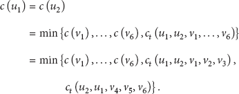
During a local sweep, two nodes are localized via five to six reference nodes. Figure 4(b) shows an example for local sweep within three-hop neighborhood (in local sweep with two-hop neighborhood, five reference nodes are used; it is just like the case when $v_2$ and $v_6$ are the same node). In this example both $u_1$ and $u_2$ can be localized via six references $v_1,\dots ,v_6$ . Since the positions of $u_1$ and $u_2$ depend on each other, $c(u_1)=c(u_2)$ . The confidence of trilateration $c_t(u_1,u_2,v_1,v_2,v_3,v_4,v_5,v_6)=\min \{c_t(u_1,u_2,v_1,v_2,v_3),c_t(u_2,u_1,v_4,v_5,v_6)\}$ , that is, the minimum one of the confidences of two tetrahedrons ( $\Delta u_2{v}_1{v}_2{v}_3$ in red and $\Delta u_1{v}_4{v}_5{v}_6$ in blue). Then, the node confidences of $u_1$ and $u_2$ are given by the following equation:

$$\begin{array}{l}c\left(u_1\right)=c\left(u_2\right)\hfill \\ =\min \{c\left(v_1\right),\dots ,c\left(v_6\right),c_t(u_1,u_2,v_1,\dots ,v_6)\}\hfill \\ =\min \{c\left(v_1\right),\dots ,c\left(v_6\right),c_t\left(u_1,u_2,v_1,v_2,v_3\right),\hfill \\ \phantom{mmmm}{c}_t(u_2,u_1,v_4,v_5,v_6)\}.\hfill \end{array}$$

(3)

For example, assume that the confidence values of $v_1$ to $v_6$ are 0.95, 1, 0.9, 0.83, 0.85, and 0.92, and the confidence from trilaterations $c_t(u_1,u_2,v_1,v_2,v_3)=0.85$ and $c_t(u_2,u_1,v_4,v_5,v_6)=0.8$ . Then, $c(u_1)=c(u_2)=\min \{\mathrm{0.95,1},\mathrm{0.9,0.83,0.85,0.92,0.85,0.8}\}=0.8$ .

By having the definition of node confidence, we can modify all proposed methods by requiring a minimum confidence threshold α. A node v can be localized via either trilateration (Line 4 in Algorithm 2 and Line 4 in Algorithm 3) or local sweep (Line 6 and Line 9 in Algorithm 3) if and only if $c(v)\ge \alpha$ . A confidence calculation and check procedure is introduced into those lines before the node(s) can be marked as localized. If $c(v)<\alpha$ , this node needs to wait for more reference nodes (green nodes) in its neighbors. If a node is selected as an anchor (marked as black in Line 5/13 of Algorithm 1 and Line 5/14 of Algorithm 4), its confidence is set to be one.

7. Simulation Results

In order to evaluate the performance of proposed methods, extensive simulations are conducted on random generated 3D ocean sensor networks. In all simulations, $100~1050$ sensor nodes are randomly deployed within a $2000\hspace{0.17em}\text{m}\times 2000\hspace{0.17em}\text{m}\times 2000\hspace{0.17em}\text{m}$ cubic region. The sensing range r of each node is set to be $300\hspace{0.17em}\text{m}$ ; that is, if the distance between two nodes is less than or equal to $300\hspace{0.17em}\text{m}$ , we assume that there is a distance measurement between them. The sensing range of the sea surface vessel is set as $900\hspace{0.17em}\text{m}$ ; that is, all sensor nodes within $900\hspace{0.17em}\text{m}$ depth are the shallow sensor nodes. A certain number of sensor nodes' coordinates are generated within the cubic region. Then, using all the shallow nodes as anchors and trilateration, all sensor nodes which cannot be localized will be deleted. We only consider all sensor nodes which are localizable when all shallow sensor nodes are set as anchors. For each set of simulations, we perform the simulations for 100 times (i.e., over 100 random networks) and report the average results over these 100 simulations. We implement the following three proposed methods: Greedy-Trilateration (Algorithms 1 and 2), Greedy-LocalSweep (Algorithms 1 and 3), and Greedy-TravelDist (Algorithms 2 and 4). In addition, we also test a random method Greedy-Random. In Greedy-Random, trilateration is recursively used to localize as many nodes as possible, and when there is no more nodes that can be localized, a random node is picked to be the next anchor. This procedure is repeated until every node is localized. In the following sections, we will test these four methods in different experiments.

7.1. Experiments for MC3DLP-1

In MC3DLP-1, our objective is to minimize the number of anchors. Figure 5(a) shows the total number of anchors selected by each algorithm. It is obvious that the less anchor nodes selected the better. Among all methods, the random method needs the most number of anchors. Greedy-LocalSweep yields the best performance, since it can localize more nodes at each step. All the greedy algorithms will converge after the sensor nodes become denser. Overall, the total number of anchors first increases with the node number and then drops down sharply around 400. Figure 5(b) shows the percentage of anchors to the total number of shallow sensor nodes. Clearly, the percentage of anchors drops while the number of sensors increases. When the sensor network is sparse, most of the shallow sensors have to be anchors. When the sensor network is very dense, only very small percentage of nodes needs to be anchors. This shows that our proposed algorithms can achieve better performances for large-scale 3D sensor networks.

Figure 5

Performances of different methods for MC3DLP-1 and MC3DLP-2.

We also study the impact of sensing range r on the performances of our proposed algorithms. Figure 6(a) shows the results of Greedy-Trilateration when the sensing range increases from $200\hspace{0.17em}\text{m}$ to $500\hspace{0.17em}\text{m}$ . Obviously, with smaller sensing ranges, our algorithm needs more anchors to locate all sensor nodes. Note that, with $r=200\hspace{0.17em}\text{m}$ , the number of anchors keeps increasing with the increasing number of sensors. However, for most cases, the number of anchors first increases with the node number and then drops down after certain critical value. If the sensing range is large enough, such as $500\hspace{0.17em}\text{m}$ , the number of anchors decreases with the increasing number of nodes and approaches rapidly a minimum level. This is reasonable, since most of the sensors are already localizable by just a few anchors. More anchors are unnecessary.

Figure 6

Performances of (a, b) Greedy-Trilateration and (c, d) Greedy-TravelDist with different sensing ranges r (from 200 m to 500 m).

7.2. Experiments for MC3DLP-2

In MC3DLP-2, we aim to minimize the traveling distance of the surface vessel due to high cost of traveling in the sea. We use the same setting with experiments for MC3DLP-1. Figure 5(c) shows the traveling distance of each algorithm based on the visiting sequence of the greedy algorithms (i.e., the ordering of selected anchor nodes). As expected, fewer anchor nodes result in shorter traveling distance. However, the random method has much longer traveling distance than other greedy methods. Moreover, Greedy-TravelDist has similar performances as Greedy-Trilateration. It means that the anchor number plays more important role in the randomly deployed network. This may be due to the similar distance among sensor nodes in a uniformly random deployment.

As discussed in Section 5.2, we can also use the existing TSP algorithm to optimize the traveling distance of each algorithm. We feed the positions of all selected anchors in a genetic TSP algorithm and use the ouput path as the course of the surface vessel. Figure 5(d) shows the results. Roughly, the total traveling distances are shortened to half of the original ones. Moreover, the difference between the random method and other greedy methods becomes smaller and Greedy-LocalSweep still yields the best result in terms of traveling distance.

Figures 6(b)–6(d) also show the performances of Greedy-Trilateration and Greedy-TravelDist when r changes from $200\hspace{0.17em}\text{m}$ to $500\hspace{0.17em}\text{m}$ . The conclusions are similar to those from Figure 6(a).

7.3. Experiments for MC3DLP with Errors

Lastly, we consider the MC3DLP problem under measurement errors. Similar to [25], we introduce a zero mean Gaussian noise $N(0,{\sigma }^2)$ to the distance measurements. In our simulations, we let $\sigma =2$ as the default value. All proposed algorithms now must consider the nodes' confidences during the localization process. As explained in Section 6, a node is localized only when its confidence $c(v)\ge \alpha$ where α is the confidence threshold. The location of the localized node is calculated using the least square estimation, since it cannot be absolutely solved due to measurement errors. In the following experiments, we also measure the location errors of each algorithm in addition to the number of selected anchors. Here, the localization error is defined as the average distance from the estimated locations to the actual locations.

( 1) The Impact of Confidence Threshold. We first study the impact of confidence threshold α by changing its value from 0.0 to 1.0. Note that when $\alpha =0.0$ , all methods do not consider the node confidence at all during the localization process. Due to space limit, we only show the results of Greedy-Random and Greedy-Trilateration in Figures 7 and 8, respectively. As expected, more anchors are needed when confidence threshold increases (as shown in Figures 7(a) and 8(a)) because higher threshold means stricter selection rules for anchor nodes. Due to stricter selection rules of anchor nodes with higher confidence thresholds, the localization accuracy increases with confidence threshold as shown in Figures 7(b) and 8(b). Note that the selection of confidence threshold may limit the localization capacity. For instance, in Figure 8(b), if α is set to be 0.25, the maximum size of localized sensor set is around 400. For a network with more than 400 sensors, the localization error increases dramatically and the localization results are not reliable. However, if the value of α is large enough (such as 0.75), the portion of localizable nodes can increase with little error increases. From Figures 7(c) and 7(d) and Figures 8(c) and 8(d), we can see that the traveling distance is heavily correlated with the selected anchor number. With larger confidence threshold, less anchors are needed which lead to smaller traveling distances. TSP can still further reduce the traveling distance after greedy algorithms.

Figure 7

Performances of Greedy-Random with different confidence thresholds α (from 0.0 to 1).

Figure 8

Performances of Greedy-Trilateration with different confidence thresholds α (from 0.0 to 1).

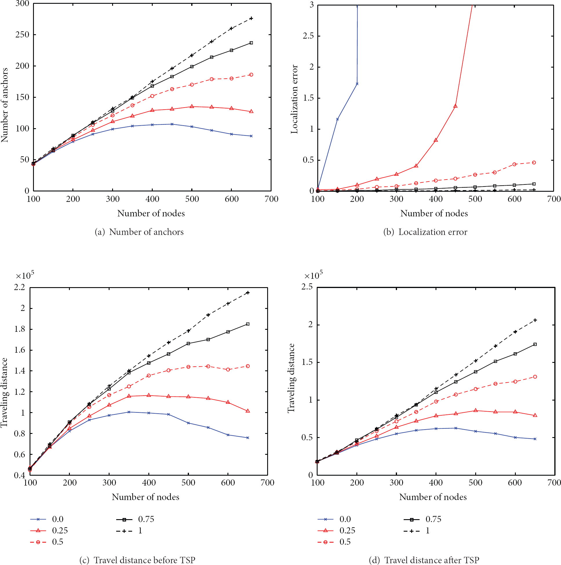
(2) Performances of Different Methods. We then study the performances of different proposed greedy algorithms. In this set of simulations, we set $\alpha =0.5$ . In this case, the anchor selection strategies will play a critical role in minimizing total number of anchor nodes. As shown in Figure 9(a), Greedy-LocalSweep and Greedy-Trilateration can achieve better performances.

Figure 9

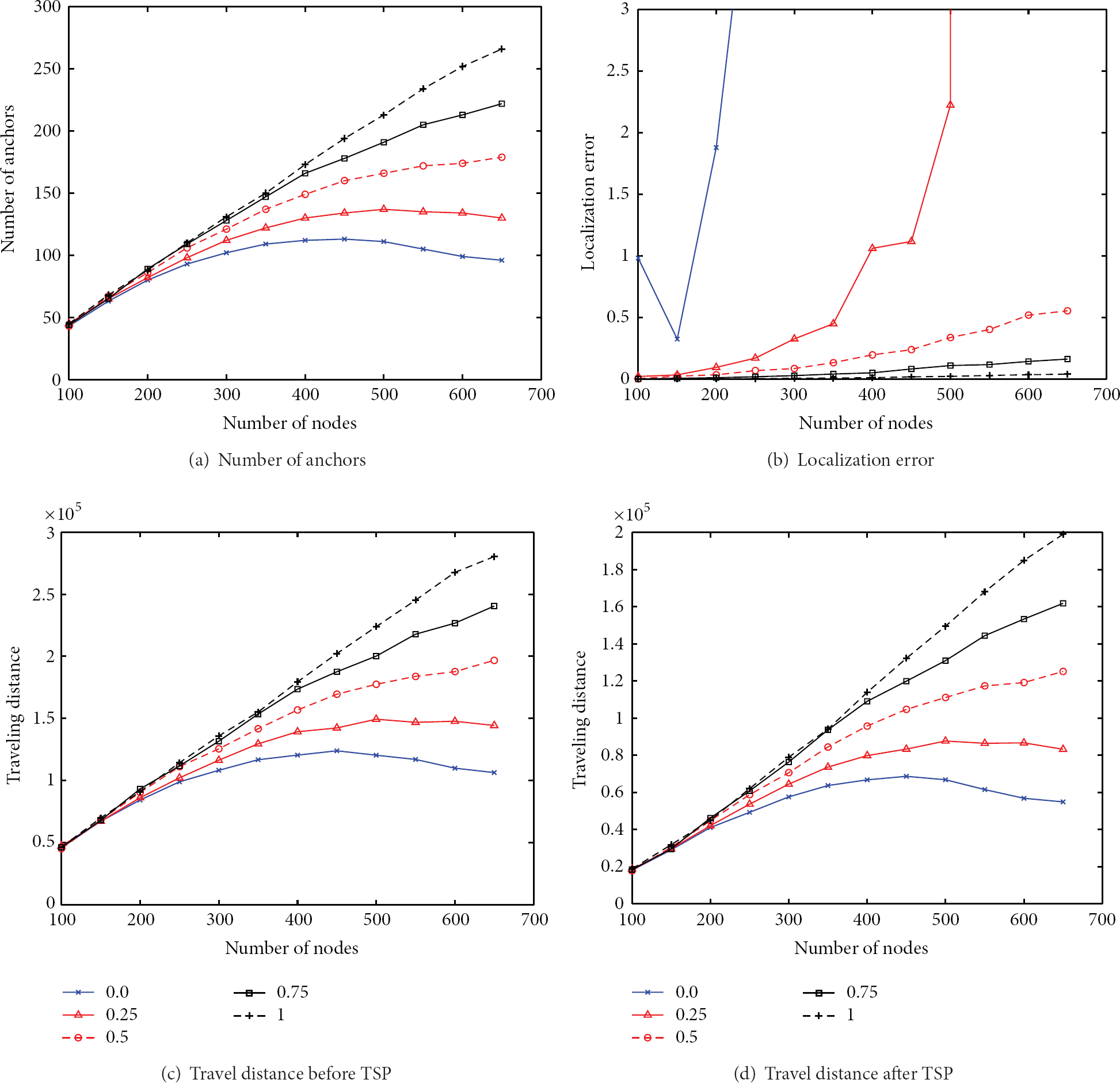
Performances of different methods with fixed $\alpha =0.5$ .

Moreover, similar to experiments for MC3DLP-1, initially, when sensor network is sparse, most of the shallow nodes have to be anchors. Gradually, as sensor network becomes denser, only small portion of shallow nodes needs to be anchors. However, localization errors induced by different methods are similar. This confirms that the confidence threshold plays more critical role in controlling localization errors as shown in Figure 9(b). In terms of travel distances, for those before TSP in Figure 9(c), it is clear that the proposed algorithms can achieve significant better performances than Greedy-Random. However, after applying TSP (as shown in Figure 9(d)), such advantages vanish mainly due to the localization errors.

(3) The Impact of Measurement Errors. At last, we investigate the influences of measurement errors in our localization problem. Here, we fix the total number of nodes as 300 and $\alpha =0.5$ . Different methods are compared for different levels of measurement errors (generated by various values of σ) as shown in Figure 10. Generally, larger value of σ leads to larger measurement errors. As expected, average localization errors increase steadily with larger measurement errors. However, the increase rate changes dramatically when $\sigma =25$ . The trend will increase and become out of control if the measurement errors keep increasing after certain threshold value.

Figure 10

Performances of different methods under different levels of errors (various values of σ).

8. Conclusion

In this paper, we extend the minimum cost localization problem to 3D ocean sensor networks in order to find the optimal anchor set to localize all sensor nodes in the network. Two versions of MC3DLP are introduced: one tries to minimize the number of anchors, while the other focuses on optimizing the traveling distance of a sea surface vessel to visit all selected anchors. Both problems are computationally challenging. We propose three different greedy algorithms to find the anchor set for a given 3D ocean sensor network. We also consider how to handle measurement errors and flip ambiguity by adopting a confidence-based approach. Extensive simulations are conducted and demonstrate the efficiency of these algorithms. We leave the problem of handling the node mobility as our future work.