Bi-Bayesian Combined Model for Two-Step Prediction of Dynamic Turning Movement Proportions at Intersections

Abstract

Short-term prediction of dynamic turning movement proportions at intersections is very important for intelligent transportation systems, but it is impossible to detect turning flows directly through current traffic surveillance devices. Existing prediction models have proved to be rather accurate in general, but not precise enough during every time interval, and can only obtain the one-step prediction. This paper first presents a Bayesian combined model to forecast the entering and exiting flows at intersections, by integrating a nonlinear regression, a moving average, and an autoregressive model. Based on the forecasted traffic flows, this paper further develops an accurate backpropagation neural network model and an efficient Kalman filtering model to predict the dynamic turning movement proportions. Using Bayesian method with both historical information and currently prediction results for error adjustment, this paper finally integrates both the above two prediction models and proposes a Bi-Bayesian combined framework to achieve both one-step and two-step predictions. A case study is implemented based on practical survey data, which are collected at an intersection in Beijing city, including both historical and current data. The reported prediction results indicate that the Bi-Bayesian combined model is rather accurate and stable for on-line applications.

1. Introduction

Origin-destination (O-D) flows represent the spatial distribution of travel demand and are very important input data for transportation planning, design, and management. The estimation of O-D flows has been studied extensively, because it is very difficult and expensive to collect O-D information through survey. In time-series cases, for example, from the aspect of real-time traffic management, we need the time-varying O-D flows, and the estimation of dynamic O-D flows turns to be much more difficult than that of static O-D flows. Furthermore, to achieve the traffic management or information service schemes in the near future periods, it is most important to predict the O-D flows in the next several time intervals.

Many models have been developed to estimate the dynamic turning movement flows (O-D flows) at intersections, for example, Cremer and Keller [1], Nihan and Davis [2, 3], Bell [4], Li and de Moor [5], and Jiao et al. [6, 7]. Based on the dynamic interrelations between time-varying input/output link flows and turning movement flows, all the above models were constructed using parameter optimization methods. These models are rather effective for real-time turning flows estimation; however, they are helpless for prediction.

Fortunately, to address the forecasting problem, as well as more efficient real-time estimation, another group of researches falls within the scope of state space formulations, and these models have been constructed using Kalman filtering method. Okutani [8] first employed a Kalman filtering method to estimate the dynamic O-D flows for freeway segments. Along the same line, many state space models have been developed using Kalman filtering technique, for example, Ashok and Ben-Akiva [9, 10], Bierlaire and Crittin [11], Lin and Chang [12], Li et al. [13], and Lou and Yin [14]. All these models are applicable for freeway segments or general road network and have proved to be rather accurate and efficient for real-time O-D estimation. Jiao et al. [15] further proposed a Bayesian combined framework integrating a Kalman filtering model and a backpropagation neural network model to estimate dynamic O-D flows at intersections. Due to the inherent one-step forecasting capability of Kalman filtering, all these models can also predict the dynamic O-D flows during the next time interval. However, they are helpless for prediction of more intervals.

More recently, Nie and Zhang [16] estimated the dynamic network O-D flows using variational inequality method. Lu et al. [17] also proposed a single-level nonlinear estimation model. Considering the constraints of dynamic user equilibrium, these models are rather accurate and are applicable for congested traffic conditions. However, similar to the parameter optimization methods, they are helpless for prediction of dynamic O-D flows in the future intervals.

With the development of short-term traffic prediction, the link traffic flows can be forecasted rather accurately. Many models have been developed, such as the artificial neural network [18], the Kalman filtering [19], and nonparametric regression [20]. Using these methods, we can forecast the entering and exiting flows at intersections during the next interval and then predict the corresponding turning movement flows. Furthermore, with the natural one-step forecasting ability of Kalman filtering, we can further predict the turning movement flows during the second interval ahead.

Meanwhile, existing researches show that the forecasted traffic flows, as well as the estimated and predicted dynamic turning movements, often fluctuate within a range around the actual values. One possible approach to deal with this problem is to design a combined model integrating multiple models together and to adjust the weight of each model automatically based on the forecasting errors. Such combined methods have been employed in existing short-term traffic forecast models, for example, Zheng et al. [21] and Dong et al. [22]. They have used Bayesian theorem [23] to construct the combined prediction models. Using a similar approach, we can improve the accuracy and stability of the forecasted entering and exiting flows, as well as the estimated and predicted turning movement flows.

One key feature of this paper is to forecast the entering and exiting flows at intersections using short-term traffic forecast methods and to construct a two-step prediction model of dynamic turning movement proportions. The second key feature is to integrate several different traffic forecasting models, as well as several different dynamic turning movement prediction models, and to present a bi-Bayesian combined model framework to predict the turning movement proportions at intersections.

The rest of the paper is organized as follows. Section 2 illustrates the basic problem statement and symbol explanations. Section 3 presents a Bayesian combined model to forecast the entering and exiting flows at intersections by integrating a nonlinear regression model, a moving average model, and an autoregressive model. Section 4 proposes a Bayesian combined model to predict the dynamic turning movement proportions by integrating a backpropagation (BP) neural network model and a revised Kalman filtering (KF) model. Both the above models constitute the bi-Bayesian combined model together. Section 5 illustrates the evaluation results of practical case study. Conclusions are given in the last section.

2. Problem Statement and Symbol Explanations

A typical intersection is illustrated in Figure 1. The number of entering approaches is r, and the number of exiting approaches is s.

Figure 1:

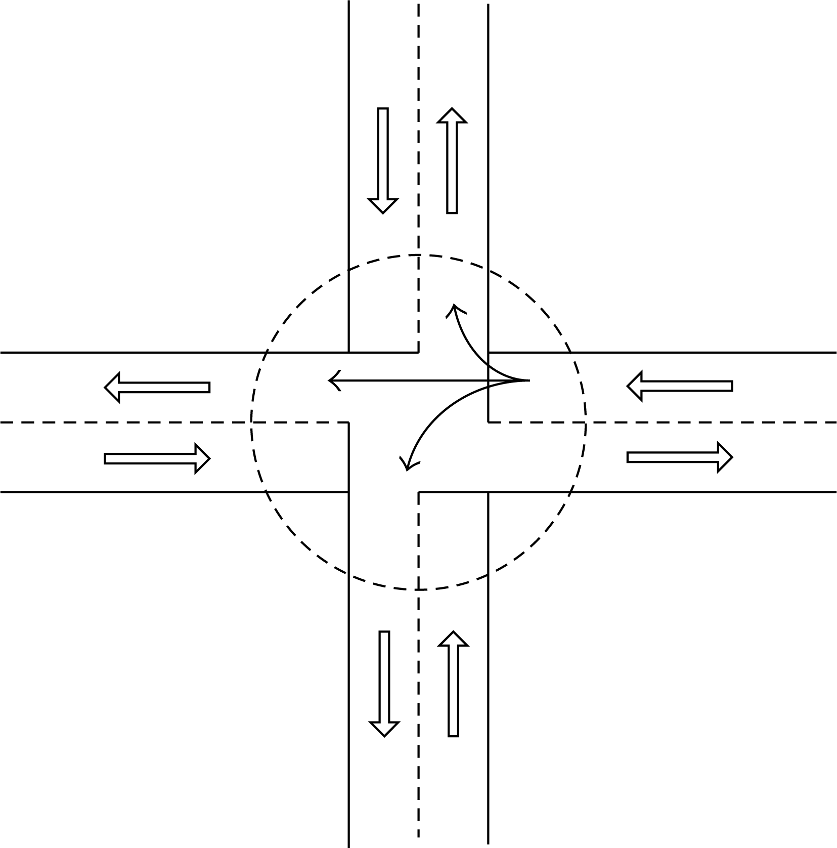
A typical intersection.

Some symbols are denoted as follows for convenient representation:

• U _i (k): arriving link flows at approach i during interval k, i = 1, 2,…, r;

• V _j (k): exiting link flows at approach j during interval k, j = 1, 2,…, s;

• F _ij (k): turning movement flows from approach i to approach j; it is actually the dynamic O-D flows at intersections;

• C _ij (k): turning split during interval k, that is, turning movement proportion to be predicted; obviously, C _ij (k) = F _ij (k)/U _i (k).

From the inherent constraints of turning movement proportions, as well as the interrelations between entering and exiting flows, we get the following basic equations:

$\mathrm{0}\le C_{ij}\left(k\right)\le \mathrm{1},$

(1)

Additionally, we use the superscript “NLR” to denote the specific variables in the nonlinear regression model, “MA” to indicate the moving average model, “AR” to show the autoregressive model, “BP” to denote the BP neural network model, “KF” to indicate the KF model, and “H” to show the historical data.

Using the above symbols, the key problem of this paper is stated as: how to predict the dynamic turning movement proportions C _ij (k) in the next one and two intervals from the detected time-series of link flows in the past and current periods.

3. Bayesian Combined Model for Entering and Exiting Flows Forecast

This paper adopts the nonlinear regression (NLR), moving average (MA), and autoregressive (AR) methods to forecast the entering and exiting flows, respectively. The basic form of the combined model is represented as

${\displaystyle \sum }_j{C}_{ij}\left(k\right)=\mathrm{1},$

(2)

where x^NLR is the forecasting result of entering or exiting flow from NLR model, x^MA is the forecasting result from MA model, x^AR is the forecasting result from AR model, W^NLR, W^MA, and W^AR are the corresponding weights, respectively.

Based on many attempts, a power function is decided in the NLR model to track the dynamics of time-varying entering and exiting flows, and a moving average of the recent 3 intervals is selected in the weighted MA model.

For x^AR, this paper adopts the AR model based on the partial autocorrelation analysis of detected link flows. As shown in Box et al. [24], a p-rank AR model is formulated below to forecast the link flows:

$V_j\left(k\right)={\displaystyle \sum }_{i\ne j}{U}_i\left(k\right)C_{ij}\left(k\right).$

(3)

where x^AR(k + 1) is the forecast result of AR model during the next time interval in the future, k is the current time interval, k–1 is the previous time interval, p is the rank of the AR model, and γ _i (i = 1, 2,…, p) is the coefficient of the AR model.

To improve the accuracy and stability of the forecast, we further integrate the above 3 forecasting models into a combined structure, with the updating flow shown in Figure 2.

Figure 2:

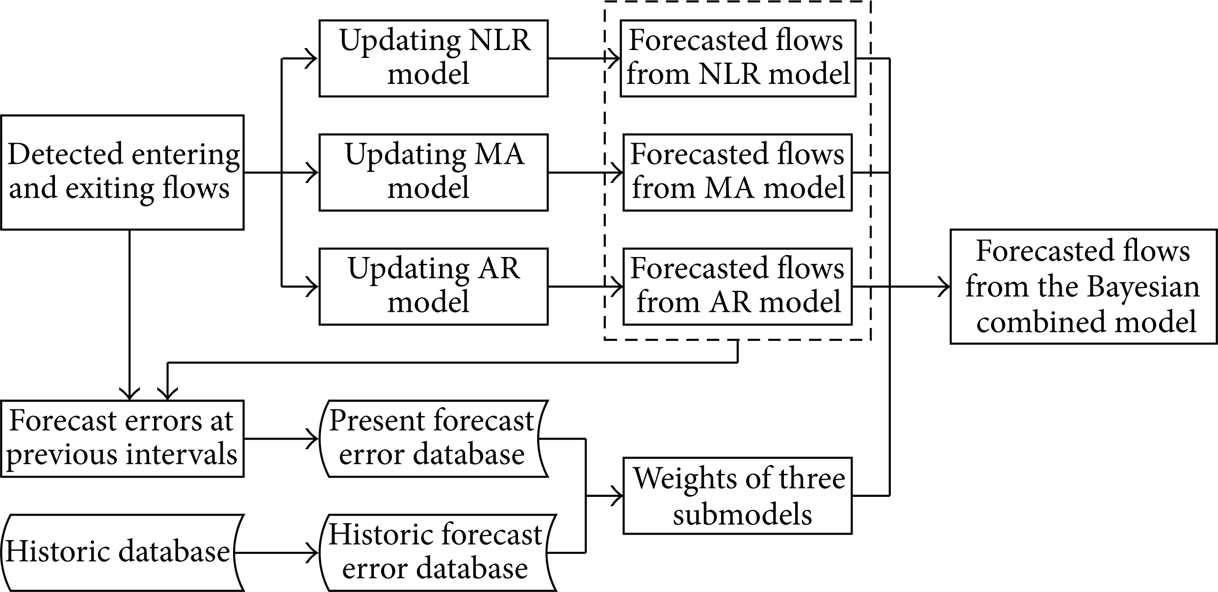
Updating flow of the Bayesian combined forecast for entering and exiting flows.

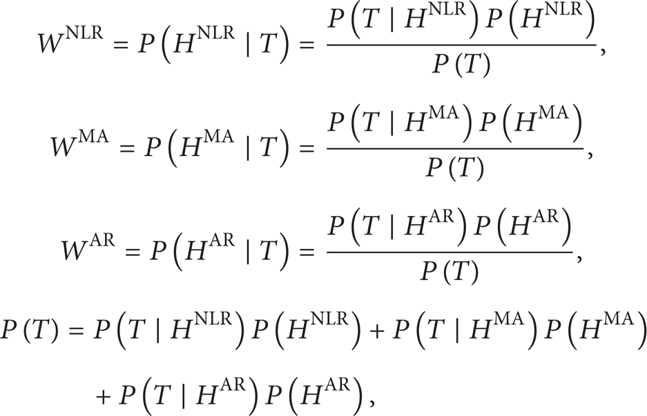
As shown in Figure 2 and (4), to reflect the influences of historical information, we first formulate the prior probabilities of NLR, MA, and AR models, respectively, as follows:

$x=W^{\text{NLR}}{x}^{\text{NLR}}+W^{\text{MA}}{x}^{\text{MA}}+W^{\text{AR}}{x}^{\text{AR}},$

(4)

where $P\left(\hspace{0.17em}\right)$ is a choice probability; P(H^NLR), P(H^MA), and P(H^AR) denote the prior probabilities to choose NLR, MA, and AR models, respectively; HM^NLR, HM^MA, and HM^AR indicate the historical mean absolute percentage errors (MAPE) of NLR, MA, and AR models, respectively. Here the MAPEs of three forecasting models are extracted from the historical forecast error database, which includes both historical predicted and actual link flows.

Using similar methods, we further formulate the following equations to express the influences of present forecast errors:

$x^{\text{AR}}\left(k+\mathrm{1}\right)={\gamma }_{\mathrm{1}}{x}^{\text{AR}}\left(k\right)+{\gamma }_{\mathrm{2}}{x}^{\text{AR}}\left(k-\mathrm{1}\right)+\cdots +{\gamma }_p{x}^{\text{AR}}\left(k-p+\mathrm{1}\right),$

(5)

where $P\left(T\mid H^{\text{NLR}}\right)$ , $P\left(T\mid H^{\text{MA}}\right)$ , and $P\left(T\mid H^{\text{AR}}\right)$ denote the probabilities to get present prediction T using historical NLR model H^NLR, MA model H^MA, and AR model H^AR, respectively, and M^NLR, M^MA, and M^AR indicate the current MAPEs of NLR, MA, and AR models, respectively. Here the MAPEs of three submodels are extracted from the previous 5 intervals, and they update with the forecasting process of the Bayesian combined model.

The weight of each submodel, that is, the posterior probability [23], is then formulated as follows:

$\begin{array}{c}P\left(H^{\text{NLR}}\right)=\left\{\begin{array}{cc}\mathrm{1}-\text{H}{\text{M}}^{\text{NLR}},\hfill & \left(\text{H}{\text{M}}^{\text{NLR}}<\mathrm{1}\right),\hfill \\ \mathrm{0},\hfill & \left(\text{H}{\text{M}}^{\text{NLR}}\ge \mathrm{1}\right),\hfill \end{array}\right)\\ P\left(H^{\text{MA}}\right)=\left\{\begin{array}{cc}\mathrm{1}-\text{H}{\text{M}}^{\text{MA}},\hfill & \left(\text{H}{\text{M}}^{\text{MA}}<\mathrm{1}\right),\hfill \\ \mathrm{0},\hfill & \left(\text{H}{\text{M}}^{\text{MA}}\ge \mathrm{1}\right),\hfill \end{array}\right)\\ P\left(H^{\text{AR}}\right)=\left\{\begin{array}{cc}\mathrm{1}-\text{H}{\text{M}}^{\text{AR}},\hfill & \left(\text{H}{\text{M}}^{\text{AR}}<\mathrm{1}\right),\hfill \\ \mathrm{0},\hfill & \left(\text{H}{\text{M}}^{\text{AR}}\ge \mathrm{1}\right),\hfill \end{array}\right)\end{array}$

(6)

where $P(H^{\text{NLR}}\mid T)$ , $P(H^{\text{MA}}\mid T)$ , and $P(H^{\text{AR}}\mid T)$ are the posterior probabilities of NLR, MA, and AR models, respectively. Actually they are equivalent to the weights of each submodel.

Using (4) and (8), one can achieve the final forecast results of entering and exiting flows at intersections, which are most important bases for the prediction of dynamic turning movement proportions.

4. Bayesian Combined Model for Dynamic Turning Movement Proportions Prediction

4.1. BP Neural Network Prediction

This paper first designs a BP neural network to forecast the dynamic turning movement proportions, as illustrated in Figure 3. A similar approach is described in our previous work [15]; however, it has not been applied to predict the future intersection turning fractions but just to estimate such information in real-time.

Figure 3:

BP neural network prediction framework.

The BP neural network model consists of three layers.

1. Input layer: there are three neurons in the input layer in this paper, which are corresponding to the link flows detected at the upstream lanes of the entering approach. Additionally, the number of neurons is decided by the number of detectors at upstream lanes.

2. Hidden layer: 15 neurons are used in the hidden layer based on many experiments. To get output results with the range [0, 1] according to (1), we employ the logarithmic sigmoid transfer function in this layer.

3. Output layer: there are three neurons in this layer, which are corresponding to the turning flows of three directions, that is, left-turn, go straight, and right-turn. Here we employ the linear transfer function directly.

As for the data in the BP neural network model, historical information, including detected link counts and surveyed actual turning proportions, is employed to train the model; current information, that is, detected link counts, is used to forecast the turning proportions.

To accelerate the training process, as well as arrive at the globally optimal solution, we introduce the self-adaptive learning rate into the traditional BP neural network method, together with the gradient descent with momentum approach. A similar algorithm has been reported in [15], and we just borrow it directly for the purpose of dynamic turning movement proportions prediction.

We code the above algorithm using Matlab platform.

4.2. KF Prediction

Furthermore, this paper constructs a KF model to forecast the time-varying turning proportions for higher efficiency. In this model, the dynamic turning fraction C _ij (k) is employed as the state variable.

Following are the state transition equation and measurement equation:

$\begin{array}{c}P\left(T\mid H^{\text{NLR}}\right)=\left\{\begin{array}{cc}\mathrm{1}-M^{\text{NLR}},\hfill & \left(M^{\text{NLR}}<\mathrm{1}\right),\hfill \\ \mathrm{0},\hfill & \left(M^{\text{NLR}}\ge \mathrm{1}\right),\hfill \end{array}\right)\\ P\left(T\mid H^{\text{MA}}\right)=\left\{\begin{array}{cc}\mathrm{1}-M^{\text{MA}},\hfill & \left(M^{\text{MA}}<\mathrm{1}\right),\hfill \\ \mathrm{0},\hfill & \left(M^{\text{MA}}\ge \mathrm{1}\right),\hfill \end{array}\right)\\ P\left(T\mid H^{\text{AR}}\right)=\left\{\begin{array}{cc}\mathrm{1}-M^{\text{AR}},\hfill & \left(M^{\text{AR}}<\mathrm{1}\right),\hfill \\ \mathrm{0},\hfill & \left(M^{\text{AR}}\ge \mathrm{1}\right),\hfill \end{array}\right)\end{array}$

(7)

where C(k) is the column vector form of turning proportion C _ij (k); accordingly, C(k + 1) is the vector of C _ij (k + 1); V(k) is the column vector form of exiting flows; U(k) is the measurement matrix, which can be achieved through arriving flows at entering legs; W(k + 1) and e(k) are the column vector form of independent random errors, representing Gauss white noises of state transition process and measurement, respectively.

The above two equations constitute the state space model together to forecast and estimate the dynamic turning fractions.

We further design an efficient sequential KF algorithm to solve the above model. In this algorithm, we replace the initial values of C _ij (k) using (11) instead of the average value 0.33:

$\begin{array}{c}{W}^{\text{NLR}}=P\left(H^{\text{NLR}}\mid T\right)=\frac{P\left(T\mid H^{\text{NLR}}\right)P\left(H^{\text{NLR}}\right)}{P\left(T\right)},\\ W^{\text{MA}}=P\left(H^{\text{MA}}\mid T\right)=\frac{P\left(T\mid H^{\text{MA}}\right)P\left(H^{\text{MA}}\right)}{P\left(T\right)},\\ W^{\text{AR}}=P\left(H^{\text{AR}}\mid T\right)=\frac{P\left(T\mid H^{\text{AR}}\right)P\left(H^{\text{AR}}\right)}{P\left(T\right)},\\ P\left(T\right)=P\left(T\mid H^{\text{NLR}}\right)P\left(H^{\text{NLR}}\right)+P\left(T\mid H^{\text{MA}}\right)P\left(H^{\text{MA}}\right)+P\left(T\mid H^{\text{AR}}\right)P\left(H^{\text{AR}}\right),\end{array}$

(8)

where Lane _ij denotes the number of lanes from entrance approach i turning to exiting approach j. If different turning directions coexist in the same lane, Lane _ij is divided into corresponding directions averagely. The convergence of the sequential KF algorithm will be accelerated due to this revision.

We also code the revised sequential KF algorithm using Matlab platform.

4.3. Bayesian Combined Prediction

We can predict the time-varying turning fractions C _ij ^BP(k) and C _ij ^KF(k), respectively, using the above BP neural network and KF models, where C _ij ^BP(k) denotes the BP neural network prediction and C _ij ^KF(k) indicates the KF prediction. To improve the accuracy and stability of the prediction, we further integrate the above two prediction models into a combined structure, and the updating mechanism of the combined model is illustrated in Figure 4, which is rather similar to Figure 2.

Figure 4:

Bayesian combined updating mechanism for prediction.

Based on the forecasted entering and exiting flows at intersections in Section 3, Figures 2 and 4 constitute a bi-Bayesian combined prediction framework for dynamic turning movement proportions together.

The detailed updating mechanism of the input data, that is, the detected and forecasted entering and exiting flows, is described in Figure 5. Here n is the total number of time intervals.

Figure 5:

Updating mechanism of entering and exiting flows.

From Figure 5, one can find out that, for each step, only link flows during the last interval are from forecast results, while flows during all previous intervals are from detected data. Therefore, the input link flows update momentarily during the prediction process.

Similar to the Bayesian combined model for entering and exiting flows forecast, we describe the model in Figure 4 as follows.

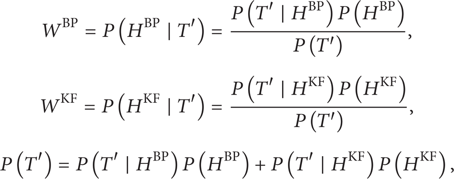
To reflect the influences of historical information, we first formulate the prior probabilities of BP neural network and KF models, respectively, as shown below:

$\mathbf{C}\left(k+\mathrm{1}\right)=\mathbf{C}\left(k\right)+\mathbf{W}\left(k+\mathrm{1}\right),$

(9)

where P(H^BP) denotes the prior probability to choose BP neural network model, HM^BP indicates the historical MAPE of BP neural network model, P(H^KF) shows the prior probability to choose KF model, and HM^KF is the historical MAPE of KF model. Here the MAPEs of BP neural network and KF models are extracted from the historical forecast error database, which includes both historical predicted and actual turning fractions.

Using similar methods, we further formulate the following equations to express the influences of present prediction errors:

$\mathbf{V}\left(k\right)=\mathbf{U}\left(k\right)*\mathbf{C}\left(k\right)+\mathbf{e}\left(k\right),$

(10)

where $P(T^{\prime }\mid H^{\text{BP}})$ denotes the probability to get present prediction T′ using historical BP neural network model H^BP, M^BP indicates the current MAPE of BP neural network model, $P(D^{\prime }\mid H^{\text{KF}})$ shows the probability to get present prediction T′ using historical KF model H^KF, and M^KF is the current MAPE of KF model. Here the MAPEs of BP neural network and KF models are extracted from the previous 5 intervals, and they update with the prediction process of the bi-Bayesian combined model.

For the current MAPEs, a most important problem worth mentioning is that the current actual turning fractions are impossible to be obtained from the traffic surveillance systems. In this paper, the Bayesian combined predictions are employed as substitutes. Furthermore, since the number of previous intervals is not enough during the starting process, the historic actual values during the corresponding intervals are used alternatively.

The weight of each submodel, that is, the posterior probability [23], is then formulated as follows:

$C_{ij}\left(\mathrm{0}\right)=\frac{\text{Lan}{\text{e}}_{ij}}{{\sum }_j^{}\text{Lan}{\text{e}}_{ij}},$

(11)

where W^BP denotes BP neural network model's weight, which is equivalent to the posterior probability $P(H^{\text{BP}}\mid T^{\prime })$ , and W^KF indicates the KF model's weight, which is equivalent to the posterior probability $P(H^{\text{KF}}\mid T^{\prime })$ .

The predicted dynamic turning movement proportions are then presented as

$\begin{array}{c}P\left(H^{\text{BP}}\right)=\left\{\begin{array}{cc}1-\text{H}{\text{M}}^{\text{BP}},\hfill & \left(\text{H}{\text{M}}^{\text{BP}}<1\right),\hfill \\ 0,\hfill & \left(\text{H}{\text{M}}^{\text{BP}}\ge 1\right),\hfill \end{array}\right)\\ P\left(H^{\text{KF}}\right)=\left\{\begin{array}{cc}1-\text{H}{\text{M}}^{\text{KF}},\hfill & \left(\text{H}{\text{M}}^{\text{KF}}<1\right),\hfill \\ 0,\hfill & \left(\text{H}{\text{M}}^{\text{KF}}\ge 1\right),\hfill \end{array}\right)\end{array}$

(12)

where ${\tilde{C}}_{ij}\left(k\right)$ is the predicted dynamic turning movement proportions from the bi-Bayesian combined model.

Using (14) to (15), one can achieve the final prediction results.

With the natural forecasting ability of BP neural network and KF models, the bi-Bayesian combined model can achieve the dynamic turning movement proportions in 3 different cases:

1. real-time estimation based on detected link flows, using only estimation ability;

2. one-step prediction based on both detected and forecasted link flows, using only estimation ability;

3. two-step prediction based on both detected and forecasted link flows, using both estimation and forecasting abilities.

5. Case Study

We applied the bi-Bayesian combined model to a practical intersection at Zhaodengyu-Pinganli west crossroad in Beijing city, China. For the convenience of description, we denote the east approach by “1,” the south approach by “2,” the west approach by “3,” and the north approach by “4”. Since the actual turning movement flows can be collected through the survey, we can verify the accuracy of the proposed prediction model.

Through a real-world survey, we obtained the time-series of link counts at all entering and exiting approaches, as well as the turning flows. To get the historical information, we conducted the survey twice from 7 am to 9 am on a Tuesday and a Wednesday, respectively, and the weather is almost the same. The Tuesday information was employed as the historical data, while the Wednesday information was used as the present data.

We first forecasted the entering and exiting flows using the Bayesian combined model based on NLR, MA, and AR methods. Furthermore, we implemented the dynamic turning movement proportions estimation and prediction using the bi-Bayesian combined model and obtained all results of the real-time estimation, one-step prediction, and two-step prediction. To explore the detailed information, we employed a 3-minute interval in the case study, and totally we had 40 intervals for each day.

A rather important thing worth mentioning is the BP neural network model. For the historical information on Tuesday, we used first 30 intervals to train the BP neural network and forecasted the results of last 10 intervals to collect the historical prediction errors. Moreover, we used all 40 intervals on Tuesday to train the model again and forecasted the results of all 40 intervals on Wednesday. The present prediction errors in the Bayesian combined model were also extracted from the forecasting results on Wednesday.

As described in Section 5, three scenarios were designed to testify the proposed model.

Scenario 1. Real-time estimation is as follows:

1. data: detected link flows;

2. result: real-time estimation of turning movement proportions;

3. model: estimation model.

Scenario 2. One-step prediction is as follows:

1. data: detected and forecasted link flows;

2. result: one-step prediction of turning movement proportions;

3. model: estimation model, updating the forecasted link flows during each estimation interval.

Scenario 3. Two-step prediction is as follows:

1. data: detected and forecasted link flows;

2. result: two-step prediction of turning movement proportions;

3. model: prediction model, updating the forecasted link flows during each prediction interval.

We take C₁₄(k), C₃₁(k), and C₄₁(k), for example, to verify the accuracy of the bi-Bayesian combined prediction model. Here all three turning directions are covered, that is, right-turn, go straight, and left-turn. We use four evaluation criteria to show the model accuracy:

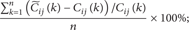
1. mean average percentage: MAPE, defined as

   $\begin{array}{c}P\left(T^{\prime }\mid H^{\text{BP}}\right)=\left\{\begin{array}{cc}1-M^{\text{BP}},\hfill & \left(M^{\text{BP}}<1\right),\hfill \\ 0,\hfill & \left(M^{\text{BP}}\ge 1\right),\hfill \end{array}\right)\\ P\left(T^{\prime }\mid H^{\text{KF}}\right)=\left\{\begin{array}{cc}1-M^{\text{KF}},\hfill & \left(M^{\text{KF}}<1\right),\hfill \\ 0,\hfill & \left(M^{\text{KF}}\ge 1\right),\hfill \end{array}\right)\end{array}$

   (13)

2. mean percentage error: MPE, defined as

   $\begin{array}{c}{W}^{\text{BP}}=P\left(H^{\text{BP}}\mid T^{\prime }\right)=\frac{P\left(T^{\prime }\mid H^{\text{BP}}\right)P\left(H^{\text{BP}}\right)}{P\left(T^{\prime }\right)},\\ W^{\text{KF}}=P\left(H^{\text{KF}}\mid T^{\prime }\right)=\frac{P\left(T^{\prime }\mid H^{\text{KF}}\right)P\left(H^{\text{KF}}\right)}{P\left(T^{\prime }\right)},\\ P\left(T^{\prime }\right)=P\left(T^{\prime }\mid H^{\text{BP}}\right)P\left(H^{\text{BP}}\right)+P\left(T^{\prime }\mid H^{\text{KF}}\right)P\left(H^{\text{KF}}\right),\end{array}$

   (14)

3. root mean square error: RMSE, defined as

   ${\tilde{C}}_{ij}\left(k\right)=W^{\text{BP}}\left(k\right)\times C_{ij}^{\text{BP}}\left(k\right)+W^{\text{KF}}\left(k\right)\times C_{ij}^{\text{KF}}\left(k\right),$

   (15)

4. normalized root mean square: NRMS, defined as

   $\frac{{\sum }_{k=1}^n\left|{\tilde{C}}_{ij}\left(k\right)-C_{ij}\left(k\right)\right|/C_{ij}\left(k\right)}{n}\times 100\%;$

   (16)
   $\frac{{\sum }_{k=1}^n\left({\tilde{C}}_{ij}\left(k\right)-C_{ij}\left(k\right)\right)/C_{ij}\left(k\right)}{n}\times 100\%;$

   (17)
   $\sqrt{\frac{{\sum }_{k=1}^n{\left[{\tilde{C}}_{ij}\left(k\right)-C_{ij}\left(k\right)\right]}^2}{n}};$

   (18)
   $\frac{\sqrt{n{\sum }_{k=1}^n{\left[{\tilde{C}}_{ij}\left(k\right)-C_{ij}\left(k\right)\right]}^2}}{{\sum }_{k=1}^n{C}_{ij}\left(k\right)}\times 100\%.$

   (19)

Here n denotes the total number of time intervals.

The evaluation indices of real-time estimation, one-step prediction, and two-step prediction are all reported in Table 1. The results of the last 30 intervals are employed in the indices statistics.

Table 1:

Statistical results of evaluation indices.

Index	C 14			C 31			C 41
	Estimate	One-step	Two-step	Estimate	One-step	Two-step	Estimate	One-step	Two-step
MAPE	31.76%	32.53%	30.01%	11.59%	10.07%	10.43%	32.96%	37.89%	34.61%
MPE	7.87%	14.78%	2.93%	10.69%	7.38%	7.38%	19.93%	22.55%	15.23%
RMSE	0.047	0.048	0.050	0.116	0.101	0.102	0.089	0.091	0.088
NRMS	34.42%	34.78%	36.33%	14.45%	12.52%	12.67%	35.58%	36.52%	35.36%

In Table 1, “estimate” denotes the real-time estimation in Scenario 1, “one-step” indicates the one-step prediction in Scenario 2, and “two-step” shows the two-step prediction in Scenario 3.

Figures 6, 7, and 8 further illustrate the above estimation and prediction results.

Figure 6:

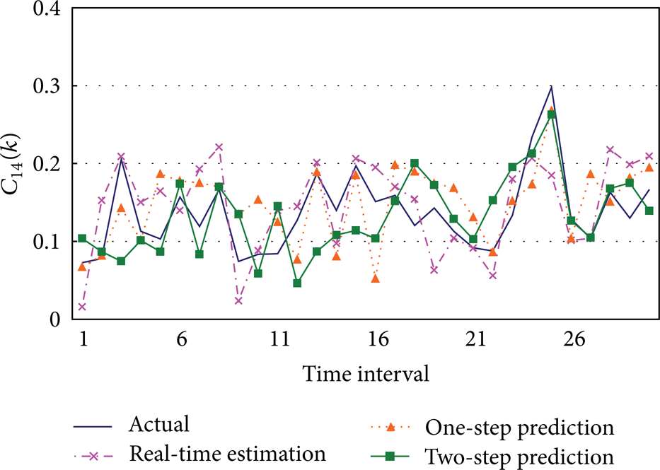
Actual versus predicted turning proportion C₁₄(k).

Figure 7:

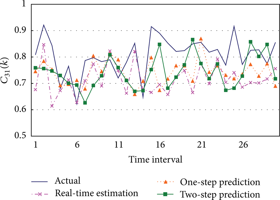
Actual versus predicted turning proportion C₃₁(k).

Figure 8:

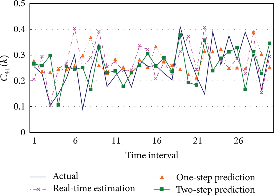
Actual versus predicted turning proportion C₄₁(k).

As expected, one can find out the following results from the case study.

1. All three groups of results are rather accurate and fluctuate within a narrow range around the actual values.

2. From the common sense, the prediction results should be less accurate than estimation results due to the errors of forecasted input flows; however, this case study shows different conclusions; that is, for some turning proportions, the estimation is more accurate than prediction, but vice versa for other turning proportions. The possible reason is that there exist errors in both estimation/prediction models and traffic flow forecast models, and in some cases these errors will cancel each other out.

3. Concerning the capability of tracking the dynamics of turning movement proportions, three scenarios achieve rather similar results again.

4. The estimation results of go straight direction are much more accurate than those of left-turn and right-turn directions, due to the rather bigger magnitudes of the go straight turning movement proportions.

6. Conclusions

This paper addresses a bi-Bayesian combined model framework concerning dynamic turning movement proportions prediction at intersections. We first present a Bayesian combined model to forecast the entering and exiting flows at intersections by integrating a nonlinear regression model, a moving average model, and an autoregressive model. Based on the detected and forecasted traffic flows, we further propose a Bayesian combined model to estimate and predict the dynamic turning movement proportions by integrating a backpropagation neural network model and a revised Kalman filtering model. Both the above Bayesian models constitute the bi-Bayesian combined model together. This bi-Bayesian combined model has three capabilities: to estimate the dynamic turning movement proportions in real-time, to obtain the one-step prediction of turning movement proportions, and to achieve the two-step prediction of turning movement proportions. The case study based on real-world data has demonstrated the accuracy and effectiveness of the proposed bi-Bayesian prediction model.

The proposed bi-Bayesian combined model for two-step prediction of dynamic turning movement proportions can be enhanced in two aspects. First, vehicles need some time to cross the intersection, especially under traffic congestion, but such travel time is neglected in this model because it is rather shorter than one time interval. Second, prediction of dynamic O-D flows in freeway corridor and road network is very important, and introduction of dynamic travel time and route choice probability will direct the model to such cases.

Conflict of Interests

The authors declare that there is no conflict of interests regarding the publication of this paper.