
Abstract
Simple rules are developed for obtaining rational bounds for two-phase frictional pressure gradient and void fraction in circular pipes. The bounds are based on turbulent-turbulent flow assumption. Both the lower and upper bounds for frictional pressure gradient are based on the separate cylinders formulation. For frictional pressure gradient, the lower bound is based on the separate cylinders formulation that uses the Blasius equation to represent the Fanning friction factor while the upper bound is based on the separate cylinders equation that represents well the Lockhart-Martinelli correlation for turbulent-turbulent flow. For void fraction, the lower bound is based on the separate cylinders formulation that uses the Blasius equation to predict the Fanning friction factor while the upper bound is based on the Butterworth relationship that represents well the Lockhart-Martinelli correlation. These two bounds are reversed in the case of liquid fraction (1-α). For frictional pressure gradient, the model is verified using published experimental data of two-phase frictional pressure gradient versus mass flux at constant mass quality. The published data include different working fluids such as R-12, R-22, and Argon at different mass qualities, different pipe diameters, and different saturation temperatures. The bounds models are also presented in a dimensionless form as two-phase frictional multiplier (ϕ l and ϕ g ) versus Lockhart-Martinelli parameter (X) for different working fluids such as R-12, R-22, and air-water and steam mixtures. For void fraction, the bounds models are verified using published experimental data of void fraction versus mass quality at constant mass flow rate. The published data include different working fluids such as steam, R-12, R-22, and R-410A at different pipe diameters, different pressures, and different mass flow rates. It is shown that the published data can be well bounded for a wide range of mass fluxes, mass qualities, pipe diameters, and saturation temperatures.
1. Introduction
In the present study, the lower and upper bounds for two-phase frictional pressure gradient and void fraction in circular pipes are developed. This approach is very useful in design and analysis, as engineers can then use the resulting average and bounding values in predictions of system performance. For example, comparisons of several two-phase flow models for the frictional pressure gradient [1] and the void fraction [2] show that no two models provide the same results for the frictional pressure gradient and the void fraction. Since all models were developed in conjunction with experimental data, which are prone to measurement error, it is reasonable to expect that any prediction is also subject to similar error. The use of bounds can alleviate some of the subjectivity of the published two-phase flow models for the frictional pressure gradient and the void fraction by providing definite limits on the value of the two-phase frictional pressure gradient and the two-phase void fraction. The approach is also useful when conducting new experiments, since it provides a reasonable envelope for the data to fall within. The bounds are intended to provide the most realistic range of data not firm absolute limits. Statistically, this is unreasonable as the bounds would be far apart. The bounds are not fit to capture all data but rather a majority of data points, as some outlying points are due to experimental error. If a vast majority of data is within the bounds, then a reasonable expectation is realistically assured.
2. Proposed Methodology
2.1. Development of Bounds on Two-Phase Frictional Pressure Gradient in Circular Pipes
In this section, rational bounds for two-phase frictional pressure gradient in circular pipes will be developed. These bounds may be used to determine the maximum and minimum values that may reasonably be expected in a two-phase flow. Further, by averaging these limiting values an acceptable prediction for the pressure gradient is obtained which is then bracketed by the bounding values:

The bounds model will be in the form of two-phase frictional pressure gradient versus mass flux at constant mass quality. The bounds model may also be presented in the form of two-phase frictional multiplier, which is often useful for calculation and comparison needs. For this reason, development of lower and upper bounds in terms of two-phase frictional multiplier (ϕ l and ϕ g ) versus the Lockhart-Martinelli parameter (X) will also be presented.
In the present study, the bounds method is based on turbulent liquid-turbulent gas assumption [1, 2]. This assumption is suitable because, in practice, both Re l and Re g are most often greater than 2000 in circular pipes. On the other hand, the assumption of laminar liquid-laminar gas is suitable for the flow in minichannels and microchannels [8] because, in practice, both Re l and Re g are most often less than 2000 in minichannels and microchannels.
Both the lower and upper bounds are based on the separate cylinders formulation [9]. The equation of the separate cylinders model [9] is

The values of n were dependent on whether the liquid and gas phases were laminar or turbulent flow. The different values of n are given in Table 1. The reasons of choosing lower and upper bounds can be explained as follows.
Values of exponent (n) for different flow types.
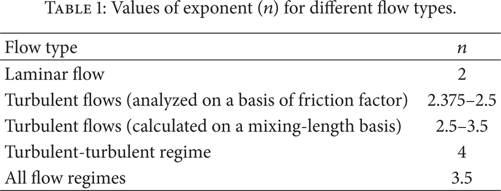
From Table 1, it is obvious that the different values of n for turbulent-turbulent flow in separate-cylinders model can be:
n = 2.375 (f = 0.079/Re0.25),
n = 2.4 (f = 0.046/Re0.2),
n = 2.5 (f = constant),
n = 3.5 (maximum value in mixing-length analysis),
n = 4 (good empirical representation of the Lockhart-Martinelli correlation [10]).
The present model is based on the minimum and maximum values of n for turbulent-turbulent flow, 2.375, and 4, respectively, from the separate-cylinders formulation [9].
Also, although the data points are in turbulent-turbulent flow, they cover different flow patterns such as stratified, wavy, slug, and annular. As the mass flow rate of the gas in two-phase flow increases, the flow pattern changes from stratified to wavy to slug to annular. As mentioned in the literature, the Lockhart-Martinelli correlation [10] has a good accuracy for annular flow pattern [11] but it has a poor accuracy (overprediction) for stratified and wavy flow pattern [12]. This is why it is taken as an upper bound. Further n = 4 as a closure constant was arbitrarily chosen to fit the data and thus accounts for interfacial effects between phases making it an upper bound, whereas n = 2.375 as a closure constant is obtained from the Blasius friction model [13] and does not account for interfacial effects and therefore represents a lower bound for the data. Faghri and Zhang [14] further commented that the advantage of the pressure drop correlations based on the separated-flow model is that they are applicable for all flow patterns. This flexibility is accompanied by low accuracy.
2.1.1. The Lower Bound
The lower bound is based on the separate cylinders formulation [9] that uses the Blasius equation [13] to represent the Fanning friction factor. Introducing the Lockhart-Martinelli parameter (X) into (2), we obtain ϕ l 2 and ϕ g 2 for turbulent-turbulent flow (n = 2.375, Table 1), respectively, as follows:

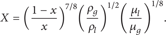
For turbulent-turbulent flow, the Lockhart-Martinelli parameter (X) can be expressed as [15]
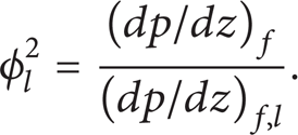
The Lockhart-Martinelli expression for the two-phase frictional multiplier (ϕ l 2) is given by
The single-phase liquid frictional pressure gradient can be related to the Fanning friction factor in terms of mass flux and mass quality for liquid flowing alone as follows:
For turbulent-turbulent flow, the Fanning friction factor is defined using the Blasius equation [13] as follows:

The Reynolds number equation can be expressed in terms of mass flux and mass quality for liquid flowing alone as

Using (3) and (5)–(9), we obtain

2.1.2. The Upper Bound
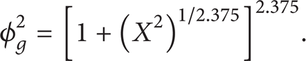
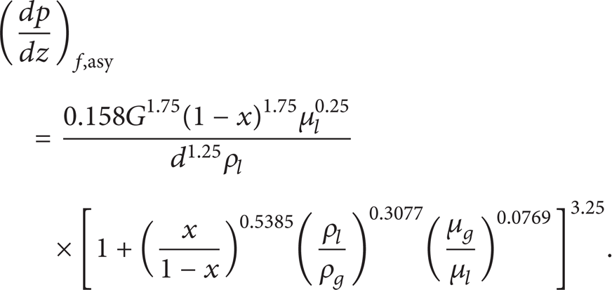
The upper bound is based on the separate cylinders formulation [9] that uses an equation that represents well the Lockhart-Martinelli correlation for turbulent-turbulent flow. The equation of the upper bound is similar to the lower bound case except for the definitions of ϕ l 2 and ϕ g 2. Introducing the Lockhart-Martinelli parameter (X) into (2), we obtain ϕ l 2 and ϕ g 2 for turbulent-turbulent flow (n = 4, Table 1), respectively, as follows:

Equations (11) and (12) represent well the Lockhart-Martinelli correlation [10] for turbulent-turbulent flow. Using (11) and (5)–(9), we obtain

2.1.3. Mean Model
A simple model may be developed by averaging the two bounds. This is defined as follows:

or

Otherwise the more accurate asymptotic model [16] should be used as follows:
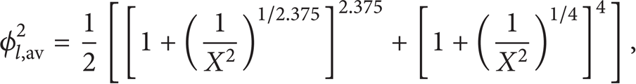
or

2.2. Development of Bounds on Two-Phase Void Fraction in Circular Pipes
In this section, rational bounds for two-phase void fraction in circular pipes will be developed. These bounds may be used to determine the maximum and minimum values that may reasonably be expected in a two-phase flow. Further, by averaging these limiting values an acceptable prediction for the void fraction is obtained which is then bracketed by the bounding values:

The bounds model will be in the form of two-phase void fraction against mass quality at constant mass flow rate. The bounds model may also be presented in the form of void fraction against the Lockhart-Martinelli parameter (X).
For the case of large circular pipes, the bounds method is based on turbulent liquid-turbulent gas assumption [1, 2]. This assumption is suitable because, in practice, both Re l and Re g are most often greater than 2000 in large circular pipes.
2.2.1. The Lower Bound
The lower bound is based on the separate cylinders formulation [9] for turbulent-turbulent flow that uses the Blasius equation [13] to predict the Fanning friction factor. Using the separate cylinders analysis [9] and introducing the Blasius equation [13] to represent the Fanning friction factor for turbulent-turbulent flow, α can be expressed as follows:

Substituting (5) into (21), we obtain

2.2.2. The Upper Bound
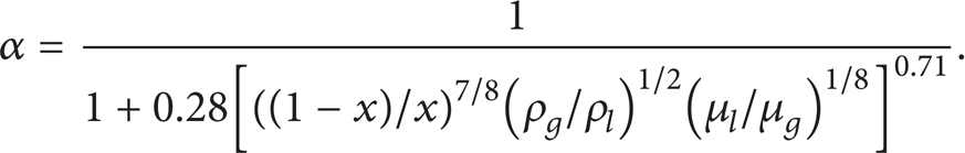
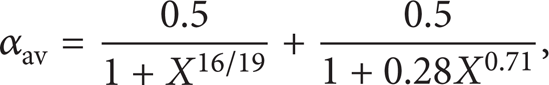
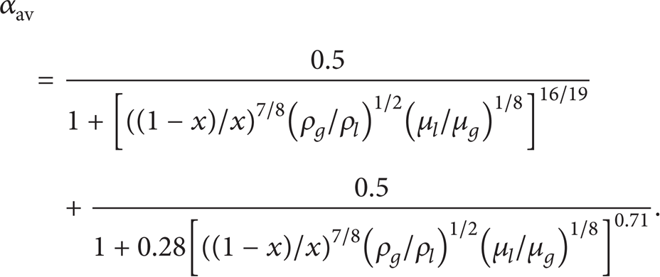
In order to make the bounds model tight and present it in the form of void fraction (α) against the Lockhart-Martinelli parameter (X), the Lockhart-Martinelli correlation [10] is chosen to represent the upper bound although the homogeneous model gives higher prediction of the void fraction (α) than the Lockhart-Martinelli correlation at the same mass quality (x) except at low values of the mass quality (x). Butterworth [17] represented the Lockhart-Martinelli correlation [10] by the relation:
Substituting (5) into (23), we obtain
Since (1-α) represents the liquid fraction, the lower and upper bounds are reversed in the case of liquid fraction data.
2.2.3. Mean Model
A simple model may be developed by averaging the two bounds. This is defined as follows:

or


3. Results and Discussion
For frictional pressure gradient, examples of two-phase frictional pressure gradient versus mass flux at constant mass quality from published experimental studies are presented to show the advantages of the bounds models. The published data include different working fluids such as R-12, R-22, and Argon at different mass qualities with different pipe diameters. Also, examples of two-phase frictional multiplier (ϕ l and ϕ g ) versus Lockhart-Martinelli parameter (X) using published data of different working fluids such as R-12, R-22, and air-water and steam from other experimental work are presented to validate the bounds model in dimensionless form.
For void fraction, examples of two-phase void fraction versus mass quality at constant mass flow rate from published experimental studies are presented to show features of the bounds. The published data include different working fluids such as steam, R-12, R-22, and R-410A at different pipe diameters, different pressures, and different mass flow rates. Also, the model is verified using published experimental data of void fraction (α) and liquid fraction (1-α) versus the Lockhart-Martinelli parameter (X) for different working fluids such as R-12, R-22, and air-water mixtures in turbulent-turbulent flow.
3.1. Two-Phase Frictional Pressure Gradient
Figures 1–4 show the frictional pressure gradient versus mass flux in turbulent-turbulent flow. Equation (10) represents the lower bound and (13) represents the upper bound, while (16) represents the average. Figure 1 compares the present approach with Bandel's data [3] for R-12 flow at x = 0.3 and T s = 0°C in a smooth horizontal pipe at d = 14 mm. Figure 2 compares the present approach with Hashizume's data [4] for R-12 flow at x = 0.8 and T s = 50°C in a smooth horizontal pipe at d = 10 mm. Figure 3 compares the present approach with Hashizume's data [4] for R-22 flow at x = 0.8 and T s = 39°C in a smooth horizontal pipe at d = 10 mm. Figure 4 compares the present approach with Müller-Steinhagen's data [5] for Argon flow at x = 0.4 and reduced pressure of 0.188 in a smooth horizontal pipe at d = 14 mm. From Figures 1–4, it can be seen that the published data can be well bounded. In Figures 1–4, the mean model predicts the published data with the root mean square (RMS) error of 26.41%, 8.62%, 11.23%, and 21.42%, respectively, while the asymptotic model, (19), gives the root mean square (RMS) error of 29.67%, 10.65%, 8.34%, and 15.75%, respectively. From Figures 1–4, it can be seen that the bounds on two-phase frictional pressure gradient in circular pipes are good indicators in experiments for establishing the validity of test results and other physical issues.
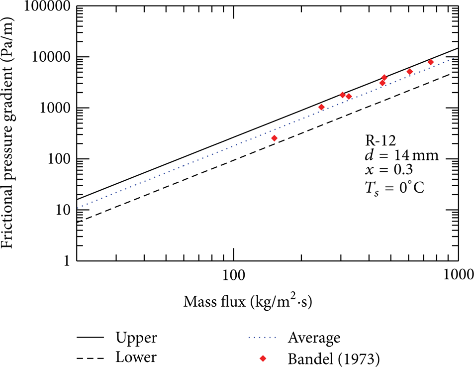
Comparison of the present model with Bandel's data [3].

Comparison of the present model with Hashizume's data [4].
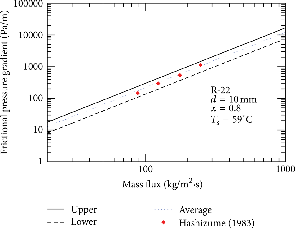
Comparison of the present model with Hashizume's data [4].

Comparison of the model with Müller-Steinhagen's data [5].
3.2. ϕ l and ϕ g versus Lockhart-Martinelli Parameter (X)
Figure 5 shows ϕ l versus Lockhart-Martinelli parameter (X) for turbulent-turbulent flow. Equation (3) represents the lower bound and (11) represents the upper bound, while (14) represents the average. Figure 5 compares the present model with the data sets of Hashizume's data [4] for R-12 flow in a smooth horizontal pipe of d = 10 mm at T s = 20°C and x = 0.1, 0.3, 0.5, and 0.8, Hashizume's data [4] for R-22 flow in a smooth horizontal pipe of d = 10 mm at T s = 20°C and x = 0.1, 0.3, 0.5, and 0.8, Govier and Omer's data [18] for air-water mixtures in a smooth horizontal pipe of 1.026 in (26.06 mm) diameter, and Janssen and Kervinen's data [19] for steam-water flow in a smooth horizontal pipe at a pressure of 1 066 psia (73.5 bar) and d = 0.742 in (18.85 mm) for G = 1.68 × 10⁶ lbm/ft2·hr (2 278 kg/m2·s). The mean model predicts the published data of ϕ l with the root mean square (RMS) error of 14.41%, 21.47%, 16.19%, and 18.7%, respectively, while the asymptotic model, (17), gives the root mean square (RMS) error of 10.8%, 16.68%, 19.87%, and 12.9%, respectively. From Figure 5, it is clear that the bounds contain a vast majority of the data.

ϕ l versus X for different sets of data.
Figure 6 shows ϕ g versus Lockhart-Martinelli parameter (X) for turbulent-turbulent flow. Equation (4) represents the lower bound and (12) represents the upper bound, while (15) represents the average. Figure 6 compares the present model with the data sets of Cicchitti et al.'s data [20] for adiabatic flow of steam in a smooth pipe of 5.1 mm diameter at a pressure of 30–60 kg/cm2 (29.4–58.8) bar and Cheremisinoff and Davis's [21] for stratified flow of air-water mixtures in a smooth horizontal pipe of 63.5 mm diameter. Cicchitti et al. [20] mentioned that their steam data for turbulent-turbulent flow (ϕ g versus X) fall in the strip bounded by the Martinelli and Nelson lines [22] drawn up for atmospheric and critical pressures. The advantages of the present bound models over the Martinelli and Nelson lines [22] at atmospheric and critical pressures are as follows.
The Martinelli and Nelson lines [22] at atmospheric and critical pressures were presented in a graphical manner while the present bound models are presented in the form of simple equations.
The Martinelli and Nelson lines [22] at atmospheric and critical pressures can be used only when steam is the working fluid while the present bound models can be used for different working fluids as in Figure 6.
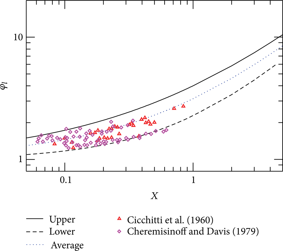
ϕ g versus X for different sets of data.
The mean model predicts the published data of ϕ g with the root mean square (RMS) error of 12.84% and 22.03%, respectively, while the asymptotic model, (18), gives the root mean square (RMS) error of 9.56% and 18.51%, respectively. From Figure 6, It is clear that the bounds contain a vast majority of the data.
3.3. Two-Phase Void Fraction
Figures 7–10 show the void fraction versus mass quality. Equation (22) represents the lower bound and (24) represents the upper bound while (26) represents the average. Figure 7 compares the present model with Larson's data [6] for adiabatic flow of steam-water mixture at p s = 1000 psia (6 894.74 kPa). Figure 8 compares the present model with Hashizume's data [4] for R-12 flow at T s = 50°C and m = 25, 35, 50, 70, and 100 kg/hr, respectively, in a smooth horizontal pipe at d = 10 mm. Figure 9 compares the present model with Hashizume's data [4] for R-22 flow at T s = 39°C and m = 25, 35, 50, 70, and 100 kg/hr, respectively, in a smooth horizontal pipe at d = 10 mm. Figure 10 compares the present model with Wojtan et al.'s data [7] R-410A flow at T s = 5°C and G = 70, 150, 200, and 300 kg/m2·s, respectively, in a smooth horizontal pipe at d = 5/8 in. (15.875 mm). In Figures 7–10, the mean model predicts the published data of α with the root mean square (RMS) error of 12.17%, 9.04%, 7.39%, and 26.86%, respectively. In Figure 10, if the two lower points at G = 70 kg/m2·s are not included, RMS will be 10.6% instead of 26.86%. From Figures 7–10, it can be seen that the bounds on two-phase void fraction in circular pipes are good indicators in experiments for establishing the validity of test results and other physical issues.
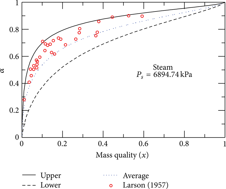
Comparison of the present model with Larson's data [6].
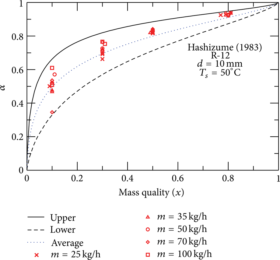
Comparison of the present model with Hashizume's data [4].

Comparison of the present model with Hashizume's data [4].

Comparison of the present model with Wojtan et al's data [7].
3.4. α and
versus Lockhart-Martinelli Parameter (X)
Figure 11 shows α versus Lockhart-Martinelli parameter (X) for turbulent-turbulent flow. Equation (21) represents the lower bound and (23) represents the upper bound, while (25) represents the average. Figure 11 compares the present model with the data sets of Hashizume's data [4] for R-12 flow in a smooth horizontal pipe of d = 10 mm at T s = 39°C and x = 0.1, 0.3, 0.5 and 0.8, and Hashizume's data [4] for R-22 flow in a smooth horizontal pipe of d = 10 mm at T s = 50°C and x = 0.1, 0.3, 0.5, and 0.8. The mean model predicts the published data of α with the root mean square (RMS) error of 9.21% and 5.78%, respectively.

α versus X for different sets of data.
Figure 12 shows 1-α versus Lockhart-Martinelli parameter (X) for turbulent-turbulent flow. The lower bound is based on the Butterworth relation [17] for liquid fraction (1-α). The upper bound is based on separate cylinders model [9] for liquid fraction (1-α) for turbulent-turbulent flow. The average is based on the arithmetic mean of lower bound and upper bound for liquid fraction (1-α). Figure 12 compares the present model with the data sets of Bergelin and Gazeley's data [23] for air-water flow in a smooth horizontal pipe at m l = 650, 1070, 1420, 1 830, and 2 275 lbm/hr (294.84, 485.352, 644.112, 830.088, and 1 031.94 kg/hr), and Baker's data [24] for simultaneous flow of oil and gas in pipelines of d = 8, and 10 in. (203.2 and 254 mm), respectively. The mean model predicts the published data of (1 – α) with the root mean square (RMS) error of 4.99% and 9.44%, respectively.
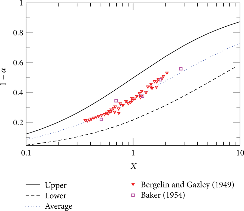
1-α versus X for different sets of data.
4. Summary and Conclusions
Simple expressions are developed for obtaining bounds for two-phase frictional pressure gradient and void fraction in circular pipes. The bounds approach is very useful in design and analysis, as engineers can then use the resulting average using the mean model and bounding values using the lower bound and the upper bound, respectively, in predictions of system performance. Also, the bounds approach is useful when conducting new experiments, since it provides a reasonable envelope for the data to fall within. The bounds are based on turbulent-turbulent flow assumption. Both the lower and upper bounds are based on the separate cylinders formulation. For frictional pressure gradient, the lower bound is based on the separate cylinders formulation that uses the Blasius equation to represent the Fanning friction factor while the upper bound is based on the separate cylinders equation that represents well the Lockhart-Martinelli correlation for turbulent-turbulent flow. For void fraction, the lower bound is based on the separate cylinders formulation that uses the Blasius equation to predict the Fanning friction factor while the upper bound is based on the Butterworth relationship that represents well the Lockhart-Martinelli correlation. These two bounds are reversed in the case of liquid fraction (1-α). The mean model is based on the arithmetic mean of lower bound and upper bound. For frictional pressure gradient, the model is verified using published experimental data of two-phase frictional pressure gradient versus mass flux at constant mass quality. The published data include different working fluids such as R-12, R-22 and Argon at different mass qualities, different pipe diameters, and different saturation temperatures. The bounds models are also presented in a dimensionless form as two-phase frictional multiplier (ϕ l and ϕ g ) versus Lockhart-Martinelli parameter (X) for different working fluids such as R-12, R-22, air-water and steam mixtures. For void fraction, the bounds models are verified using published experimental data of void fraction versus mass quality at constant mass flow rate. The published data include different working fluids such as steam, R-12, R-22, and R-410A at different pipe diameters, different pressures, and different mass flow rates. It is shown that the published data can be well bounded for a wide range of mass fluxes, mass qualities, pipe diameters, and saturation temperatures. The following conclusions can be drawn based upon the present study.
First, the present model is very successful in bounding the two-phase frictional pressure gradient and void fraction well for different working fluids over a wide range of mass fluxes, mass qualities, pipe diameters, and saturation temperatures.
Second, the present model is very successful in bounding two-phase frictional multiplier (ϕ l and ϕ g ), void fraction (α), and liquid void fraction (1-α) versus Lockhart-Martinelli parameter (X) well for different working fluids.
Third, the mean model provides a simple and acceptable means of predicting two-phase flow parameters.
Footnotes
Nomenclature
Conflict of Interests
The authors certify that they have no actual or potential conflict of interests including any financial, personal, or other relationships with other people or organizations within three years of beginning the submitted work that could inappropriately influence, or be perceived to influence, their work.
Acknowledgment
The authors acknowledge the financial support of the Natural Sciences and Engineering Research Council of Canada (NSERC) through the Discovery Grants Program.