Comparisons of Hydraulic Performance in Permanent Maglev Pump for Water-Jet Propulsion

Abstract

The operation of water-jet propulsion can generate nonuniform inflow that may be detrimental to the performance of the water-jets. To reduce disadvantages of the nonuniform inflow, a rim-driven water-jet propulsion was designed depending on the technology of passive magnetic levitation. Insufficient understanding of large performance deviations between the normal water-jets (shaft) and permanent maglev water-jets (shaftless) is a major problem in this paper. CFD was directly adopted in the feasibility and superiority of permanent maglev water-jets. Comparison and discussion of the hydraulic performance were carried out. The shaftless duct firstly has a drop in hydraulic losses (K₁), since it effectively avoids the formation and evolution of the instability secondary vortex by the normalized helicity analysis. Then, the shaftless intake duct improves the inflow field of the water-jet pump, with consequencing the drop in the backflow and blocking on the blade shroud. So that the shaftless water-jet pump delivers higher flow rate and head to the propulsion than the shaft. Eventually, not only can the shaftless model increase the thrust and efficiency, but it has the ability to extend the working range and broaden the high efficiency region as well.

1. Introduction

In many vessels, water-jets are required to achieve speeds of 30 + knots where conventional propeller solutions are unable to overcome the associated issues of cavitation, which in turn can lead to thrust breakdown and material failure. Any vessel designed for high speed requires a low resistance and corresponding slender hull [1]. However, this is not enough. The propulsor needs to be capable of accepting a high level of power. The function of the intake duct is to absorb the water from the hull bottom of the vessel and deliver it to the pump. The intake duct is also the major influence on the characteristic of the water-jet propulsion. Firstly, nearly 7%∼9% shaft power of the working propulsion is consumed in the duct [2]. Secondly, the interactions between the propulsion and the vessel which heavily affect the propulsion efficiency exist on the inlet of the duct. Finally, the flow losses in the intake duct also disturb the jet efficiency [3].

Many scientists have researched impact factors on the intake duct, such as the inclination, lip, ramp, IVR, and bend [4–6]. Bulten, 2006 [7], described the two-dimensional velocity field into the pump. Wei and Wang, 2009 [8], achieved the same description of the outflow field of the intake duct. Bulten [7] also used basic fluid dynamics theory to explain the development of nonuniform velocity contributed by the boundary layer ingestion, the deceleration of the flow, the bend, and the shaft. Hu and Zangeneh, 1999 [9], and Seil, 2001 [10], investigated the rotating shaft effect on the flow stability. But Hu and Seil selected intake duct as the research object instead of the propulsion which failed to consider the interaction between the pump and the intake, especially the effect of the rotating shaft on the performance of the water-jet propulsion.

In order to investigate the feasibility and superiority of the shaftless water-jet propulsion, this paper eliminated the upstream driving shaft and then used a passive magnetic pump by rim driven for water-jet system, where the rotor, stator, and intake duct are the major flow components.

Earnshaw in the year of 1893 theoretically proved that a magnetic body could not be supported in a stable manner in the field produced by any combination of mere passive magnetic poles [11]. That means it is impossible for a pure permanent maglev object to achieve stable equilibrium, because the force of attraction (or repulsion) between two magnetized bodies is inversely proportional to the square of their separation (distance). Precisely, there is no point of equilibrium between two magnets: they will attract or repel each other until they are attached together or separate indefinitely far away from each other. From energy viewpoint, the magnetic power in passive magnetic field has no minimal value point, at which any magnetic body needs energy increase to change its position. As a result, passive magnetic bearing has been disregarded for hundred years in spite of its many advantages, such as no friction and wear as compared to mechanical bearing, no need for complicated measurement and control as required by electromagnetic bearing, and no need for bulky cooling system that superconductive magnetic bearing has.

Earnshaw's theorem excluded the possibility of passive maglev because so few people conducted further research on passive maglev. But in the 21st century, Qian et al. [12] noted that Earnshaw's theorem was deduced in static status. In fact, Earnshaw's theorem is not applied in dynamic equilibrium of permanent maglev. There should be another theory to answer the question about whether a rotating passive magnetic levitator can achieve a stable equilibrium. Qian [13] introduced the gyroscopic effect to verify the feasibility.

High speed rotating object has a “Gyro-effect,” which enables the object to maintain the rotation stable. Gyro-effect can be understood as a function of inertia following Newton's First Law. This is as simple as riding a bicycle: with certain high speed, the rider can avoid falling, although theoretically a two-wheel bicycle cannot achieve stable equilibrium.

In Figure 1(a), there is a gyro stably rotating up a ball with high enough speed; but it will fall down the ball with lower speed. In Figure 1(b), a levitron [14] has the same property: the small ring can rotate contactlessly above the large ring when it rotates fast enough but will fall if its speed decreases to a certain value.

Figure 1:

Gyroscopic effect.

Things changed if the magnetic body moved. In 21st, Qian et al. [13, 15] proved that to achieve stable levitation, it is necessary to use a nonmagnetic force, and it is impossible to achieve stable levitation with passive magnetic forces alone. However, once stable levitation is achieved, it can be maintained using passive magnetic forces with other nonmagnetic forces, especially via the gyro-effect. A rotating magnetic object, for example, has not only passive magnetic energy but also dynamic energy. A patented novel passive magnetic bearing [15] was applied in rotary pump and turbine machine; Figure 2 shows that the rotors of these devices could be levitated in a stable manner if the rotating speed is high enough.

Figure 2:

Permanent maglev centrifugal pump and turbine.

This paper presents the prototype and model of permanent maglev pump for water-jet propulsion, demonstrates the stable levitation of the water-jet rotor, and discusses the hydraulic performance by theoretical analysis and numerical analysis.

2. Permanent Maglev Pump for Water-Jets

2.1. Original Research Object

The investigation focuses on the SDPM-450 water-jet propulsion. Its available ship speed (v_s) is 21∼42 knots. Its maximum power is 210 kw, and highest rotating speed is 2340 rpm. The design parameters of the corresponding water-jet pump include flow rate Q _d = 3200 m³/h, head H _d = 8 m, rotating speed n = 1750 rpm, and specific speed n _s = 976, where n_s is defined by (1). Table 1 lists the main geometric parameters of the water-jet pump, and the tested water-jet pump is shown in Figure 3. This pump is the fundamental object for the following improvement and optimization:

$n_s=\frac{\mathrm{3.65}n\sqrt{Q}}{H^{\mathrm{3}/\mathrm{4}}}=\mathrm{3.65}\left(\frac{\text{r}/\min ·{({\text{m}}^{\mathrm{3}}/\text{s})}^{\mathrm{1}/\mathrm{2}}}{{\text{m}}^{\mathrm{3}/\mathrm{4}}}\right).$

(1)

Table 1:

Main geometric parameters of water-jet pump.

Parameters	Values
Number of rotor blades z R	3
Rotor diameter D	450 mm
Hub diameter of rotor d hR	180 mm
Nozzle diameter D j	250 mm
Number of stator blades z S	7
Stator diameter D3	450 mm
Hub diameter of stator d hS	180 mm
Shaft diameter d	60 mm

Figure 3:

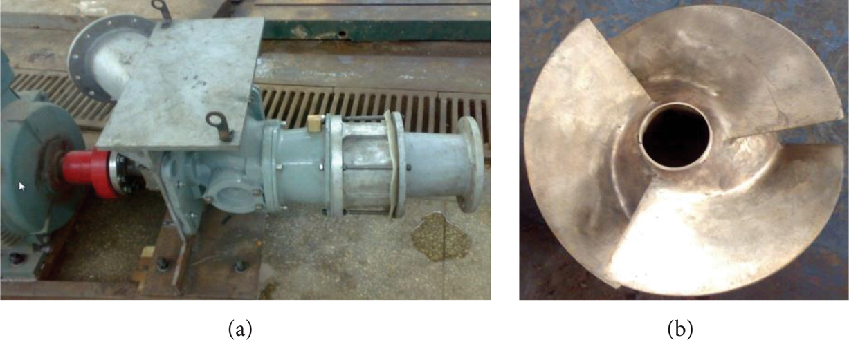
Tested pump and impeller.

2.2. Passive Magnetic Bearings

A patented novel passive magnetic bearing [15] is shown in Figure 4 (right), which has two passive magnetic rings with different outer and inner diameters but same thickness. The small ring is located beside the big ring concentrically and both are magnetized in the same axial direction. Compared with the available passive magnetic bearing (left) in Figure 4, which consists of two passive magnetic cylinders with the same length but different outer and inner diameters, the small cylinder is located within the big one. Both are magnetized in the same axial direction [16]. The novel bearing needs smaller axial occupation and has bigger axial magnetic bearing force and thus it is also used as an axial bearing except a radial bearing; the traditional passive magnetic bearing only has been used as a radial bearing [12].

Figure 4:

The available and novel permanent maglev rings.

2.3. Passive Magnetic Pump

According to the fundamental pump SDPM-450, the shaftless water-jet pump is the advanced model by using magnetic levitation technology. In Figure 5, shaftless water-jet pump was driven by the passive magnetic devices based on the former mechanism and bearings. First, the electrified motor coil produces rotational magnetic field. Then, the rotational magnetic field penetrates the distance sleeve and applies force on the rotor magnet and drives the rotor rotating. Assembled on both sides of distance sleeve, two couple novel passive magnetic bearings balance the radial and axial force. The magnetic force, fluid force, and gyro-effect together contribute to achieve stable dynamic equilibrium of permanent maglev. In Particular, the rotor of the water-jet pump is a passive magnetic levitator within the magnetic big rings and rotates stably with large enough speed. The critical speed between unstable to stable equilibrium may change according to the bearing force and the rotating inertia of the system: by larger bearing force or with larger inertia the critical speed will be lower [7]. Owning larger inertia, the axial flow rotor holds a lower critical speed than the centrifugal rotor. Based on the previous studies, the critical speed of the SDPM is less than 1300 rpm and nearly 75% of the design speed.

Figure 5:

Permanent maglev levitron of water-jets.

Disposed between the small and big magnetic rings, the isolation sets prevent fluid leakage as a sealing element and deliver the magnetic force as a transmission element. The isolation sets are closer to the big ring and motor, the unilateral radial gap is about 1.5 mm, and another gap between the rotor and isolation sets is nearly 2.5∼3.5 mm; the larger distance is satisfied with the eccentricity and vibration of the rotor under the operating condition. It is also beneficial to cool the magnetic devices. Under operating condition, the distance sleeve can bear high pressure and has little magnetic eddy current losses due to the high-strength plastic material. Above all, permanent maglev pump for water-jets has advantages of simpler structure, lower costs, and more reliability compared with other water-jet devices. The rim driven can improve the hydraulic performance by eliminating the shaft.

3. Numerical Simulation

CFD code ANSYS-CFX, which utilizes a finite-element based finite-volume method to discrete the transport equations, was used for numerical research. The fluid was split into four-component parts as shown in Figure 6. They were nozzle, stator, rotor, and simplified strait pipe with the shaft. This separation allowed each mesh to be generated individually and tailored to the flow requirements in that particular component. To get a relatively stable inlet and outlet flow, two times the rotor diameter had been extended in the inlet section.

Figure 6:

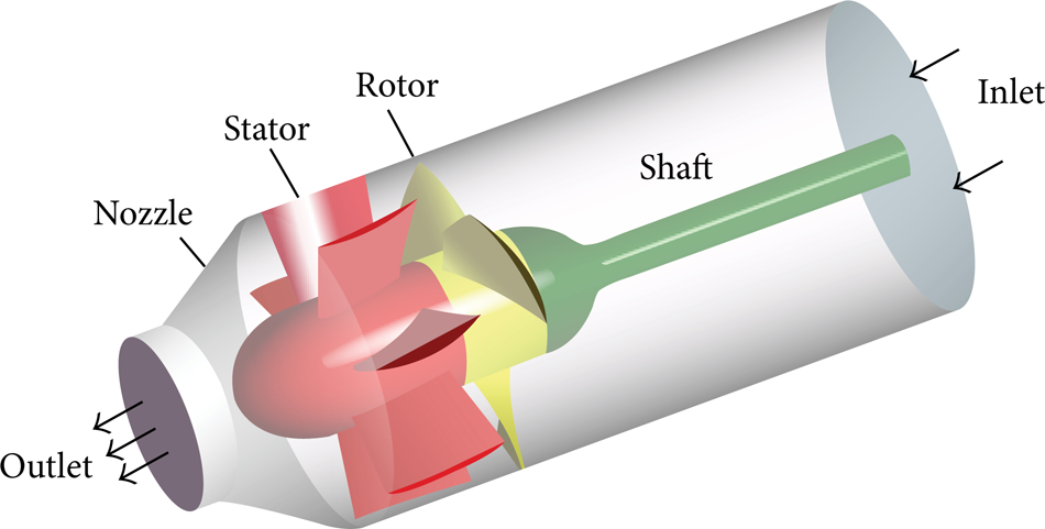
Water-jet pump.

3.1. Mesh Generation

ICEM-CFD was used to generate structured hexahedral grid for each component part. The tip mesh between the blades shroud and the rotor wall was paid attention to. Due to the complexity of generating structured mesh based on geometry, great efforts had been taken in the mesh generation of rotor and stator. The y + near the boundary wall was around 120. Figure 7 gives a view of the rotor and stator meshes.

Figure 7:

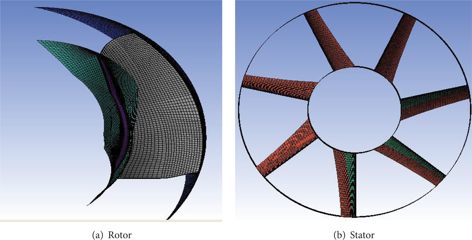
Mesh of rotor and stator.

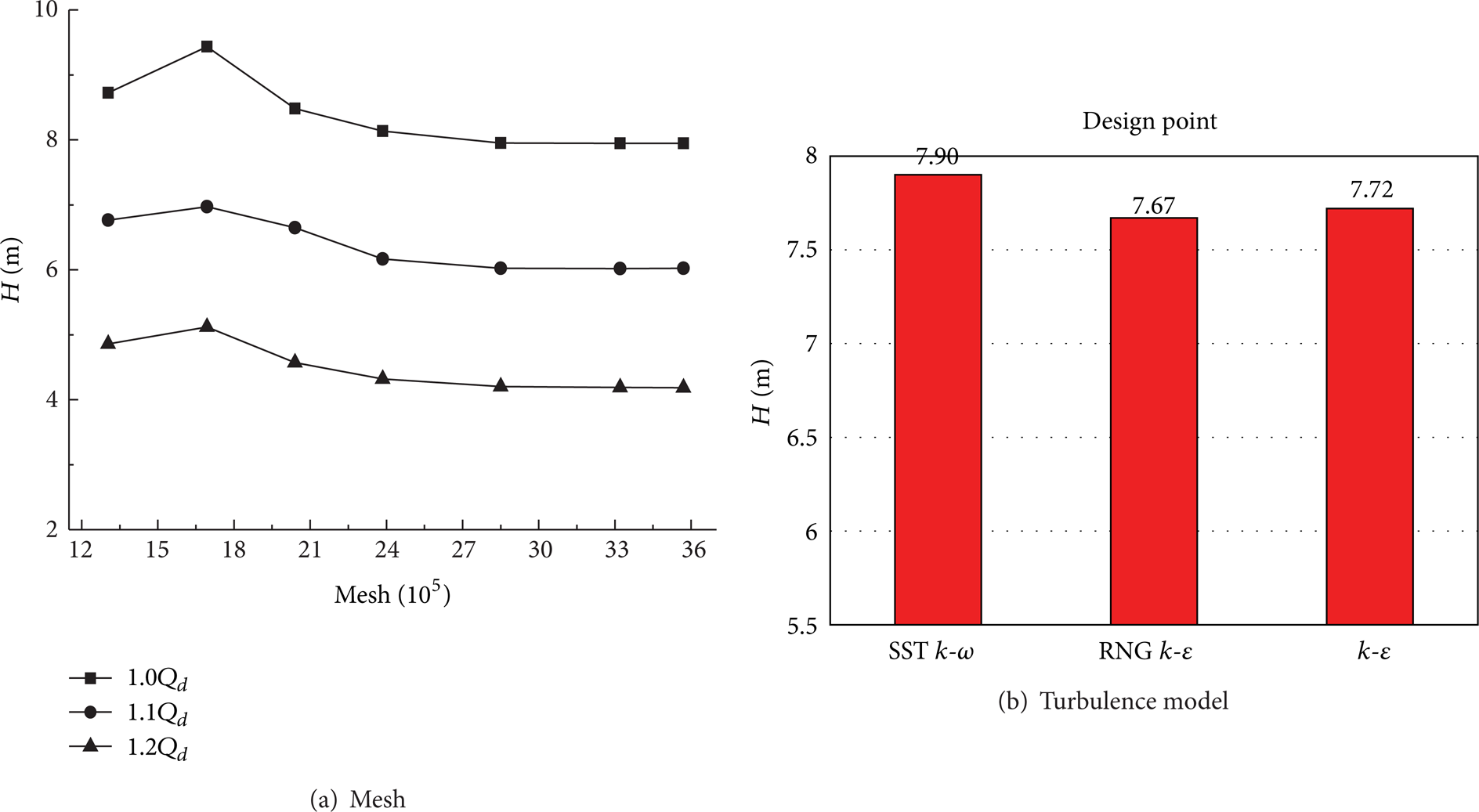
Ferziger and Peric pointed [17] out that more mesh contributes to higher precision of the simulation calculating. For this paper, ten models of mesh were constructed on domain to determine the mesh number, as shown in Figure 8(a). A grid independent test of three flow rates showed that when mesh numbers were around 2.76 million, the variation of head was within 1.0%. The final mesh numbers of nozzle, stator, rotor, and simplified strait pipe were 209710, 1088222, 1134956, and 329700, respectively. And the final mesh would be selected for the next analysis.

Figure 8:

Effect of mesh and turbulence model.

3.2. Boundary Details

In order to study the applicability of different turbulence models in the water-jet pump, turbulence models (standard k-ε, RNG k-ε, and SST k-ω) are selected to contrast applicability on the pump performance. It is observed that different turbulent models may have influence on the results in Figure 8(b), the error of 1.24% of SST k-ω is the lowest, RNG k-ε of 3.52% is second, and the highest is standard k-ε of 4.78% under designed condition. Therefore, the turbulence model SST k-ω holds the highest prediction accuracy of the performance.

Based on the former analysis, the SST k-ω model was selected. The advection scheme was set to high resolution. The convergence criterion was 10⁻⁵. The fluid selected was ideal water at 25°C. All the wall surface roughness within the control volume was set to 0.125 mm. The inlet and outlet boundary condition were set to static pressure inlet and mass flow rate outlet. After changing the mass flow rate, performance curves of the water-jet pump were acquired. As the motion of the rotor blades relative to the stationary stator was central to the investigation, the analysis must involve multiple frames of reference. The stator and nozzle were set in stationary frame and the rotor was set in rotary frame. The boundary wall of the shaft was set rotational at a speed of n = 1750 rpm. The interfaces between two stationary components, rotary, and stationary components were set to general grid and rotor stator interface, respectively.

3.3. Comparison of the Test and Simulation

A laboratory of a water-jet pump open test rig, as shown in Figure 9(a), was set up at Jiangsu University. Electric machine was used to drive the pump instead of the diesel engine, so the rotating speed must be decreased to 1450 rpm for the test. The inlet duct was a 45° elbow; a special flange connected the pump with the outlet pipe. To measure pump's torque and rotational speed, a torque meter was put between electric machine and water-jet pump. Its inlet and outlet pressure were measured by pressure gauges. After measuring pump's head, output power, and efficiency, performance curves were obtained, as shown in Figure 9(b). The uncertainty of measured pressure head (H), flow rate (Q), hydraulic power (P _h ), shaft power (P_shaft), and efficiency (η) were ± 0.14%, ± 0.50%, ± 0.52%, ± 1.08%, and ± 1.20%, respectively.

Figure 9:

Water-jet pump test bed.

Table 2 gives a comparison of simulated and tested results of the water-jet pump. It shows that the prediction data display greater than the tested head and pump efficiency; on the design condition the simulation model has the highest prediction accuracy, where the efficiency error is 0.46%, and the head error is 1.24%; on the off-design condition, the maximal head error is 8.29% and the maximal efficiency error is 6.08%. The explanation for maximal error on the 0.8 Q _d is that the backflow existed in the real flow of the pump. The explanation for major error on the 1.2 Q _d is that the simulation model did not consider the cavitation occurrence [5, 6]. Above all, the general mesh and the simulation model are able to predict the water-jet pump performance. It would be fundamental for the next analysis.

Table 2:

Comparison of tested and simulation data.

		0.8 Q d	0.9 Q d	1.0 Q d	1.1 Q d	1.2 Q d
Head	Test [m]	8.445	7.793	6.803	4.939	2.847
	Prediction [m]	9.146	8.137	6.888	5.112	3.035
	Error [%]	8.29	4.41	1.24	3.51	6.57
Pump efficiency	Test [m]	70.31	76.93	81.08	74.06	59.49
	Prediction [m]	74.59	79.79	80.71	75.99	61.75
	Error [%]	6.08	3.72	0.46	2.61	3.8

3.4. Simulation Model of Water-Jet Propulsion

Figure 10 shows the general flow of water-jet propulsion including a ship stern control volume which was regarded as the flow hull bottom of the ship. The ship stern control volume had the length of 30D, the height of 8D, and the width of 12D. It kept the same simulation model of water-jet pump, except the inlet and outlet boundary conditions. Both outflow boundary conditions were set to static pressure; the value was 1 atm.

Figure 10:

Numerical analyses on water-jet propulsion.

The velocity gradient of the bottom was considered in the inlet boundary condition; the thickness of boundary layer δ was calculated by Wieghardt equation.

The permanent maglev water-jets removed the driven shaft of SDPM-450 model; the theoretical and numerical analysis of the shaftless water-jet propulsion would be carried out in the next. The following comparisons and discussions of different water-jet propulsion (shaft and shaftless) were carried out by this simulation model.

4. Comparison and Discussion

4.1. Theoretical Analysis

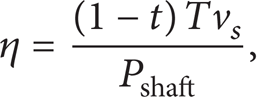
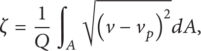
As evident from Figure 11, the water-jet pump is the working part of the water-jet propulsion. Meanwhile, the pump performances (head, pump efficiency, and flow) are relative to the water-jet propulsion characteristics (thrust and propulsion efficiency). Bulten [7] defined four equations (2)–(8) showing the relationships. Nonuniformity describes the uniformity of the flow field; ζ = 0 holds the best uniformity in (9). Another characterization is perpendicularity; θ = 90^° is the best one:

$T=\rho Q(v_j-\alpha v_s),$

(2)

Figure 11:

Flow field of water-jet propulsion.

There is a great relationship between the couple parameters and sailing conditions. The water that is ingested into the water-jet inlet channel partly originates from the hull's boundary layer. The mass averaged velocity of the ingested water (v_in) is lower than the ship speed due to this boundary layer. The velocity deficit is expressed as the momentum wake fraction (α). At the same time, the flow loss of the inlet duct is defined as the difference of total energy between capture area ahead of the intake (1) and the duct outlet (2). The degree of flow loss is usually described with loss coefficient K₁. It reflects the percentage of flow loss of the inlet duct to the kinetic energy of inflow upstream.

The propulsion efficiency (η) of different conditions is also restricted by the rotational speed (n) and ship speed (v_s). Simultaneous equations (2), (3), (4), and (5) solve the equal (12), the dimensionless expression of the propulsion efficiency. Jet velocity ratio (K) and wake fraction (α) are the major variable; rotational speed and ship speed indirectly impact the efficiency. According to the dimensionless expression of the propulsion efficiency, draw the η-K curves. Figure 12(a) is the efficiency curves with different wake fraction (α). Figure 12(b) is efficiency curves with loss coefficient of intake duct (K₁). The graph demonstrates that the propulsion efficiency curves offset to the greater value direction with the decreasing α and K₁. Videlicet the efficiency has inversely proportional function to α and K₁. As the performance parameters of intake duct, the variations of wake fraction and loss coefficient are difficult to inform by the theoretical methods, so flow field analysis would be applied.

Figure 12:

Curves of the efficiency.

4.2. Flow Field Analyses

4.2.1. Wake Fraction and Intake Duct Loss Coefficient

Calculation of the wake fraction and loss coefficient is rather complex, since the capture area is not known a priori. Determination of capture area can be done based on a well-defined control volume (streamtube). This can be set equal to the complete numerical domain, or it can be restricted to the cells. The fluid cells, which contain ingested water, are marked with a separate scalar. This scalar acts as a weight function after processing: 1.0 for ingested water and 0.0 for the other fluid. The streamtube can be visualised easily during this process with an isosurface plot. In such plot a surface is created, based on all cells with a constant value; in this case a concentration factor of 50% is used [18]. Figure 13 shows the water-jet installation and a plot of the streamtube. The shape of the streamtube has a semielliptical shape at the start of the numerical domain, and the capture area is positioned slightly forward of the inlet duct's ramp tangency point with a distance about one diameter of the duct outlet [19]. Based on the capture area, the wake fraction and loss coefficient can be calculated by equations.

Figure 13:

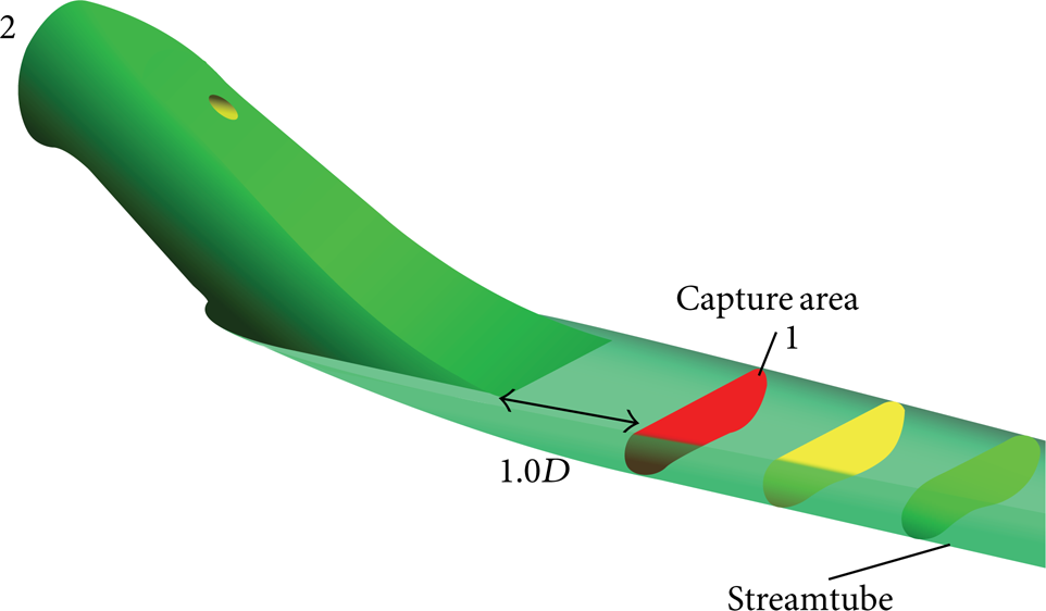
Streamtube and capture area.

To verify the former theoretical analysis, the numerical comparisons of the intake duct are shown in Figure 14. Wake fraction is actually on a linear function of the jet velocity ratio and the wake fraction has an increment with the increasing K, but the loss coefficient presents opposite variation trend. The shaft curves are nearly above the shaftless, so the shaftless intake duct possesses smaller α and K₁. Because of the inversely proportional function, the shaftless propulsion could obtain higher propulsion efficiency than the shaft one at the same K. Hence the shaftless model could improve the hydrodynamic performance of the duct and propulsion with smaller K₁ and α.

Figure 14:

Comparing the intake ducts.

4.2.2. Vortex and Helicity

The normalized helicity H _n has two further advantages to investigate the nature of vortex: first the swirl direction of a vortex is determined by the sign of helicity, so it is possible to differentiate between counter-rotating vortices. The second important point is that graduation in color for magnitude can clearly distinguish primary and secondary vortices. To locate and identify coherent structures the normalized helicity is used

$H=\left(1+K_j\right)\frac{v_j^2}{2g}+\left(\beta -K_1\right)\frac{v_s^2}{2g}+\Delta z,$

(3)

${\eta }_p=\frac{\rho gQH}{P_{\text{shaft}}},$

(4)

${\eta }_{}=\frac{(\mathrm{1}-t)T{v}_s}{P_{\text{shaft}}},$

(5)

$K=\frac{v_j}{v_s},$

(6)

$\alpha =\frac{v_{\text{in}}}{v_s},$

(7)

$\text{IVR}=\frac{v_p}{v_s},$

(8)

$\zeta =\frac{\mathrm{1}}{Q}{{\displaystyle \int }}_A^{}\sqrt{{\left(v-v_p\right)}^{\mathrm{2}}}dA,$

(9)

$\theta =\mathrm{90}-\frac{\mathrm{1}}{Q}{{\displaystyle \int }}_A^{}{v}_x\arcsin \left(\frac{v_x}{v}\right)dA,$

(10)

$K_{\mathrm{1}}=\frac{E_{\mathrm{1}}-E_{\mathrm{2}}}{\rho Q{v}_s^2/\mathrm{2}},$

(11)

$\eta =\mathrm{2}(\mathrm{1}-t){\eta }_P\frac{K-\alpha }{K^{\mathrm{2}}-{\alpha }^{\mathrm{2}}+(K_{\mathrm{1}}+K^{\mathrm{2}}{K}_j+Kz)}.$

(12)

$H_n=\frac{v·\omega }{\left|v\right|\left|\omega \right|}.$

(13)

Here, v and ω denote vectors of the relative flow velocity and the absolute vorticity, respectively. The normalized helicity is equivalent to the cosine of the angle between the absolute vorticity and the relative flow velocity. Therefore, if the value of formula (13) approaches ± 1 in the computational region, it shows that the core of longitudinal vortex exists on that region. The helicity H _n can be also interpreted as a rate characterizing the stability of a vortex. Value 1 indicates the maximum vortex stability including the momentum direction and the projection of spin, while −1 stands for the maximum instability of the vortex.

Further numerical analyses, improvements of the hydrodynamic performance, and evolutions of the vortex are carried out by normalized helicity. Observation planes in the intake duct are designated in Figure 15. On the design condition, the normalized helicity comparison between the shaft and shaftless duct is reflected in Figure 16.

Figure 15:

Observation profiles of the intake duct.

Figure 16:

Comparing the normalized helicity on design condition. (First and third columns are shaft; others are shaftless).

At the top of plane IX, there is a navy blue area (H _n = −1) in the shaft duct; it means that shaft duct generates an instable secondary vortex; at the same area in shaftless duct, there is a counter-rotating vortex generating; the normalized helicity is nearly 0.5. From plane IX to VII, both vortexes decay and break down; the secondary vortex of shaft duct has split to a pair of reserve vortex in plane VII, but shaftless duct delay to plane VI. The delaying vortex pair avoids interference from the shaft, rapidly dissipates in plane V, and is not able to impact the downstream. Compared with shaftless duct, the instable vortex pair of shaft duct split to some small vortex pairs around the shaft, and then vortex pairs are gradually shedding, dissipating, and consuming energy from plane VI to IV. As a result of the bend (planes IV to I), a new stable vortex is generated at the top of both ducts; this new vortex along the downstream evolves into a new vortex pair. The rotating shaft and the former vortex pairs of shaft duct result in bigger area of the stable vortex (H _n = 1) than the shaftless at the outlet.

Based on comparisons of the vortex evolution, the shaftless duct is able to generate the stable secondary vortex instead of the instable one then avert the interactions between the shaft and the vortex. So there are little vortex pairs generating, shedding, dissipating in the shaft reign of the shaftless duct; it could explain for the decrement of loss coefficient in the intake duct. Furthermore, the littler vortex pairs have less effect on the downstream of the shaftless duct; it can reduce the stable vortex into the pump and improves the nonuniform outflow field.

4.2.3. Nonuniform Outflow Field

The shaftless intake duct reduces the hydraulic losses and improves the flow field, so the next analysis would investigate on the outflow field of intake duct at the design rotating speed. Figure 17 shows the results. The nonuniformity of shaftless intake duct is less than the original one; the average decrement is 0.05. The decline curve is beneficial to improve the velocity outflow field.

Figure 17:

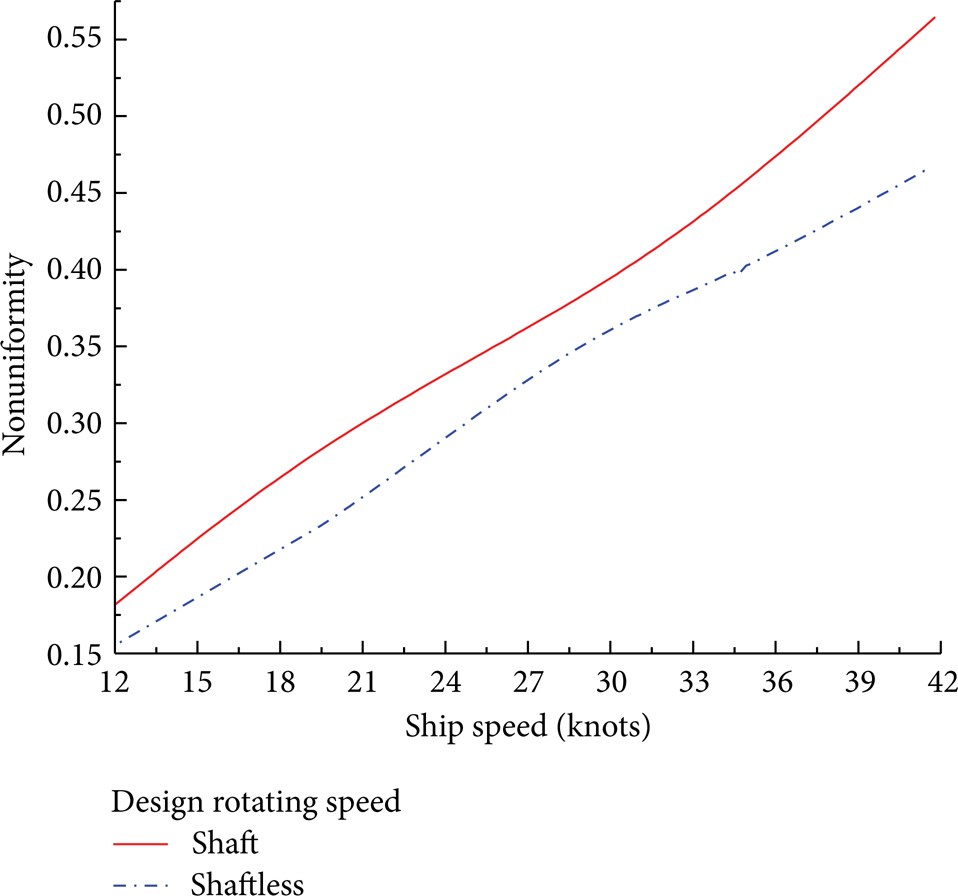
Nonuniformity comparison.

Actually, nonuniformity is an integrated variable to describe characteristics of the velocity; hence shaftless duct also improves the velocity field at the outlet. Figure 18 describes comparisons of circumferential and radial velocity components on the hub or shroud between the shaft and shaftless duct. The circumferential velocity (v_u) at 0.25r presents a sinusoidal distribution in Figure 18(a), the amplitude of shaftless duct is nearly half of the shaft, and the decrement of v_u at 0.75r is not obvious. In Figure 18(b), the radial velocity component (v_r) at 0.25r presents a cosine distribution; the removal of rotating shaft explains the 50% decrement of v_r. The shaftless also extends the period from 270° to 360° and drops the average line from 0.5 m to −0.2 m. At 0.75r, differences of v_r are unconspicuous. Both decreasing amplitudes verify improvements of the velocity field at the outlet, especially the region close to the shaft.

Figure 18:

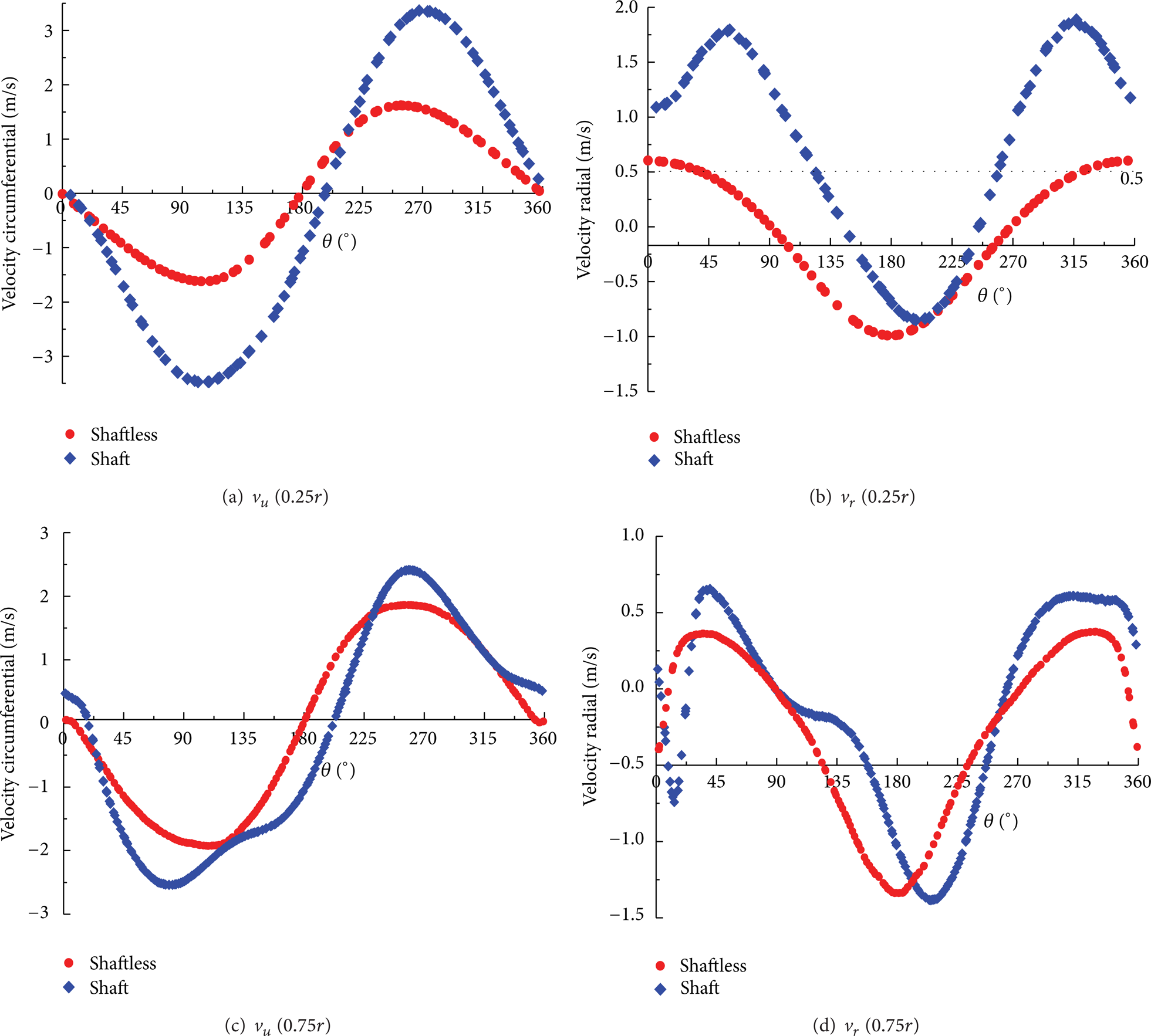
Comparison of velocity at the outlet on design condition.

Figure 18 also proves that the rotation shaft interferes with the velocity field of the intake duct. Removing the shaft is beneficial to make the distribution of velocity components close to trigonometric and decrease the amplitudes. As known to all, the outflow field of the intake duct is also the inflow field for the water-jet pump, so the shaftless water-jet pump could possess more uniform inlet flow field than the shaft one and reduce the effect of the inlet preswirl and radial velocity on the rotor, higher head and useful power may be delivered by the shaftless water-jet pump.

4.2.4. Velocity Inflow Field

To predict the performance of the shaftless water-jet pump, the velocity inflow field of the blade is focused on in the next research. A better uniform velocity field of the blade is shown in Figure 19 and compared with the original one on the design condition.

Figure 19:

Comparison of inflow velocity field of the rotor on design condition.

Results of comparison of the different preswirl were carried out, Figure 19(a). Shaftless water-jet pump benefits from less stable vortex and better velocity field at the outlet of shaftless duct. The inlet preswirl curve is below the shaft one, the average decrement is 0.8 m/s, and the decrement partially offsets the increment of nonuniform inflow to the shaft pump. The decreasing preswirl of the shaftless pump increases infinity flow angle β_∞; if airfoil placed angle β _L remains the same value, the airfoil attack angle Δα could directly increase too. Within a reasonable range, the increasing airfoil attack angle enhances the power capability of the shaftless water-jet pump; on the design condition the head may be higher than the shaft water-jet pump. At the same time, the decreasing preswirl of the shaftless pump also increases inlet flow angle β₁. Blade angle of the inlet keeps unchanged, so the flow attack angle Δβ₁ increases from negative to positive, and the increment of Δβ₁ can strengthen flow capacity of the shaftless water-jet pump. On the design condition, the flow rate may be higher than the shaft water-jet pump, so the shaftless water-jet pump holds better performance than the shaft.

Both meridional velocity distributions in Figure 19(b) indicate that v_m1 is not a constant. v_m1 varies invisibly from hub to r^* = 0.75 and drops rapidly from r^* = 0.75 to the shroud. It proves that, at the region close to the shroud, there is less fluid passes; in another way the backflow and blocking may exist at the shroud of the inlet. This phenomenon agrees with the real flow of the general stationary axial pump. But both velocity circulation distributions point out differences of flow characteristics between the water-jet pump and normal axial pump: Γ₁ is not equal to zero as the design assumption of the normal axial pump. Γ₁ has the opposite increasing tendency. The closer to the shroud, the greater the value of Γ₁; the inlet circulation must be considered in designing the axial water-jet pump.

Further comparisons, the improving uniformity of the water-jet pump inflow field optimizes the distribution of velocity circulation and meridional velocity at the inlet of rotor, as shown in Figures 19(b) and 19(c). At the region close to the shroud, Γ₁ of shaftless water-jet propulsion is lower than the original. The range of the stable Γ₁ extends from r^* = 0.7 (the radial location factor) to 0.8. It means that removing the shaft is beneficial to decrease the value of Γ₁ and reduce the backflow and blocking at the inlet shroud. Furthermore the change can improve the flow field at the inlet of the rotor and decrease the hydraulic losses of the water-jets, indirectly enhancing the work ability of the pump based on Euler's formula.

The inlet radial velocity curves are drawn in Figure 19(d). A huge difference exists between the shaft and shaftless pump, the shaftless curve approaches to the uniform inflow field. It indicates that shaftless model is able to compensate major effect of the nonuniform inflow on the distribution of v_r1. Although the v_r1 of the shaftless model is not ignored, applicability of the cylindrical layer independence assumption is enhanced, and the design method plays a better role in the design of water-jet shaftless pump.

Above all, the permanent maglev water-jet pump (shaftless pump) effectively improves the velocity inflow field of the blade and enhances the power and flow capacity of the pump. It infers that the shaftless water-jet pump has better performance than the original.

4.3. Performance Analyses

4.3.1. Head and Pump Efficiency

The couple parameters perpendicularity and nonuniformity of the inflow field analyzed effects of the shaft on characteristics of water-jet pump and results are shown in Table 3. Based on the nonuniform inflow, shaftless water-jet pump holds better uniformity than the shaft one under the same condition. There is also an increment of the head and pump efficiency; the maximum increment is about 1.75%. From another prospective, this table verifies the former surmise: the shaftless water-jet pump possesses a higher work capacity on the same flow. In other words the shaftless one has a stronger flow capacity on the same condition.

Table 3:

Comparison data of shaft and shaftless model.

Nonuniform	Shaft water-jet pump				Shaftless water-jet pump
Q [m3/s]	H [m]	η P [%]	ζ	θ	H [m]	η P [%]	ζ	θ
2570.57	9.992	69.633	0.1805	88.659	10.15	70.668	0.1744	88.665
2651.63	9.744	69.938	0.2221	88.688	9.901	71.258	0.2170	88.732
2732.64	9.253	69.490	0.2715	88.760	9.588	72.121	0.2643	88.816
2820.98	8.589	68.147	0.3244	88.782	9.122	72.493	0.3155	88.832
2982.79	7.423	64.019	0.3964	88.785	8.355	72.300	0.3861	88.837
3165.94	5.925	56.249	0.4572	88.789	7.503	71.372	0.4434	88.842

The former conclusion is that the shaftless water-jet pump can get higher performance at the same rotating speed, as shown in Figure 20. Based on (2), the head curve under the design ship speed is drawn; three curves have two points of intersection. Comparing the two points, the increments of head (ΔH) and flow rate (ΔQ) are displayed in the enlarged view and also enlarging with the increasing ship speed. With the unchanged nozzle diameter, more flow rate of the shaftless model obtains a higher jet velocity ratio than the original model. At the same ship speed, Figure 14 shows that the shaftless model decreases wake fraction so the assumption must be revised to the decrement of wake fraction. Based on thrust equation, shaftless water-jet propulsion future delivers more thrust.

Figure 20:

Theoretical schematic diagram.

At the same time, Figure 20(a) reveals that rotational speed and ship speed determine the operating point of water-jet pump. Formula (12) indicates that jet velocity ratio K holds corresponding function with the propulsion efficiency at the same rotational speed. Ship speed indirectly adjusts efficiency value interval by changing the range of the jet velocity ratio [20, 21]. In the same range of ship speed, the increment of K in shaftless water-jet propulsion results in the value interval of efficiency offsetting to larger jet velocity ratio direction. In order to remain the same value interval of efficiency, the ship speed of shaftless model has to increase Δv _s , as shown in Figure 20(b). It means that the complete efficiency curve has the tendency toward the higher speed direction t, especially the maximum point and the high efficiency area. So the ship would sail in the higher ship speed.

The shaft power is a constant value at the same rotating speed [22, 23]. Based on the propulsion efficiency equation, the shaftless model delivers more thrust and increases the propulsion efficiency on the same condition. Therefore, the complete propulsion efficiency curve also has the tendency towards up; the increment further broadens the work scope of shaftless water-jet propulsion. Above all, it is beneficial and available to remove the driven shaft in the intake duct with the theoretical analysis. The shaftless water-jet propulsion possesses higher thrust and efficiency than the original.

4.3.2. Thrust and Propulsion Efficiency

This chapter tidies numerical data of the shaft and shaftless water-jet propulsion. The data show that the shaftless one flows out more fluid than the original; the average increment is 60 m³/h at the design rotating speed. As the rotating speed decreases, the increment does not reduce straightly. The maximum average flow increment (100 m³/h) occurs at 0.83n. The increasing flow rate of water-jet propulsion verifies the former theoretical analysis. And comparisons of thrust and efficiency are shown in Figure 21.

Figure 21:

Analysis the performance of water-jet propulsion with and without shaft.

At the design point, the shaftless propulsion contributes to increase 3% thrust and 4% propulsion efficiency as shown in Figure 21. Figure 21(a) shows that the shaftless propulsion extends 3 knots working range with the design thrust and rotating speed, which could be explained by thrust equation and the increasing flow. At the design rotating speed, the thrust curve of the shaftless propulsion deviates from the design condition. In order to reach the design point, it is necessary to reduce the rotating speed. The decrease of rotating speed contributes to saving the shaft power and increasing the efficiency of the shaftless propulsion.

The maximum thrust increment is 20%, and the maximum range increment is 5 knots, as listed in Figure 21(a). The maximum propulsion efficiency increment is 15%, at the speed of 35 knots as listed in Figure 21(b). Referring to the former conclusion, because of the flow increment, the shaftless propulsion needs higher ship speed to get the same K. Therefore the ship speed range of the high propulsion efficiency skews towards right as presented in Figure 21(b). At the same time, the available working range and maximum efficiency point also present the same changing tendency. The maximum skewing value is 7 knots at the efficiency of 50%.

Above all, it verifies the theoretical conclusion of Section 4.3.1; the change (removing shaft) improves the performances: increasing the thrust and efficiency, broadening the working range, and extending the high propulsion efficiency range to the high speed.

5. Conclusion

The advanced model of SDPM-450 is a permanent maglev pump for water-jet propulsion and is also a passive magnetic levitator. The permanent maglev pump is driven by the passive magnetic devices instead of the rotating shaft. Based on the stable levitation mechanism and novel bearing, passive magnetic levitation of water-jet pump is achieved. The rotor can be maintained stable rotating by the balance between the passive magnetic forces, fluid force, and gyro-effect. Therefore, the permanent maglev pump simplifies the structure; there is no need for complicated measurement, control, and bulky cooling system. The permanent maglev pump also has better hydraulic performance and littler friction and wear than the original model.

The shaftless model minimizes the velocity nonuniformity and eliminates the flow separation around the shaft, so there are less energy losses in the intake duct. With the improvement of intake duct, it also reduces the backflow and blocking at the shroud of blade. More uniform inflow, less energy losses, and smaller wake fraction for the advanced duct are able to ensure better efficiency and reliability than the original duct.

Compared with the original pump, there is a greater increment of the performance for the permanent maglev water-jet pump, especially in the high ship speed region. Based on the theoretical formula, it infers that the increasing flow rate and head of the shaftless pump would deliver higher thrust to the vessel on the design condition (v _s = 30 knot), and the variation of jet velocity ratio would contribute to increasing and extending of propulsion efficiency.

Performance analysis shows that the permanent maglev model delivers more thrust (3%) than the traditional on the design speed. In order to match the resistance, the shaftless water-jet propulsion has to decrease the rotation speed of the engine to compensate for the increment of thrust. It means that the permanent maglev model could possess more efficiency (4%) and save more energy for operating. On the off-design condition, the shaftless model is proved to extend the working range and broaden the high efficiency region resulting from the increment of output volume.