Sage Journals: Discover world-class research

Abstract

The Internet of Things (IoT), which combines identification, sensing, computing, and communication technologies, is considered one of the major trends in information and communication technologies. Communication performance is critical for IoT applications. According to previous research, an internet-based overlay model is feasible for the implementation of the IoT. One important issue in the overlay routing model is the overlay node placement problem (ONPP). Once the size of overlay node set is fixed to a particular number k, the ONPP changes to k-ONPP. In this work, the IoT-based overlay node placement problem is formulized and analyzed. The major contributions of the paper include providing the time complexity of multi hop k-ONPP and its theoretical limit boundary of approximation ratio and proposing a local search algorithm. Furthermore, the time complexity and approximation ratio boundary of the local search algorithm are given. The proposed local search algorithm is evaluated by both time and efficiency where efficiency refers to the degree of approximation of algorithm results with optimal solutions. Another algorithm, TAG, is used for comparison. Finally, a simulation experiment based on network simulator EstiNet is provided. The experimental results show network delay benefits from the proposed method.

1. Introduction

The Internet of Things (IoT) has been regarded as the future of internet and one of the major trends in information and communication technologies [1]. The key idea of IoT is combining identification, sensing, computing, and communication technologies to provide a better description of physical processes. IoT technologies can be applied in a wide variety of applications such as smart homes, smart cities, environmental monitoring, and health care [2].

Many IoT-based applications require timely interaction between users and physical objects. Therefore, communication performance is very important in IoT implementation. There are three options for the implementation of the IoT: using the current internet, building a new network, and building a dual-layer network [3]. Based on the consideration of both performance and ease of implementation, an internet based dual-layer network is suitable for the IoT. Here, the dual-layer network refers to the overlay network. Currently, many IoT applications are implemented using an overlay network. Take the smart grid, for example. One typical example of a smart grid is the wide area management system (WAMS). The WAMS uses the phasor measurement unit (PMU) as sensor and data collector. The collected data need to be transferred to a control center for analysis. The current WAMS is built on an IP-based network, and many studies have been conducted on the influence of network performance on WAMS [4–6].

However, as the internet only provides a best-effort service, internet-based overlay networks should add additional methods to improve network performance. Such methods include admission control and overlay routing. Admission control guarantees the worst-case delay boundary, but it may deny a connection [7] and requires special network devices. Overlay routing has been proved useful in reducing end-to-end delay [8], and no further devices are needed. The overlay routing method can be used to reduce the communication delay between sensors and the data center where the data are analyzed. One important issue in the overlay routing model is the overlay node placement problem (ONPP) [9]. The objective of the ONPP is to find the optimal overlay node set with minimum total data transfer cost. However, the size of overlay node set may be fixed to a given number k due to cost and efficiency considerations. This modified ONPP is called k-ONPP.

In this work, the overlay node placement problem (ONPP) in IoT applications is formulized and a local search algorithm is proposed. The time complexity of k-ONPP is analyzed. Furthermore, we give the theoretical limit boundary of the approximation ratio for k-ONPP. Additionally, the approximation ratio boundary of the proposed local search algorithm is provided. A genetic algorithm and a greedy algorithm are introduced for performance comparison. All algorithms are evaluated by time cost and efficiency with MATLAB tools. Here, efficiency refers to the degree of approximation of algorithm results with optimal solutions. Finally, a simulation experiment based on the network simulator EstiNet [10] is provided to test the efficiency of the proposed overlay network model and algorithm. The experimental results show network delay benefits from the proposed method.

The rest of the paper is organized as follows. Section 2 introduces the research background and related work in overlay node placement. Section 3 presents the model and formulation of k-ONPP in the IoT and provides a theoretical analysis for this problem. Section 4 proposes a local search algorithm and provides its time complexity and approximation ratio boundary. Section 5 evaluates the algorithms based on time cost and algorithm approximation using MATLAB tools. A genetic algorithm and a greedy algorithm, TAG, are introduced for comparison. The local search algorithm is tested in a simulation scenario with the network simulator EstiNet in Section 6. Some additional factors that impact the algorithm are discussed. Finally, a general conclusion is provided in Section 7.

2. Research Background and Related Work

Overlay routing has been proved to be a feasible method to improve network performance with unreliable internet infrastructure [8]. The basic concept of overlay routing is choosing one or more nodes in the overlay network as hop nodes for data transfer. Overlay routing will use an additional routing algorithm, separate from the underlying internet routing algorithm. There are two types of overlay networks: peer-to-peer networks and infrastructure networks [9]. Network nodes of peer-to-peer networks may change rapidly, while the nodes of infrastructure networks have higher persistence. In most infrastructure overlay networks, overlay nodes belong to a single entity, so it is feasible to apply the routing algorithm in these overlay nodes. Currently, most networks of IoT applications are similar to infrastructure overlay networks, so this paper focuses on the overlay node placement problem in such networks.

Previous work in [8] has proved that with the overlay routing method, the RTT of end-to-end packet may be reduced. Andersen et al. found that network performance would improve with only one hop node [11]. A random-k algorithm is proposed in [12]. The basic idea of this algorithm is randomly selecting k nodes out of M. Then, a source sends a test packet through these k nodes to the destination. The intermediate node whose response comes back first will be chosen as the overlay node. This algorithm aims to improve the network reliability after path failure occurs, so other performance metrics such as communication delay are not considered. Additionally, this algorithm is based on experimental experience, no theoretical analysis is given.

In [13], Zhu et al. further studied the node placement problem with one hop node. Their scenario uses overlay routing and multihoming to improve network performance and availability. They proved the overlay node placement problem with one hop node which is an NP-hard problem based on a reduction from the set covering problem. The number of overlay nodes is not fixed in their scenario. In contrast to previous work in [12], network performance is considered in [13]. Four heuristic methods, Random, Customer-driven, Traffic-driven, and Performance-driven, are introduced and tested. Their results show an improved RTT from sources to destinations with overlay routing.

A measurement study on the benefits from overlay routing is made in [14]. Their scenario uses overlay routing to improve end-to-end network performance. The intermediate node is also set to be one. In contrast to previous work in [11–13], the number of overlay nodes is fixed to a given number k in this work. The problem is also proved to be an NP-hard one. Four greedy heuristic algorithms are introduced and tested.

A generic description of k-ONPP is given in [9] as follows. Given M possible overlay nodes and a number k, choose k nodes out of M to optimize the application-specialized performance metric. Moreover, the number of intermediate nodes in an overlay path is unfixed. In [15], Yang et al. considered this generalized problem with the performance metric group delays from sources to destinations. In this work, the node placement problem is described by a linear programming formula and solved with ILOG CPLEX, an optimization software package designed by IBM. Although in this work the generalized problem is considered, it is unfeasible to implement the solution in a real network as the results are calculated by another software.

The latest work on overlay node placement problem can be found in [16–18]. In [16], Roy et al. introduced a greedy algorithm called Traffic Aware Greedy (TAG) and compared this algorithm with the node degree-based algorithm. Another greedy algorithm is proposed in [17]. Cohen and Raz made progress on this problem by providing a theoretical limit boundary of the approximation ratio that can be achieved by a polynomial algorithm based on the set cover problem [18]. The overlay node placement problem also has been discussed in other contexts such as web cache placement in [19, 20], but the motivation and objective are quite different.

As described above, most of the current works on the overlay node placement algorithm are greedy algorithms and lack a theoretical analysis. Although [18] analyzed this problem in a theoretical manner and provided a limit boundary of approximation ratio, their analysis is based on a one-hop overlay. In addition, the approximation ratio of their proposed algorithm is denoted by another parameter m, where m is the size of the maximum minimal overlay vertex cut. As written in [18], finding the minimal overlay vertex cut is not easy. In this work, the overlay node placement model for IoT applications is proposed, and a different analysis approach is made based on a reduction from the k-median problem. We further analysis the k-ONPP problem with a multihop overlay and provide its time complexity and the limit boundary of the approximation ratio. A local search algorithm is proposed, and the approximation ratio boundary has been provided in a more calculable way.

3. Problem Formulation and Analysis

According to previous research in IoT [21, 22], the architectural of IoT can be divided into three parts: sensor/actuator layer; information transmission layer (network layer), and application layer. As mentioned in the introduction, currently the internet based dual-layer network is feasible for an IoT application, so an abstract IoT architectural scheme can be described as in Figure 1.

Figure 1

IoT architectural scheme.

Consider the above IoT architectural scheme, the communication network of IoT is used for data gathering from distributed sensors to analysis centers. Some data concentrators, such as PMU in smart grid, are deployed so that an internet-based dual layer network is already there. These concentrators and sensors are fully constructed and controlled by the same entity or group, so they can be used as an overlay node to gain benefits. As these concentrators are almost persistent, this overlay network can be regarded as an infrastructure overlay network. Thus, the problem is how to place these concentrators to maximize the benefits. Figure 2 in the following page provides a sketch map of such a dual layer network.

Figure 2

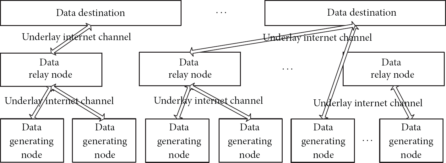
Sketch map of a dual layer network of the IoT.

3.1. Problem Formulation

We consider the performance metric of group communication delay, which is the total communication delay from each sensor to the analysis center. Group communication delay is used because data generated by sensors in IoT application is predictable and generally periodic. This means that if group communication delay drops, system performance may become better. Then, the overlay node placement problem can be formulized as follows.

Consider a physical network represented as a graph $G (V, E)$ , where V denotes the networking devices and E denotes links between V. The weight of link e in E is defined by a metric such as network bandwidth or communication delay, denoted by $l_{i j} > 0$ , where $i, j$ indicates the vertexes of link e. We use communication delay as metric. A group of source vertexes denoted by S needs to send data to destination vertexes denoted by T. A candidate set of vertexes $B \subseteq V$ may be suitable locations to deploy concentrators. Let $O \subseteq B$ denote the chosen overlay node set. The destination of each $s \in S$ is fixed to $t \in T$ . We define the function $t (s)$ , which denotes the t that s is connected to. Once the overlay node set O is chosen, each of the source vertexes $s \subseteq S$ can use O to transfer data. Let $l_{p}^{s, t (s)}$ indicate the weight of the direct path from vertex s to $t (s)$ and $l_{O}^{s, t (s)}$ indicate the weight with overlay nodes. $l_{O}^{s, t (s)}$ is the weight of shortest path with overlay set O. Suppose that the shortest overlay path from s to $t (s)$ is $(s, o_{1}, o_{2}, \dots, o_{k}, t (s))$ then $l_{O}^{s, t (s)} = l_{s o_{1}} + l_{o_{1} o_{2}} + \dots + l_{o_{k} t (s)}$ . If overlay set O is not helpful to reduce the original weight, then s will link directly to $t (s)$ . Then, $l_{O}^{s, t (s)} = l_{p}^{s, t (s)}$ . We define $l_{p}^{t (s), t (s)} = l_{O}^{t (s), t (s)} = 0$ ; then, $l_{O}^{s, t (s)}$ can be defined as follows:

l_{O}^{s, t (s)} = min_{o \in {O + {t (s)}}} (l_{p}^{s, o} + l_{O}^{o, t (s)}) .

(*)

Clearly,

l_{O}^{s, t (s)} \leq l_{p}^{s, t (s)}

. This is different from other discussions, as in others each source must connect to one overlay node. Then, the objective function can be written as finding

O \subseteq B

to minimize

\sum_{s \in S} l_{O}^{s, t (s)}

, where

t (s)

is defined above and denotes the destination

t \in T

to which s connects. Considering the cost of deploying these overlay nodes and the cost of maintaining communication delay information between the overlay nodes, the size of set O should be limited. Suppose that a given number k is used. We define this problem as the k-ONPP problem. Then, the problem is modified to finding

O \subseteq B

to minimize

\sum_{s \in S} l_{O}^{s, t (s)}

, and the size of O is k.

3.2. Problem Analysis

In this section, we will analysis the time complexity for k-ONPP and discuss the theoretical limit boundary of approximation ratio. We give the following theorems.

Theorem 1.

k-ONPP is an NP-hard problem.

Proof.

First, we consider another NP-complete problem. The k-median decision problem is a typical NP-complete problem which can be described as follows. Given a client set $\hat{C}$ and a candidate position set $\hat{B}$ , the weight from each $\hat{c} \in \hat{C}$ to $\hat{b} \in \hat{B}$ is denoted by ${\hat{l}}_{\hat{c} \hat{b}} > 0$ . Determine whether there exists a set $\hat{O}$ out of $\hat{B}$ where the size of $\hat{O}$ is k such that

\begin{matrix} \sum_{\hat{c} \in \hat{C}, \hat{o} \in \hat{O}} \min ({\hat{l}}_{\hat{c} \hat{o}}) \leq U . \end{matrix}

(1)

We define this problem as

P_{1}

. Then, we consider a modified problem from k-ONPP as follows. Consider a graph

G (V, E)

, a source set S, a destination set T, and a possible set B. Find

O \subseteq B

to minimize

\sum_{s \in S, o \in O} \min (l_{p}^{s, t (s)}, l_{p}^{s, o} + l_{p}^{o, t (s)})

, where the size of O is k. Define this problem as

P_{2}

. This objective function means that at most only one overlay hop can be used in an overlay path. Consider the decision problem

P_{2}

, determining whether there exists a set O out of B where the size of O is k such that

\begin{matrix} \sum_{s \in S, o \in O} \min (l_{p}^{s, t (s)}, l_{p}^{s, o} + l_{p}^{o, t (s)}) \leq U . \end{matrix}

(2)

We define this problem as

P_{3}

Next, we modify problem $P_{3}$ into a different version. Let $\hat{B} = B$ , $\hat{C} = S$ , and $\hat{k} = k$ . Consider a client point $\hat{c} \in \hat{C}$ and a candidate overlay node $\hat{b} \in \hat{B}$ . Define

\begin{matrix} {\hat{l}}_{\hat{c}, \hat{b}} = \min (l_{p}^{s, t (s)}, l_{p}^{s, b} + l_{p}^{b, t (s)}) . \end{matrix}

(3)

Then, problem

P_{2}

changes to determining whether there exists a set

\hat{O}

out of

\hat{B}

where

Size (\hat{O}) = \hat{k}

such that

\sum_{\hat{c} \in \hat{C}, \hat{o} \in \hat{O}} \min ({\hat{l}}_{\hat{c} \hat{o}}) \leq U

. It is obvious that modified problem

P_{3}

is the same as problem

P_{1}

. Because

P_{1}

is NP-complete, then

P_{3}

is NP-complete as well. Additionally, this proves that problem

P_{2}

is the same as the k-median problem.

Now, we consider the original k-ONPP. Given a graph $G (V, E)$ , a source set S, a destination set T, and a possible set B, find $O \subseteq B$ to minimize $\sum_{s \in S} l_{O}^{s, t (s)}$ , where the size of O is k. Suppose there is a polynomial algorithm for k-ONPP. Construct a special case of k-ONPP. Let $l_{p}^{b_{1}, b_{2}} = T ≫ l_{p}^{s, t (s)}$ , where $b_{1}, b_{2} \in B$ and $s \in S$ . Obviously, in this constructed k-ONPP, only one hop node at most may be used in the overlay path. If there is a polynomial algorithm for k-ONPP, then the constructed k-ONPP can be solved, then problem $P_{3}$ can be solved. The algorithm for $P_{3}$ can be designed as follows. (1)

Use the polynomial algorithm for k-ONPP to find the result R of constructed k-ONPP.

(2)

Test if $R \leq U$ .

Because

P_{3} \propto k

-ONPP and

P_{3}

is NP-complete, k-ONPP is an NP-hard problem. This proves Theorem 1.

Next, we provide the theoretical limit boundary of an approximation ratio for k-ONPP. In k-ONPP, define following parameters:

\begin{array}{l} d_{\max} = \max {\min (l_{p}^{s, t (s)}, l_{p}^{s, b} + l_{p}^{b, t (s)}) \\ ∣ t (s) \in T, s \in S, b \in B}, \\ d_{\min} = \min {\min (l_{p}^{s, t (s)}, l_{p}^{s, b} + l_{p}^{b, t (s)}) \\ ∣ t (s) \in T, s \in S, b \in B}, \\ ω = \frac{d_{\max}}{d_{\min}}, \\ α = \max {\frac{l_{p}^{s, b} + l_{B}^{b, t (s)}}{l_{p}^{s, b} + l_{p}^{b, t (s)}} ∣ t (s) \in T, s \in S, b \in B} . \end{array}

(4)

Theorem 2.

There is no polynomial algorithm for k-ONPP with an approximation ratio less than $α \times (1 + ((ω - 1) / e))$ .

Proof.

As proved above, problem $P_{2}$ is the same as k-median problem. With the above-defined $d_{\max}$ and $d_{\min}$ , ω also denotes $\max {\hat{l}}_{\hat{c}, \hat{b}} / \min {\hat{l}}_{\hat{c}, \hat{b}}$ , where $\hat{b} \in \hat{B}$ in problem $P_{1}$ . Pan et al. proved that with a so-defined ω, there are no polynomial algorithms with an approximation ratio less than $1 + ((ω - 1) / e)$ unless $NP \subseteq DTIME (n^{O (\log \log n)})$ for a general distance space k-median problem [23]. Let the optimal result for $P_{2}$ be $O_{1}$ and the optimal result for k-ONPP be $O_{2}$ . Let the best result which can be obtained with polynomial algorithm for $P_{2}$ be $R_{1}$ and the best result which can be obtained with a polynomial algorithm for k-ONPP be $R_{2}$ . Obviously, we have $O_{2} \leq O_{1}$ , $R_{2} \leq R_{1}$ . Because $R_{1} / O_{1} \geq (1 + ((ω - 1) / e))$ , $R_{2} / O_{2} \geq R_{2} / O_{1} \geq R_{2} / R_{1} \times R_{1} / O_{1}$ . However, for each overlay path for client $s \in S$ , $\min (l_{p}^{s, t (s)}, l_{p}^{s, o} + l_{O}^{o, t (s)}) \geq \min (l_{p}^{s, t (s)}, l_{p}^{s, b} + l_{B}^{b, t (s)}) \geq α \times \min (l_{p}^{s, t (s)}, l_{p}^{s, b} + l_{p}^{b, t (s)})$ . Therefore, $R_{2} / R_{1} \geq α$ and $R_{2} / O_{2} \geq α \times (1 + ((ω - 1) / e))$ . This proves Theorem 2.

Both α and ω are easy to calculate in this formula. It is obvious that the time complexity to obtain ω is $O (Size (S) \times Size (B))$ . The time complexity to obtain α is the time complexity of shortest path algorithm. Because $l_{B}^{b, t (s)}$ means using whole candidate set B as overlay node set, the shortest path algorithm can be applied.

4. Proposed Algorithm and Analysis

As discussed above, the k-ONPP problem is similar to the k-median problem, so the algorithm for the k-median problem may also be applied in k-ONPP. The proposed local search algorithm is modified from the local search algorithm developed by Arya et al. in [24]. However, the discussion in [24] is based on the metric space, which means that the distance definition satisfies the symmetrical characteristic and triangle inequality. However, neither of these two properties is consistent with network delay. In fact, if network delay satisfies triangle inequality, there is no need to optimize the delay as $l_{p}^{s, t} \leq l_{p}^{s, a} + l_{p}^{a t}$ . The modified local search algorithm works as follows.

We define the cost function as Cost $(N)$ with given set N, which indicates the group communication delay from the client set S to destination T with a given overlay set N. A neighborhood structure for the set N is defined as $F (N) = {N - n + m ∣ n \in N, m \in B, m \notin N}$ . We define a local optimum as $Cost (N) < Cost (N^{'})$ for all $N^{'} \in F (N)$ . Then, the steps of proposed local search algorithm are described in Algorithm 1.

Algorithm 1: Proposed local search algorithm.

Algorithm: Local Search Algorithm

Input: Candidate set B; Cost function $C o s t (N)$ ; Neighborhood structure $F (N)$ ;

Delay graph $G (V, E)$

Output: Sub-optimal overlay node set O

(1) Random select a set N which $S i z e (N) = k$

(2) Constructing a new graph $G^{'} (V^{'}, E^{'})$ with $V^{'} = {N, {t (s)}}$

(3) Apply Dijkstra algorithm in $G^{'}$ to get the shortest path from N to ${t (s)}$

(4) Calculating the $C o s t (N) = \sum_{s \in S} \min_{n \in N} (l_{p}^{s, n} + l_{N}^{n, t (s)})$

(5) If $\exists N^{'}$ $\in F (N)$ that $C o s t (N^{'}) < C o s t (N)$ then $N = N^{'}$ , return to Step 1

(6) Return N.

Next, we discuss the time complexity of the proposed algorithm. We state the following theorem.

Theorem 3.

The time complexity of the proposed local search algorithm is polynomial.

Proof.

Let $Size (B) = M$ , where p indicates the number of iterations. Suppose that $k ≪ N$ . The time cost for the Dijkstra algorithm is $O (k^{2})$ . The maximum replacement in each iteration for set N is $Size (B - N)$ . So, the total time complexity for local search algorithm is $O (k^{2} M p)$ . As discussed in [24], p can be defined as $p = \log (Cost (S_{0}) / Cost (O)) / \log (1 / (1 - ε / Q))$ . Here, $S_{0}$ is the initial value, O is the optimal result, $ε > 0$ is constant, and Q is the size of $Θ \subset G (S)$ , where S is the set of all feasible solutions and $G (S)$ is the neighborhood of S. With proposed local search algorithm $G (S) = F (S) = {S - n + m ∣ n \in S, m \in B, m \notin S}$ ; therefore, $Q \leq Size (S) \times Size (B - S)$ , which is polynomial because Q, $\log (Cost (S_{0}))$ and $\log (Cost (O))$ are polynomial with the input size. So, the time complexity of the local search algorithm is polynomial. This proves Theorem 3.

Finally, we provided the approximation ratio boundary of the local search algorithm in Theorem 4.

Theorem 4.

The approximation ratio boundary of the proposed local search algorithm is $ω / α$ .

Proof.

Suppose that the optimal set for k-ONPP is O and local optimal set is N. Let $O = (o_{1}, o_{2}, \dots, o_{k})$ and $N = (n_{1}, n_{2}, \dots, n_{k})$ . $d_{\max}$ and $d_{\min}$ are defined the same as before, $ω = d_{\max} / d_{\min}$ . As N is the local optimal set, then for all $N^{'} \in F (N)$ , we obtain

\begin{matrix} Cost (N^{'}) - Cost (N) > 0 . \end{matrix}

(5)

From inequality (5), we replace the overlay node

n_{1}

in N with node

o_{1}

in O, then we obtain

\begin{matrix} Cost (N - n_{1} + o_{1}) - Cost (N) > 0 . \end{matrix}

(6)

Define

N_{1} = (o_{1}, n_{2}, \dots, n_{k})

N_{2} = (n_{1}, o_{2}, \dots, n_{k}), \dots

N_{k} = (n_{1}, n_{2}, \dots, o_{k})

. Define

D_{C} (o_{1})

as the clients which connect

o_{1}

as first overlay node. For

N_{1}

, let

c \in D_{C} (o_{1})

connect to

o_{1}

as first overlay node, and let

c^{'} \in C - D_{C} (o_{1})

connect to

n^{'} \in {N_{1} + {t (c^{'})}}

with minimum min

(l_{p}^{c^{'}, n^{'}} + l_{N_{1}}^{n^{'}, t (c^{'})})

. Therefore, inequality (6) can be expanded as follows:

\begin{array}{l} Cost (N - n_{1} + o_{1}) - Cost (N) \\ = \sum_{c \in D_{C} (o_{1})} (l_{p}^{c, o_{1}} + l_{N_{1}}^{o_{1}, t (c)} - l_{N}^{c, t (c)}) + \sum_{c \in C - D_{C} (o_{1})} (l_{N_{1}}^{c, t (c)} - l_{N}^{c, t (c)}) \\ > 0 . \end{array}

(7)

For the first portion before the plus sign in (7),

\begin{array}{l} d_{\min} \leq \frac{1}{α} \min (l_{p}^{s, t (s)}, l_{p}^{s, b} + l_{B}^{b, t (s)}) \\ \leq \frac{1}{α} \min (l_{p}^{c, t (c)}, l_{p}^{c, o} + l_{O}^{o, t (c)}) = \frac{1}{α} l_{O}^{c, t (c)} \\ l_{p}^{c, o_{1}} + l_{N_{1}}^{o_{1}, t (c)} \leq l_{p}^{c, o_{1}} + l_{p}^{o_{1}, t (c)} \leq ω d_{\min} \leq \frac{ω}{α} l_{O}^{c, t (c)} . \end{array}

(8)

For the second portion in (7),

\begin{matrix} l_{N_{1}}^{c, t (c)} \leq l_{p}^{c, t (c)} \leq ω d_{\min} \leq \frac{ω}{α} l_{O}^{c, t (c)} . \end{matrix}

(9)

So, inequality (7) can be expanded as follows:

\begin{array}{l} 0 < \sum_{c \in D_{C} (o_{1})} (l_{p}^{c, o_{1}} + l_{N_{1}}^{o_{1}, t (c)} - l_{N}^{c, t (c)}) + \sum_{c \in C - D_{C} (o_{1})} (l_{N_{1}}^{c, t (c)} - l_{N}^{c, t (c)}) \\ \leq \sum_{c \in D_{C} (o_{1})} (\frac{ω}{α} l_{O}^{c, t (c)} - l_{N}^{c, t (c)}) + \sum_{c \in C - D_{C} (o_{1})} (\frac{ω}{α} l_{O}^{c, t (c)} - l_{N}^{c, t (c)}) \\ = \sum_{c \in C} (\frac{ω}{α} l_{O}^{c, t (c)} - l_{N}^{c, t (c)}) = \frac{ω}{α} Cost (O) - Cost (S) . \end{array}

(10)

Then, we have obtained the approximation ratio with defined ω and α as follows:

Cost (S) < \frac{ω}{α} Cost (O) .

(**)

This proves Theorem 4.

5. Algorithm Evaluation

In this paper, the proposed local search algorithm is tested with both Matlab and the network simulator EstiNet. EstiNet is used to test the algorithm's performance in a network environment. However, as the amount of network nodes is limited in a simulator, in this section, Matlab is used to evaluate the algorithm based on time cost and effectiveness. A genetic algorithm is introduced to approach the optimal result, while the TAG algorithm proposed in [16] is used for comparison.

5.1. Experiment Design and Implementation

As described above, a physical network can be represented as a graph $G (V, E)$ , where V denotes networking devices and E denotes the time delay between V. In the actual network, networking devices are connected in two modes: directly connecting with links and indirectly connecting with routers or switchers. So, the first step of experiment is generating an $M \times M$ matrix to record the graph, where M is the number of network devices. After that, direct connections with time delay between graph vertexes are randomly generated. In the third step, each pair of two vertexes in the graph is connected through the directly connecting vertexes. The time delay between indirectly connecting vertexes is the sum of the time delay between directly connecting vertexes in the path.

The Matlab test is implemented on a laptop with two Intel i5 core processors and 3 GB memory. For each experiment, we test the algorithm 500 times. The mean value of the proposed algorithm is then calculated to better expose the performance. In addition, the 95% quartile of 500 tests is calculated and the 95% confidence interval of the mean value is obtained. For the genetic algorithm, the best result of the 500 tests will be recorded, as it is used to generate the optimal result.

5.2. Two Other Algorithms for Comparison

5.2.1. Genetic Algorithm

To evaluate the time cost and algorithm approximation, the global optimal result is needed for comparison. However, as previously proved, k-ONPP is NP-hard; we cannot calculate the global optimal solution with an increasing problem scale. So, the result of a genetic algorithm is used to approximate the global optimal result. It is unnecessary to provide the detailed steps of the genetic algorithm, so only the key definitions are described here as follows. (1)

Genetic representation. The target of k-ONPP is finding k nodes out of possible set B to minimize group delay. A natural thought is using the tag of these nodes to represent the solution. So, we mark each node in set B with a number and represent each individual as a set of numbers. The size of the individual set is fixed to k.

(2)

Fitness function. The property of the fitness function is that the better the solution is, the larger the fitness will be. However, the cost function defined above is the group delay. Suppose that N denotes current generations and C denotes the fitness of calculated individual. We define fitness function as follows:

\begin{matrix} 1 - \frac{Cost (C) - \min (Cost (N))}{\max (Cost (N)) - \min (Cost (N))} . \end{matrix}

(11)

(3)

Crossover. Randomly choose the crossover point in an individual set. Then, the tag number before or after the crossover point is swapped. However, the same point may appear twice in a single individual set after crossover. For example, this occurs if individual A is (3, 4, 7, 9); individual B is (1, 3, 5, 7), and the crossover has happened at the second point; one of the results is (3, 3, 5, 7). In case of such a scenario, we extract the set of the same points from individuals and cross the left part. After the crossover, this set is added into both results. During the experiment, an adaptive crossover probability is used based on the work of Srinivas and Patnaik in [25].

(4)

Mutation. Given a mutation probability, for each point in the individual set, randomly generate a number between 0 and 1. If the random number is bigger than mutation probability, select another point in candidate set B to replace this point. An adaptive mutation probability is also used based on [25].

5.2.2. TAG Algorithm

The TAG algorithm is a greedy algorithm proposed by Roy et al. in [16]. The TAG algorithm works as follows. It selects overlay nodes from candidate set B based on a greedy strategy. During each step, the algorithm chooses the node that gives the best value of the cost function. Suppose that there are already m nodes in the overlay node set O. Then, the $(m + 1)$ th node is selected among the rest of the $B - O$ nodes. There is no replacement strategy in TAG, so once the node is chosen, it cannot be modified. The time complexity of TAG is $O (k^{3} M)$ , where k is the given size of overlay set and M is the size of candidate set B.

5.3. Experimental Results

5.3.1. Comparison between Optimal Solutions and Genetic Algorithm Solutions

As a genetic algorithm is used to acquire the global optimal result, the efficiency of genetic algorithm must first be tested. Table 1 presents the comparison of the genetic algorithm with the global optimal algorithm in a small scale problem. The global optimal algorithm is achieved by the traversing method, so it is limited by the problem scale. For example, the time cost with $M = 50$ and $k = 5$ is 26531 s, which is almost 8 hours. For genetic algorithm, as described above, the best result out of 500 experiments is used to increase the possibility of finding the global optimal result. In the following, k denotes the size of overlay node set and M denotes the size of candidate set B. In order to eliminate randomness, these experiments are carried out with different network topology. So, experiment results of different parameter M are not comparable.

Table 1

Comparison of genetic algorithm results with global optimal results.

$M / k$		Average result of 500 experiments acquired by the genetic algorithm (ms)	Best result of 500 experiments acquired by the genetic algorithm (ms)	Global optimal results (ms)
$M = 30$	$k = 3$	46.1543	45.9002	45.9002
$M = 30$	$k = 5$	36.7103	36.6999	36.6999
$M = 40$	$k = 3$	58.3422	58.3204	58.3204
$M = 40$	$k = 5$	55.7610	55.6698	55.6698
$M = 50$	$k = 3$	54.7344	54.7214	54.7214
$M = 50$	$k = 5$	52.0495	52.0034	52.0034

As mentioned above, the adaptive crossover and mutation probability are used in the implementation of genetic algorithm. Adaptive function and parameters are the same as described in [25] except a minimum crossover probability is set to 0.1 and a minimum mutation probability is set to 0.05. Population size is set to 300. The iteration stop condition is that the fitness value remains unchanged for 100 iterations.

As Table 1 in the following page presents, the genetic algorithm works efficiently with the above definitions and parameters. The obtained results of genetic algorithm are very close to the results calculated by traversing method. Also, the best result of genetic algorithm can be the same as optimal result as illustrated in Table 1. These results illustrate the efficiency of the proposed genetic algorithm. During the experiment, we also found that increased population size would lead to increased probability of getting optimal results but with increased time cost too.

5.3.2. Comparison of Different Algorithms

Figure 3 compares the results of the local search algorithm, the TAG algorithm, and the best result achieved by the genetic algorithm.

Figure 3

Algorithm results comparison.

Clearly, in Figure 3, the results of local search algorithm are almost as good as the best result of the genetic algorithm, while the results of the TAG algorithm are very unstable. Although in some cases the TAG algorithm can obtain a result close to local search algorithm, the result of TAG is not monotonic, as shown in Figure 3. This occurs when the candidate set B increases but the result decreases. This is because TAG selects a node that gives the best cost value according to the current node set. However, a good node in one step may not be part of the best overlay node set. And, once the node is selected, there is no strategy for replacement.

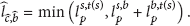
Figure 4 illustrates the time cost of different algorithms. Time cost of local search algorithm and TAG algorithm is the mean time cost of 500 tests. Time cost of genetic algorithm is calculated based on the mean value of iteration step which returns the best solution.

Figure 4

Time cost comparison.

As Figure 4 presents, the genetic algorithm is more time-consuming than the local search algorithm, and the time cost of TAG is minimal. This result is consistent with the theoretical analysis. Additionally, these results clearly show that the time cost of the local search algorithm is linear with the size of candidate set B.

5.3.3. Stability of the Proposed Algorithm

As there is no randomness in the TAG algorithm, each of the 500 tests obtains the same result. For the proposed local search algorithm, there are random steps, so the corresponding result may fluctuate. However, during the tests, we discovered that the result of the proposed algorithm only varies over a small interval; therefore, the proposed algorithm works stably. Table 2 presents the 95% quartile of 500 tests and the 95% confidence interval of the mean value. Regardless of the distribution of the results, the confidence interval of the mean value is still reasonable because of the central limit theorem. Each of the experiments can be treated as an independent random variable, and these independent random variables have the same mean and variance. Thus, the mean value of these independent random variables follows the normal distribution.

Table 2

Stability of proposed algorithm.

M	TAG algorithm results	Mean value of proposed algorithm	95% quartile of proposed algorithm	95% confidence interval of mean value
30	47.2386	47.2386	47.2386	(47.2386, 47.2386)
50	40.9723	40.3376	40.3119	(40.3209, 40.3543)
100	36.4616	35.6586	35.6452	(35.6513, 35.6659)
150	36.4616	34.5786	35.5903	(34.4789, 34.6782)
200	38.0621	34.4447	35.5903	(34.3397, 34.5497)
250	38.0621	34.3215	35.5903	(34.2119, 34.4311)
300	37.105	34.0292	35.9118	(33.9424, 34.1161)
350	37.105	33.9983	35.9118	(33.9132, 34.0835)
400	29.6423	29.0581	29.0172	(29.0222, 29.0940)
450	31.1796	28.4569	28.4420	(28.4423, 28.4715)

As Table 2 presents, the proposed algorithm works quite stably.

5.3.4. Impact of the Number of Overlay Nodes

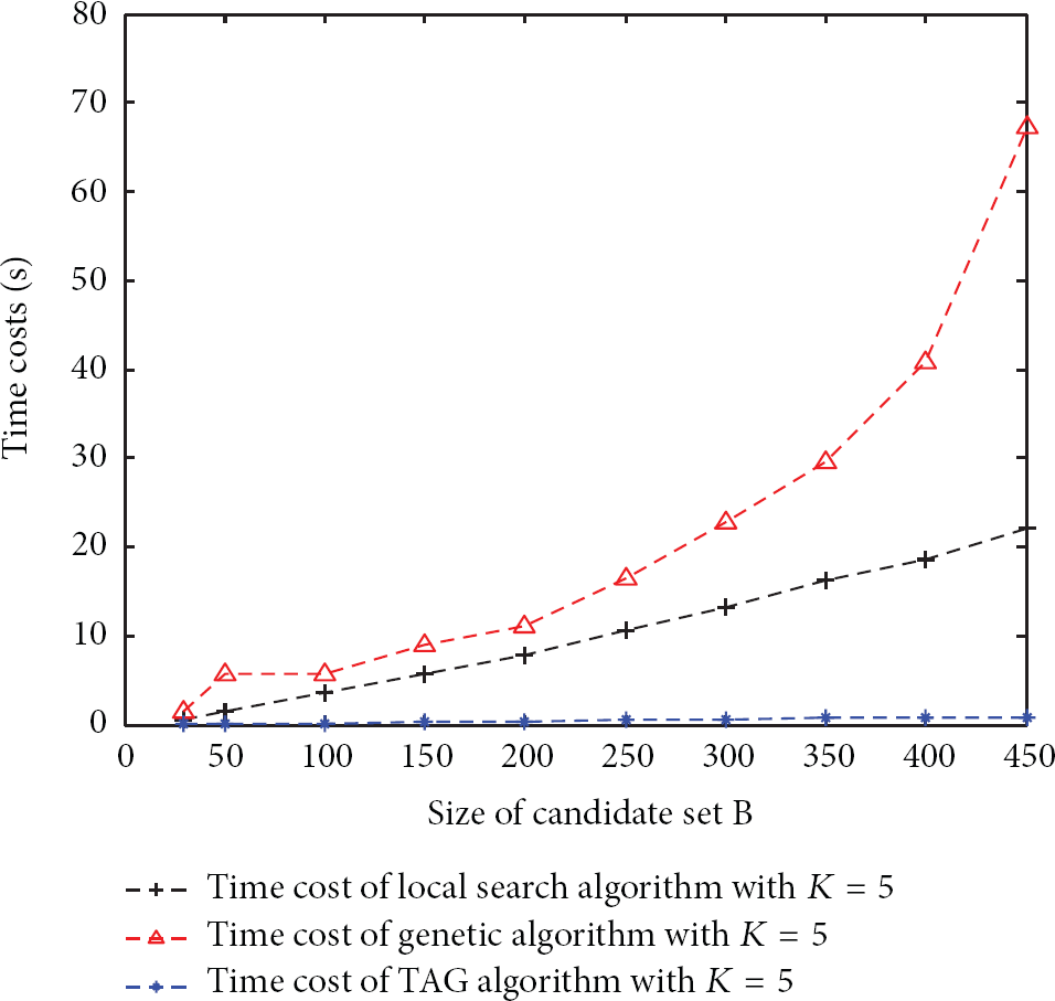
In Section 3, we noted that because of the cost of deploying overlay nodes and the cost of maintaining communication delay information between overlay nodes, the size of set O should be limited. Figures 5 and 6 present the algorithm results and time cost with k increasing under the same M.

Figure 5

Algorithm results with an increasing k.

Figure 6

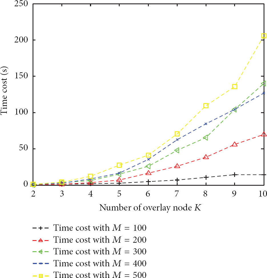
Time cost with an increasing k.

As Figures 5 and 6 show, the algorithm result and the number of overlay nodes are not linearly correlated. When k increases to a certain range, the algorithm results may remain unchanged. In contrast, the time cost will keep increasing. Thus, considering both the algorithm efficiency and cost of deployment, the size of the overlay set should be limited.

6. Experiment with Network Simulation

In this section, the proposed local search algorithm is tested in a network simulation environment. This section is used to represent the algorithm performance and some factors that impact the performance. The network simulator EstiNet is applied.

6.1. EstiNet Network Simulation

EstiNet is a novel network simulator developed by Wang et al. since 1999 [26]. The current version is EstiNet 8.0, which can be found in [10]. A novel simulation methodology called “kernel reentering methodology” is implemented in EstiNet. It combines the advantages of both simulation and emulation. In contrast to existing network simulators NS2 or OPNET, EstiNet uses the real-life UNIX TCP/IP protocol stack during the simulation, and thus all the real-life network application programs can readily run on any node in a simulated network without any modification. This approach can only be performed in emulation mode with other simulators. However, with emulation mode, the performance of switches, links, and so forth, is controlled by the operating system, which makes the results unpredictable; thus, the simulation result cannot be repeated precisely. There is a useful tool in EstiNet called “Generate Large Internet-like Network.” It automatically generates a large network that is similar to the Internet. We use this tool to implement the following experiments.

6.2. Experiment Design

Figure 7 in the following page shows the schematic diagram of the proposed experiment. The red points denote the sensors that are used to collect data. The black points denote the data analyzer used to gather data from sensors. The blue points denote the overlay node, and the red dotted lines denote the logic path from sensor to analyzer through the overlay node. A data-generating program is implemented in each sensor which periodically generates data packets with size L. A data server program is implemented in the analyzer. A data transfer program is implemented in the overlay node, and it retransfers each packet from the sensor to the next overlay node or data server. The goal is to find the optimal overlay node set with given size k that minimizes the sum of time delay from each sensor to the analyzer.

Figure 7

Schematic diagram of the experiments.

In a realistic environment, a delay testing program and transfer program should be placed at each candidate node. Once the optimal overlay set has been found, the transfer program in overlay node is set to continue while the other transfer program suspends. The recalculation should be triggered by time or by network events such as increasing network delay from sensors. For simplicity of analysis, we decompose the progress in the simulation. The simulation steps are as follows. (1)

First, we add network traffic in the simulation environment.

(2)

Then, we find the original time delay from the sensors to the analyzer. In this step, data-generating programs implemented in sensors are directly sending data to the server with the server IP address.

(3)

To obtain the optimal overlay node set, a delay matrix that indicates the time delay of each of the two nodes in candidate set B is needed. Thus, a program to measure time delay from each of the two nodes is required. Here, we use the ping method to acquire the RTT of each of the two nodes. We modified the ping program to calculate the mean RTT and record it in a file.

(4)

We construct the delay matrix out of measured time delay and find the optimal overlay node set.

(5)

We implement the node transfer programs in the overlay nodes and retest the group time delay from the sensors to the analyzer.

The simulation network includes 167 nodes; we randomly select 11 nodes as sensors and 1 node as the analyzer. The overlay node set size is set to 5, and all the other nodes are added into candidate node set. 5 overlay nodes are used because system performance improvement becomes trivial with more overlay nodes. To eliminate the effect of randomness of the network, each of the following experiments has been repeated five times.

6.3. Experimental Results and Analysis

Network communication delay consists of four parts: nodal processing delay, queuing delay, transmission delay, and propagation delay. Queuing delay, nodal processing delay, and propagation delay can be measured by RTT, while transmission delay is related to network bandwidth and data size. To test the overlay network performance with different conditions, different data sizes are used in the experiment. In addition, all the network programs used in the experiment are implemented based on the Linux socket. Within socket programming, a large file should be decomposed into small packet for transfer; otherwise, the delay would increase. Consequently, packet size is also used as a parameter in the experiment. Some interesting phenomena are revealed.

Table 3 illustrates the overlay network performance with increasing data size. Here, D denotes the size of data sent from sensors and P denotes the program transfer packet size. The original cost means the group delay from sensors to analyzer without the overlay. The overlay network cost means the group delay after applying the overlay. The total improvement is calculated with a percentage.

Table 3

Comparison of overlay network performance with increasing data size.

D (Byte)/P (Byte)		Original cost (ms)	Overlay network cost (ms)	Delay improvement (percentage)
$D = 100$	$P = 1000$	48.177	18.186	62.25%
	$P = 1430$	47.968	18.234	61.99%
	$P = 1800$	48.146	18.203	62.19%
$D = 1$ K	$P = 1000$	122.642	101.675	17.10%
	$P = 1430$	122.806	102.589	16.46%
	$P = 1800$	120.466	102.178	15.18%
$D = 5$ K	$P = 1000$	208.380	188.026	9.77%
	$P = 1430$	219.872	180.811	17.77%
	$P = 1800$	300.919	225.573	25.04%
$D = 10$ K	$P = 1000$	372.405	297.364	20.15%
	$P = 1430$	368.939	269.100	27.06%
	$P = 1800$	384.022	276.791	27.92%
$D = 100$ K	$P = 1000$	1521.535	1157.466	23.93%
	$P = 1430$	1543.298	1169.730	24.21%
	$P = 1800$	1526.384	1165.816	23.62%

Table 3 illustrates that overlay network with the proposed algorithm can improve network delay under all conditions. Additionally, the transmission delay would affect system performance. When the sensor data size is small enough, the delay improvement is extremely good. This performance would decrease with the increase of sensor data size. However, after data size achieves a certain range, system performance would be stable. In addition, Table 2 also reveals that the transferring packet size should be set in agreement with MTU. When P is 1430, the system performance is the best. (Although when P is 1800, the delay improvement seems better and the actual delay cost increases.)

6.4. Further Discussion

Although the above experiments show good results of overlay network with the proposed algorithm, there is still work to be done. As described above, the weight of an edge in a network is represented by the average RTT. This weight matrix is the basic requirement for optimization. However, the mean value may not be sufficient to denote this network edge weight matrix. According to current research in internet performance, both internet traffic and delay show the self-similarity characteristic [27, 28]. In a self-similarity time-series, mean value and variance are not appropriate for describing the property because they may not exist [29]. To simulate the effect of hop phenomenon of RTT in real network, a large file is randomly added into network traffic. According to [30], this may be one cause of self-similarity. In Figure 8, the effect of such a phenomenon is shown.

Figure 8

Time cost with random large files.

Figure 8 shows the group delay of 30 former experiments with $D = 5 K$ and $P = 1430$ . It reveals that network delay burst will affect overlay network performance, especially with an IoT application, as the data of an IoT application are generated periodically. As the mean value of RTT is not sufficient for overlay node placement optimization in IoT applications, other parameters such as the Hurst parameter should be imported to define the weight of edges.

7. Conclusions

Network delay is one of the critical issues in IoT applications. Based on both performance and ease of implementation, an internet based dual-layer network, which refers to the overlay network, is suitable for the IoT. Overlay routing has been proved to be a feasible solution to optimize the end-to-end delay. In this work, one of the most important issues in overlay routing, the overlay node placement problem (ONPP), has been discussed. The NP-hardness of multihop k-ONPP has been proven, and a theoretical boundary for k-OPNN optimization is provided.

With defined parameters ω and α, there is no polynomial algorithm with an approximation ratio that is less than $α \times (1 + ((ω - 1) / e))$ . A local search algorithm has been proposed and a theoretical approximation ratio bound has been provided. The approximation ratio of the local search algorithm is less than $ω / α$ . The proposed local search algorithm has been tested and compared with a genetic algorithm and the TAG algorithm with MATLAB tools. The results illustrate that the local search algorithm obtains better performance than the TAG algorithm, and the time cost is linear with the problem scale.

The local search algorithm is finally tested with the network simulator EstiNet. The experimental results show a stable benefit from the proposed method. Moreover, an additional discussion about measuring network edge weight is provided, which reveals a future research direction for ONPP.

Footnotes

Conflict of Interests

The authors declare that there is no conflict of interests regarding the publication of this paper.

Acknowledgments

This work is supported in part by the Ministry of Science and Technology of China under the National 973 Basic Research Program (Grants no. 2013CB228206 and no. 2011CB302505) and the National 863 Science and Technology Support Program (Grant no. 2013BAH19F01), the National Natural Science Foundation of China (Grants no. 61233016), the China Southern Power Grid Science and Technology project (K-SZ2012-026), and the Tsinghua National Laboratory for Information Science and Technology (TNList) cross-disciplinary research program. The authors thank the EstiNet Company for providing a free license for the EstiNet software and technical support.

References

Atzori

Iera

Morabito

The internet of things: a survey

Computer Networks 2010 54 15 2787 2805

2-s2.0-77956877124

10.1016/j.comnet.2010.05.010

Miorandi

Sicari

De Pellegrini

Chlamtac

Internet of things: vision, applications and research challenges

Ad Hoc Networks 2012 10 7 1497 1516

2-s2.0-84860572065

10.1016/j.adhoc.2012.02.016

J. J.

Zhao

WInternet: from net of things to internet of things

Journal of Computer Research and Development 2013 50 6 1127 1134

Chenine

Al Khatib

Ivanovski

Maden

Nordström

PMU traffic shaping in IP-based wide area communication

Proceedings of the 5th International Conference on Critical Infrastructure (CRIS '10)

September 2010

1 6

2-s2.0-78649938101

10.1109/CRIS.2010.5617564

Phadke

A. G.

Thorp

J. S.

Communication needs for wide area measurement applications

Proceedings of the 5th International Conference on Critical Infrastructure (CRIS '10)

September 2010

1 7

2-s2.0-78649953283

10.1109/CRIS.2010.5617484

Chenine

Karam

Nordström

Modeling and simulation of wide area monitoring and control systems in IP-based networks

Proceedings of the IEEE Power and Energy Society General Meeting (PES '09)

July 2009

1 8

2-s2.0-77649297519

10.1109/PES.2009.5275818

Raha

Kamat

Jia

Zhao

Using traffic regulation to meet end-to-end deadlines in ATM networks

IEEE Transactions on Computers 1999 48 9 917 935

2-s2.0-0033340352

10.1109/12.795221

Savage

Collins

Hoffman

Snell

Anderson

T. E.

The end-to-end effects of Internet path selection

ACM SIGCOMM Computer Communication Review 1999 29 4 289 299

10.1145/316194.316233

Roy

Pucha

Zhang

Y. C.

Qiu

Overlay node placement: analysis, algorithms and impact on applications

Proceedings of the 27th International Conference on Distributed Computing Systems (ICDCS '07)

June 2007

53 63

2-s2.0-34848861367

10.1109/ICDCS.2007.127

10.

EstiNet, http://www.estinet.com/

11.

Andersen

D. G.

Balakrishnan

Kaashoek

M. F.

Morris

Resilient overlay networks

Proceedings of the 19th ACM Symposium on Operating Systems Principles (SOSP '01)

2001

131 145

12.

Gummadi

K. P.

Madhyastha

H. V.

Gribble

S. D.

Levy

H. M.

Wetherall

Improving the reliability of internet paths with one-hop source routing

Proceedings of the 6th Symposium on Operating System Design and Implementation (OSDI '04)

2004

183 197

13.

Zhu

Dovrolis

Ammar

Combining multihoming with overlay routing

Proceedings of the 26th IEEE International Conference on Computer Communications (INFOCOM '07)

May 2007

839 847

2-s2.0-34548307286

10.1109/INFCOM.2007.103

14.

Tang

Huai

Zhou

Yin

Chen

A measurement study on the benefits of open routers for overlay routing

Journal of Communications 2009 4 9 714 723

2-s2.0-77958121943

10.4304/jcm.4.9.714-723

15.

Yang

Kim

Y.-A.

Wang

Designing infrastructure-based overlay networks for delay-sensitive group communications

Proceedings of the 50th Annual IEEE Global Telecommunications Conference (GLOBECOM '07)

November 2007

565 570

2-s2.0-39349098466

10.1109/GLOCOM.2007.111

16.

Roy

Pucha

Zhang

Y. C.

Qiu

On the placement of infrastructure overlay nodes

IEEE/ACM Transactions on Networking 2009 17 4 1298 1311

2-s2.0-69249202580

10.1109/TNET.2008.2007433

17.

Cleju

Thomos

Frossard

Network coding node placement for delay minimization in streaming overlays

Proceedings of the IEEE International Conference on Communications (ICC '10)

May 2010

1 5

2-s2.0-77955342855

10.1109/ICC.2010.5502556

18.

Cohen

Raz

Cost effective resource allocation of overlay routing relay nodes

Proceedings of the IEEE International Conference on Computer Communications (INFOCOM '11)

April 2011

3236 3244

2-s2.0-79960884267

10.1109/INFCOM.2011.5935174

19.

Jamin

Jin

Kurc

A. R.

Raz

Shavitt

Constrained mirror placement on the Internet

Proceedings of the IEEE International Conference on Computer Communications (INFOCOM '01)

April 2001

31 40

2-s2.0-0035015620

20.

M.-Y.

Zhu

Shu

Optimal multicast overlay placement for realtime streaming media

Proceedings of the IEEE International Conference on Multimedia and Expo (ICME '04)

June 2004

479 482

2-s2.0-11244281697

21.

Caraguay

L. V. Á.

Peral

A. B.

López

L. I. B.

Villalba

L. J. G.

Software-defined networking: evolution and opportunities in the development IoT applications

International Journal of Distributed Sensor Networks. In press

22.

European Lighthouse Integrated Project, Internet of Things Architecture

http://www.iot-a.eu/public

23.

Pan

Zhu

D.-M.

S.-H.

Xiao

J.-J.

Approximated computational hardness and local search approximated algorithm analysis for k-median problem

Journal of Software 2005 16 3 392 399

2-s2.0-17244375134

10.1360/jos160392

24.

Arya

Garg

Khandekar

Meyerson

Munagala

Pandit

Local search heuristics for k-median and facility location problems

SIAM Journal on Computing 2004 33 3 544 562

2-s2.0-3142776554

10.1137/S0097539702416402

25.

Srinivas

Patnaik

L. M.

Adaptive probabilities of crossover and mutation in genetic algorithms

IEEE Transactions on Systems, Man and Cybernetics 1994 24 4 656 667

2-s2.0-0028409149

10.1109/21.286385

26.

Wang

S. Y.

Chou

C. L.

Huang

C. H.

Hwang

C. H.

Yang

Z. M.

Chiou

C. C.

Lin

C. C.

The design and implementation of the NCTUns 1.0 network simulator

Computer Networks 2003 42 2 175 197

2-s2.0-0037882105

10.1016/S1389-1286(03)00181-6

27.

Leland

W. E.

Taqqu

M. S.

Willinger

Wilson

D. V.

On the self-similar nature of Ethernet traffic

ACM SIGCOMM Computer Communication Review 1993 24 3 183 193

28.

Borella

M. S.

Uludag

Brewster

G. B.

Sidhu

Self-similarity of Internet packet delay

Proceedings of the IEEE International Conference on Communications (ICC '97)

June 1997

513 517

2-s2.0-0030654531

29.

Fractal time series-a tutorial review

Mathematical Problems in Engineering 2010 2010 26

2-s2.0-77951489276

10.1155/2010/157264

157264

30.

Crovella

M. E.

Bestavros

Self-similarity in world wide web traffic: evidence and possible causes

IEEE/ACM Transactions on Networking 1997 5 6 835 846

2-s2.0-0031383380

10.1109/90.650143

Node Placement Analysis for Overlay Networks in IoT Applications

Abstract

1. Introduction

2. Research Background and Related Work

3. Problem Formulation and Analysis

3.1. Problem Formulation

3.2. Problem Analysis

Theorem 1.

Proof.

Theorem 2.

Proof.

4. Proposed Algorithm and Analysis

Algorithm 1: Proposed local search algorithm.

Theorem 3.

Proof.

Theorem 4.

Proof.

5. Algorithm Evaluation

5.1. Experiment Design and Implementation

5.2. Two Other Algorithms for Comparison

5.2.1. Genetic Algorithm

5.2.2. TAG Algorithm

5.3. Experimental Results

5.3.1. Comparison between Optimal Solutions and Genetic Algorithm Solutions

5.3.2. Comparison of Different Algorithms

5.3.3. Stability of the Proposed Algorithm

5.3.4. Impact of the Number of Overlay Nodes

6. Experiment with Network Simulation

6.1. EstiNet Network Simulation

6.2. Experiment Design

6.3. Experimental Results and Analysis

6.4. Further Discussion

7. Conclusions

Footnotes

Conflict of Interests

Acknowledgments

References