Sage Journals: Discover world-class research

Abstract

Several strategies to evaluate the power consumption of of wireless sensor networks (WSNs) have been proposed. The limited amount of energy and the difficulty of recharging them have demanded the emerging of these strategies. However, to evaluate the lifetime of a WSN is not a trivial task due to the complexity of reproducing the environment, inherent dynamism, and complexity and size of WSNs. In this context, we present an approach for evaluating the WSN lifetime by simulating its power consumption using models. This approach consists of a fully automated process for evaluating the WSN lifetime, a set of reusable Coloured Petri Net (CPN) models that express the power consumption of WSN communication protocols, and a strategy for composing CPN models of WSN applications and protocols. In order to assess our power consumption models, we carried out an experimental evaluation that compares the results obtained by simulation against ones existing in the literature.

1. Introduction

Wireless sensor networks (WSNs) consist of dozens, hundreds, or even thousands of small sensors usually collaborating to monitor a particular environment [1]. These sensors are usually deployed into hostile environments (e.g., jungle, high sea, and militarized zones) and are characterized by the scarceness of resources such as energy, storage, and processing capacity. In particular, the limited amount of energy (traditionally supplied by nonrechargeable batteries) and the difficulty of recharging them have demanded the definition of several strategies to allow the evaluation and reduction of power consumption.

The critical aspect in designing and implementing applications and communication protocols for WSN is the limited amount of energy usually available in the motes. Hence, it is needed to adopt the best practices in the development of applications and protocols in order to reduce the power consumption to a minimum. Furthermore, the power consumption of applications and protocols must be evaluated prior to their deployment in the field. This evaluation enable us to estimate the network lifetime, adopt strategies to increase the network lifetime, detect application's power consumption bottleneck, anticipate the time to replace the sensor node batteries, and so on.

The most precise way to evaluate the power consumption of WSNs is periodically measuring the battery level directly on the motes (physical hardware) [2–37]. However, this process has several disadvantages such as the high financial investment, difficulty in reproducing the actual environment, inherent size and dynamism of WSN topology, and the potential impact of hardware and human failures.

Alternatively, the power consumption evaluation of WSNs can be done through adopting models that can be analytically evaluated and/or simulated. As widely known, the use of modelling techniques yields less accurate results than measuring. However, they are characterized by the flexibility and agility to evaluate complex scenarios without interfering in the actual environment. Additionally, the time required to conduct the consumption evaluation can be drastically reduced using models [38].

In this context, this paper presents an approach for evaluating the lifetime of WSNs through models. The key strategy adopted in the proposed solution is to define the consumption models of the application and communication (network) separately. Models that express the power consumption of application commands and protocol actions are defined in CPN (Coloured Petri Net) [16–18]. These models, named basic models, are used to automatically generate the power consumption of the whole application (from a WSN application written in nesC [8]), the network stack (from a WSN topology and configuration parameters), and the WSN node (i.e., from the composition of application and network models). After being generated, these models are used to evaluate the WSN lifetime and the power consumption of each individual WSN node. The whole evaluation process is fully supported by a set of tools that help to develop power-aware applications in nesC and WSN topologies and automatically generate and evaluate power consumption models.

Considering what is being proposed, this paper extends our previous work [5] and has the following unique contributions: (1) a fully automated process for evaluating the WSN lifetime using CPN models, (2) a complete set of reusable CPN power consumption models of WSN communication protocols, and (3) a strategy for composing application and network reusable models. It is worth noting that Petri nets have been widely adopted as a powerful modelling notations used in many different purposes and in several application domains [30, 39] (e.g., evaluating the power consumption of an embedded system [31, 40]).

The rest of this paper is organized as follows. Section 2 introduces basic concepts necessary to understand the rest of the paper. Next, Section 3 presents the proposed solution to evaluate the WSN lifetime. Section 4 carries out an experimental evaluation of the proposed solution, followed by the presentation of related work in Section 5. Finally, last section presents conclusion and future work.

2. Background

Prior to presenting the proposed approach, this section introduces basic concepts of TinyOS, nesC, and Coloured Petri Nets (CPNs).

2.1. TinyOS and nesC

Due to WSN features (mainly limited battery and storage), it is necessary to use an operating system (OS) that works with low power operation and optimizes battery lifetime; beside that, it should manage hardware and abstract its behaviour. TinyOS [24] is one of the most popular OS for WSN that has these features. It was developed in the programming component-based language called nesC [8] (an extension of C), which allows TinyOS to implement hardware drivers (e.g., transceiver) as a component. A component can implement (provider) or use (user) an interface that it is used to connect them (provider and user). WSN application can be quickly programmed choosing components to implement by TinyOS or creating new components. These components are only connected at compile-time, because it can have many providers and the compiled file has only the components needed to run it. Thus, the same WSN application may be deployed in several different motes (e.g., IRIS [28] and MICAz) and the compiled file is optimized for meeting the limited storage of the mote chosen.

2.2. Coloured Petri Nets (CPNs)

Coloured Petri net (CPN) [16–18] is an executable model that combines the capabilities of Petri nets [30–37, 39] and a high-level functional programming language based on Standard ML (known as CPN ML) [29]. CPN has the notion of time and enables us to perform stochastic simulations, which are desired features in performance studies. Meanwhile, CPN ML has primitives for data type definition.

CPN has four main modelling elements, namely, place, token, arc, and transition, as shown in Figure 1.

(i)

Place and token: each place has an identifier (p01), a colour set (INT), and an initial marking (set to 0). The colour set defines the types of tokens that can be stored in the place. The place may also have an initial value, which is used to start the CPN model.

(ii)

Arc: each arc has a single inscription (e.g., i) that is a CPN ML expression. The colour set of the arc expression must match the colour set of the place attached to the arc.

(iii)

Transition: a transition includes an identification (t01), guard, time, and code. The guard is a Boolean expression that must be evaluated to true to enable the transition. When the transition is fired, the code associated with the transition is executed and the time is updated (@+1). The code associated to the transition is divided into three parts: input, output, and action. The action contains the CPN ML code that processes the input (input) and returns a value (output).

Figure 1

Basic elements represented in CPN Tools.

Due to the complexity of creating large nets, a CPN can be broken into smaller pieces through using substitution transitions. These transitions allow the creation of nets with multiple layers of details, where each layer models a different abstraction level that is connected to the next level through the substitution transitions.

The use of the aforementioned feature enables us to divide the model into multiple modules (submodules), where each module has a CPN. Furthermore, it allows the reuse of modules and leads to the reduction of the size of the whole model. The submodules are represented by the substitution transition in the main module. These modules are connected using two places: port (a place in the submodule) and socket (a place in the super module). A socket passes a token to its respective port and vice-versa. There are three kinds of ports: input, which receives a token from the socket; output, which sends a token to the super modules; and I/O that sends and receives tokens.

CPN Tools [29] is a tool that supports Coloured Petri nets. This tool has an interesting mechanism, named monitor, that enables us to observe, inspect, stop, control, and modify the simulation of a CPN model. Four kinds of monitors may be used to stop a simulation (breakpoint), collect simulation data (data collector), and update files during simulation (write-in-files) and for general purpose (user-defined).

3. Evaluating the Power Consumption of WSNs

The proposed approach for evaluating the power consumption of WSNs has followed some basic principles:

(i)

Divide to conquer: the complexity of characterising the power consumption of the whole WSN requires the separation into (i) the consumption of the nesC application (Application layer), (ii) the consumption of the network stack (Network layer), and (iii) the consumption of the WSN node. Application's consumption has also been broken into small pieces, for example, consumption of loop operators, consumption of decision operators, and so on. On the other hand, the consumption of the network is derived from the consumption of individual protocol layers in the network stack, that is, the consumption of the network and link layers;

(ii)

Individual models: consumption models in CPN are created to each element identified in the previous item in such way that the power consumption of the WSN node is defined by composing application and network models;

(iii)

Tool support: Due to the complexity of the power consumption models, the entire process needs to be fully supported by tools in such way that minimum human intervention is necessary. This also helps to reduce the risk of creating incorrect models.

By adopting these principles, Figure 2 shows a general overview of the models and steps needed to obtain the power consumption of WSN nodes. Initially, developers implement an application and define the WSN topology to be evaluated (Creation). This step is assisted by an editor and is made manually. The Language and Protocol Models define the power consumption of small pieces of applications (e.g., language commands) and network protocols (e.g., layer protocols), respectively. These models belong to a proposed library of basic models, which are reusable and may be composed (Composition) in several ways to model different applications (Application Model) and networks stacks (Network Model). Next, the Application model is evaluated and also simplified model (Simplification). Finally, the power consumption model of the WSN node (Node Model) is obtained by integrating the Application and Network models (Integration).

Figure 2

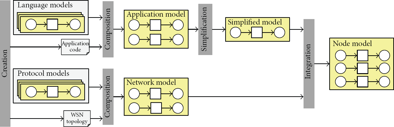
Overview of the proposal.

Next sections present details of the models, the proposed steps, and the tools implemented to support them.

3.1. Power Consumption of the Application Layer

The Language and Application models were partially introduced in [5]. However, these initial models do not include the power consumption due to network, that is, the power consumption represented in these models does include the consumption due to the communication. Figure 3 shows the representation of the Application layer integrated with the Network layer. Some changes in the initial models were necessary for this integration, but they preserved the modelling of the application behaviour.

Figure 3

Schematic view of the Application layer.

Transitions scheduler, sleep, start, end, boot, t1, and tn and places in and out have the same functions as [5]. The transition scheduler is responsible for determining what action (e.g., send packet and collect temperature) is performed. Transitions sleep and boot represent the basic state of the node when it is sleeping (or inactive) and starting, respectively. Transitions start and end are related to the start (set the environment) and end (saving the information simulation), respectively. Transitions t1 and tn represent tasks and events implemented in the application and modelled in a submodule (see Section 2.2). Transition nl was added to make the integration with the Network layer model. This transition models the dispatch of a packet to the network and any activity of the Network layer. Transition receiver represents the action when the node receives a packet. It is worth observing that in the previous version of this model [5], this transition had associated a probability of being triggered to simulate the arrival of a packet. Currently, this transition is triggered when the network layer receives a packet.

These transitions are triggered as follows. Transition scheduler determines that the first transition to be triggered is start, which configures the simulation. Next, transition boot initializes the node application. The next transitions are executed according to the behavior of the application being modeled. The transition scheduler uses a list of actions (called scheduler list) including transitions boot, t1, tn, and nl to determine which transition should be executed. The places in and out represent the beginning and end of an activity, respectively.

3.2. Power Consumption of the Network Layer

The network layer has no power consumption generic model that can be used to represent different network protocols, since there is a great diversity of protocols and characteristics to be modelled. Hence, we designed a pattern (see Figure 4) that any network protocol model must follow. The pattern contains the basic elements that every network layer model (whatever the protocol) must contain. In this way, it is possible to represent any network layer using the same set of elements.

Figure 4

Schematic view of the network layer pattern.

This pattern establishes that any network protocol model must include two places (in and out) to interact with the application (see Section 3.1) and a transition (LinkLayer) that acts like a bridge to the link layer. Places in and out are connected with the Application layer through the places in and out of Figure 3, respectively.

The transition AppPckt represents the creation of a packet by the application (e.g., when the application senses a temperature and needs to send it to the sink node), while the transition CtrlPckt models the creation of a control packet of the protocol, for example, a start-up or setup phase of the protocol. The transition select is responsible for deciding the next node the packet has to be sent to, which it defined by using a list of nodes (place NodeLst). It is worth observing that this pattern does not specify how these routes are defined; this is dependent on the routing algorithm used in the protocol.

When the network layer receives the information (e.g., sensed temperature) from the application layer in place in, the transport layer selects the next node as aforementioned and creates two tokens: one for the application (place out), notifying the transition scheduler of application (Figure 3) to run another transition, and one for the link layer model, indicating that a packet should be sent over the network (place send).

When the network layer receives a packet from the link layer (through transition LinkLayer), it verifies who created the packet. If the packet was created by transition AppPckt (i.e., it comes from the application layer), the network layer fires transition FwdApp that adds an element to the scheduler list (Figure 3), indicating that the transition receive should be performed. If the packet was created by transition CtrlPckt, network layer fires transition ProPckt to process it.

Additionally, the network model can use any energy model. This paper uses the First Order Radio Model 15, which considers power consumption of sending and receiving packets (processing is ignored). In this way, the power consumption of the network model is accounted in the Link Layer (Section 3.3), which is responsible for sending and receiving packets of the environment.

3.2.1. Protocol DIRECT

The protocol DIRECT [35] is ideal for small networks, where nodes have direct communication (single hop) with the sink node. In this case, this protocol does not need to route data through the entire network. Figure 5 illustrates the schematic view of the DIRECT protocol. It is worth observing that in this case, the list of nodes (NodeLst) is not necessary as the nodes have direct communication.

Figure 5

Schematic view of the DIRECT protocol.

When the simulation starts, the sink node sends a message (SinkPckt) to all nodes. Each node, upon receiving this packet, calculates the distance between it and the sink node and modifies the radio range to a minimum necessary that there is communication between them (represented by the transition ProPckt). If the application layer creates a packet (transition AppPckt is fired), the transition FwdApp notifies the application when a packet is available.

3.2.2. Protocol FLOODING

A node using the protocol FLOODING [19] sends a packet in broadcast, where its neighbors will receive the packet and forward it (also in broadcast) until the packet reaches the recipient. It does not need to prepare and store routes to the recipient. Hence, the model of FLOODING (illustrated in Figure 6) also does not need place NodeLst. In this case, transition select only assigns the value broadcast to the packet created.

Figure 6

Schematic view of the FLOODING protocol.

When a node receives the packet, it checks whether the packet is destined to it or not. If so, it forwards the packet to the application (transition FwdApp). Otherwise, it routes the packet to its neighbor (transition RoutePckt).

3.2.3. Protocol GOSSIPING

The protocol GOSSIPING [9], different from protocol FLOODING, chooses a node randomly and forwards the packet to this node (as is illustrated in Figure 7). When the simulation starts (setup phase), all nodes must send a signal (transition SigPckt) in broadcast. When a node receives this packet, it must calculate the distance to the sender and change the node list (place NodeLst).

Figure 7

Schematic view of the GOSSIPING protocol.

When the node creates an application packet (AppPckt), it randomly selects (select) another node and changes the radio range to the minimum necessary to reach the receiver. When a node receives this packet, it checks its destination. If the destination is the current node, the packet is forwarded to the application layer (FwdApp). Otherwise, the packet is sent to another node (RoutePckt), which is chosen randomly.

3.2.4. Protocol LEACH

The protocol LEACH (Low-Energy Adaptive Clustering Hierarchy) [10, 11] is the most popular hierarchical routing of WSNs. This protocol dynamically creates clusters within the network, and the nodes use the cluster heads (CHs) elected as a route to the sink node. From time to time, new nodes randomly become cluster heads. This strategy reduces the energy dissipation among the nodes, increasing the network lifetime. Additionally, this protocol assumes that all nodes can communicate with the sink node directly. These features are modeled in Figure 8.

Figure 8

Schematic view of the LEACH protocol.

This protocol divides its activities into two phases: setup phase and steady phase. The setup phase is used to create the cluster. In the setup phase, all nodes generate a random number between 0 and 1. If the generated value is less than a threshold $T (n)$ , it becomes a cluster head and notifies other nodes (transition NewCHPckt). When nodes receive this notification, they check which is the nearest cluster head (transition CHSelection) and send a packet to the CH chosen to participate in the cluster (transition JoinPckt). In the next step, steady phase, the nodes periodically send a packet to the cluster head (transition AppDataPckt), which aggregates the data received (transition CHAggr) and sends it to the sink node (transition CHDataPckt). After a while, the setup phase starts again (transition NewCHPckt), creating a new cluster.

3.3. Power Consumption of the Link Layer

Similarly to the Network Layer Model, this section presents a pattern (illustrated in Figure 9) to be used as the basis for the link layer protocols, especially, for MAC protocols. It has two places (NetSend and NetReceive) to connect to the network layer and one transition (env) acting as a bridge for the environment. The environment models everything (the medium) between the sender and receiver nodes. Transitions send and receive represent the action of sending and receiving a packet to/from the environment, respectively.

Figure 9

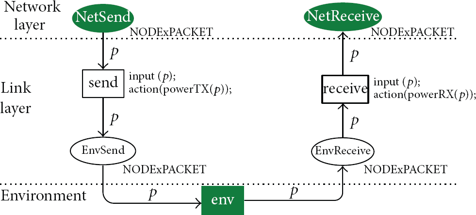
Schematic view of the link layer.

When transition send is triggered, the power consumption is calculated by function powerTX(). Its pseudo-code (due to the complexity of the syntax of CPN ML, we adopted a pseudo-code to facilitate the understanding of the function codes) is shown in Pseudocode 1.

Pseudocode 1

(1)function powerTX(NodexPacket np){

(2) double e1 = eTX * np.getPacketSize();

(3) double e2 = eAMP * np.getPacketSize() * np.getRadioRange()

* np.getRadioRange();

(4) double e = e1+ e2;

(5) long n = np.getNodeId();

(6) addPowerConsumption(n, e);}

This function implements the code presented by Heinzelman et al. [11]. The power consumption of sending a packet (e) is the sum of the power consumption of the transmitter electronics (line 2) and the power consumption of the transmit amplifier (line 3). Furthermore, function addPowerConsumption() increments the power consumption of node n by e.

Similarly, when transition receiver is triggered, the power consumption of receiving a packet is accounted by function powerRX(). It considers that the power consumption of the receiving (line 1) is equal to the power consumption of the receiver electronics (line 2) as shown Pseudocode 2.

Pseudocode 2

(1) function powerRX(NodexPacket np){

(2) double e = EnergyRX * np.getPacketSize();

(3) long n = np.getNodeId();

(4) addPowerConsumption(n, e);}

Finally, this pattern serves as a power consumption model of a MAC layer without collisions and overhearing, that is, a packet is always ready to be sent and all packets received are processed.

3.3.1. Protocol B-MAC

The protocol B-MAC (Berkeley Media Access Control) [32] is one of the best known MAC protocols, because it is very simple. It utilizes CSMA (Carrier Sense Multiple Access) to avoid collision, which is illustrated in Figure 10. This protocol checks (ChckEnv) whether the environment is free or not before sending a packet. If the environment is busy (place busy), the node waits for a random time (transition wait) before trying to send the packet again. If no node is transmitting (place free), it sends the packet (transition send).

Figure 10

Schematic view of the B-MAC protocol.

When a node receives a packet (transition receive), it checks the packet destination. If the destination is the current node, the packet is forwarded to the upper layer (place NetReceive). Otherwise, it considers an overhearing (place overhearing) and ignores the packet (transition discard).

3.4. Environment Model

The environment models everything (the medium) between sender and receiver nodes in such way that it identifies, at runtime, the connections among the nodes and forwards the packet from one node (sender) to another (receiver). In Figure 11, the places send and receive represent when a node sends and receives a packet, respectively. As mentioned before, transition env models everything between the nodes.

Figure 11

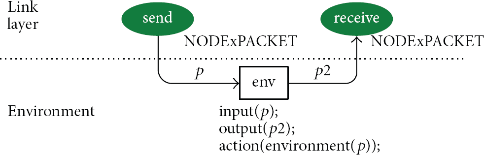
Schematic view of the environment.

3.5. Power Consumption of the Node

The power consumption model of the WSN node is obtained by combining the Application and Network (Network and Link layers) models. Due to the size and complexity, it is unfeasible to simulate the power consumption of the combined model. Hence, to solve this problem, it is necessary initially to simulate the application model and obtain its power consumption. The data obtained through simulation are used in the reduced model (illustrated in Figure 12) to simulate the application model. The transition PwrConsumption models the consumption of the whole Application layer. In this way, the network model considers aspects of the application without changing its structure and behaviour.

Figure 12

Simplified model representing the power consumption of the application.

3.6. Tools

In order to support the whole process shown in Figure 2, a set of tools was designed and implemented. Figure 13 presents a general overview of the proposed environment and its basic elements, namely, an editor (IDEA4WSN), a translator (Sensor2Model), an Evaluator and model repositories (Language and Protocol models). The editor is mainly used to implement WSN energy-aware applications and create WSN projects (topology and protocols). The translator is responsible for the Composition, Simplification, and Integration steps (see Figure 2). The Application model is generated from the application code (e.g., nesC), whilst the Network model is obtained from the WSN topology. Next, these models are integrated, creating the Node model. The Evaluator takes the Node model and produces the amount of energy consumed by the whole WSN. Finally, the repositories store CPN basic models used to compose the Application and Network models.

Figure 13

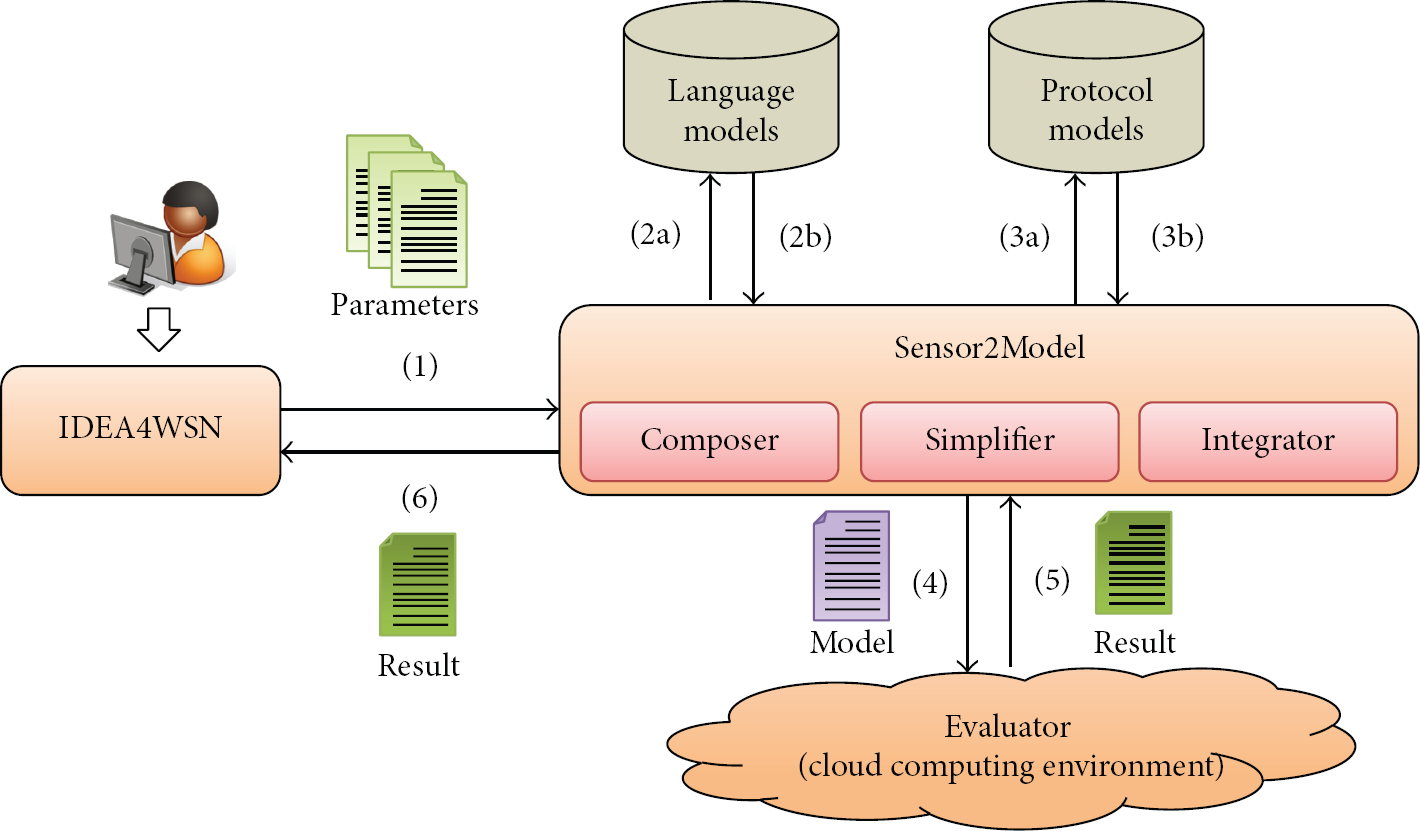
Overview of the tools set implemented.

This figure also illustrates the operation of the three tools together. First, the user creates an application or network project in the editor. Next, some parameters (e.g., application directory, topology file, hardware platform, level of confidence, and others) are passed to the translator (1) that creates the power consumption model by accessing the repository of basic models (2a/3a and 2b/3b). After this step, the model is passed to the simulator (4). When the simulation finishes, the power consumption results are passed to the translator (5), which forwards them to the editor (6) that shows the results through a WSN energy map as shown in Figure 14.

Figure 14

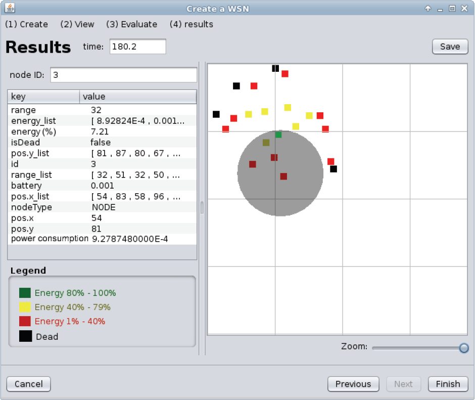
Energy map of a WSN with 21 sensor nodes.

These tools were implemented in Java, the editor was integrated with Eclipse IDE [7], and the Evaluator was deployed in Amazon EC2 (cloud).

4. Experimental Evaluation

This section has two main objectives: to validate the automatically generated network models and to show the impact of the application on the WSN lifetime. To perform the evaluation, we have defined three experiments:

(i)

Experiment 1. It shows the WSN lifetimes obtained using the proposed network models and compares them against results found in literature. The WSN lifetime was measured using four different communication protocols (LEACH, GOSSIPING, DIRECT, and FLOODING). In this experiment, the power consumption of each WSN node is only due to the network stack and no application runs in the node;

(ii)

Experiment 2. It shows the impact of an application on the WSN lifetime considering different communication protocols (same protocols of Experiment 1). In this experiment, the power consumption of WSN nodes is due to the application and the network stack;

(iii)

Experiment 3. It shows the impact of different applications on the WSN lifetime considering only one communication protocol. In this experiment, the power consumption of WSN nodes is due to the application and network stack.

4.1. Stopping Criteria

In all aforementioned experiments, we have adopted two kinds of stopping criteria: ones related to the simulation time and ones related to the reliability of the results obtained through the simulation. First kind of criteria defines when the simulation needs to stop (single execution of the model). For example, the simulation should stop when the first WSN node goes down as its battery runs out. This criterion is known as FND (first node dies). Similar criteria include LND (last node dies), PND (percentage of nodes die), and HND (half nodes die). On the other hand, the second criteria define whether the results obtained after stopping the simulation are reliable or not. In the case the expected reliability is not reached, the simulation is executed again.

The criterion of reliability adopted is the called batch means. It divides n executions of the model into parts (called batch) with similar sizes. Next, it computes the average of each batch and constructs a list (called batch means) with these averages. We can determine the error of the simulation through batch means. The error is calculated with the following equation:

\begin{matrix} E = \frac{t^{(k - 1,1 - α)} \times s}{\sqrt{k}}, \end{matrix}

(1)

where t is the value of the T-Student distribution with degree of freedom $k - 1$ and level of confidence (defined by user) equal to $1 - α$ ; k is the size of the batch means and s is the standard deviation of the batch means. We compare the error of the batch means (E) with a value defined by the user, called “max error.” The simulation stops when E is less than or equal to the max error.

4.2. Configuration

The network model uses the First Order Radio Model [11], which accounts the power consumption when the sensor node sends and receives a packet. In this case, the power consumption of CPU, EEPROM, and LEDs is not considered.

The network consists of 20 sensor nodes and 1 sink node. The WSN sensor nodes are randomly distributed in an area of 400 × 400 m. The position of the sensor nodes lies in the interval of 10–50 m to the sink node position. The radio range is 200 m and the node's energy level is 1 mJ in the first experiment and 10 J in the other. Regarding the adopted protocols, we selected the protocols DIRECT, FLOODING, GOSSIPING, and LEACH as they are widely documented and used in WSNs. Their settings are the same as ones presented in Senouci et al. [35].

4.3. Results

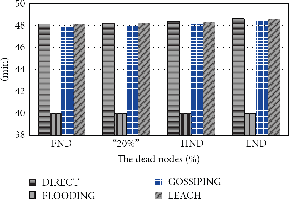
In the first experiment, similar to one carried out by Senouci et al. [35], the application sends a packet every 2 seconds and the WSN node initial energy is set to 1 mJ.

Figure 15 shows the percentage of dead nodes (because battery runs out) over time obtained through the simulation model. As expected, the FLOODING has the worst performance. The GOSSIPING performed better than the FLOODING around 3x and 6x to the stop criteria FND and LND, respectively. This occurs because the FLOODING sends a packet to all nodes, while GOSSIPING forwards it to just one node. The DIRECT protocol had worse performance than the LEACH in the first three criteria (FND, HND, and 20%) because the farthest nodes die earlier. However, in the last criterion (LND), it had a better performance. Certainly, the nonuniform distribution of cluster heads (CHs) affects negatively the power consumption of WSN. For example, the number of CH does not remain the same over time and it is difficult to keep CHs present in all parts of the network. Consequently, some WSN nodes spend more energy due to the absence of CHs close to them. These results are similar to ones obtained by Senouci et al. [35] except for the criterion HND, in which DIRECT had a better performance than the LEACH.

Figure 15

Dead nodes behavior (Experiment 1).

As aforementioned, Experiment 2 simulates an application running atop different communication protocols and evaluates its impact on the WSN lifetime. This application senses temperature every 2 seconds and sends it to the sink node. The settings of this experiment are similar to the previous one except for the initial energy level that is set to 10 J (it was 10 mJ in Experiment 1). This was necessary because the WSN node now executes an application in addition to the network stack and this application consumes a greater amount of energy. Figure 16 shows the dead nodes behaviour of Experiment 2.

Figure 16

Dead nodes behavior (Experiment 2).

The power consumption of WSN nodes has a similar behaviour to Experiment 1. It means that the protocol having a good performance in Experiment 1 still has the same consumption pattern in Experiment 2 despite the existence of the application. Hence, the integration of Network and Application models (see Section 3.5) preserves the power consumption patterns of communication protocols found in Experiment 1.

The last experiment was created to show the impact of the application behaviour on the WSN lifetime. With this purpose in mind, we developed three applications that collect temperature (every 2 seconds) and send it to the sink node. The first application (App 1) sends a temperature immediately after capturing it. The second application (App 2) sends the average of five sensed temperatures. The last application (App 3) only sends data when the temperature exceeds a certain value. In this case, it was considered that in 30% of cases the temperature exceeds this value. Additionally, the protocol DIRECT was chosen because it has the best performance among the protocols in the previous experiments.

As expected, App 1 has the worst result (see Figure 17) because it sends a message immediately after collecting the temperature. App 3 had the best performance in all criteria, due to two factors. (1) It has little processing after capturing the temperature and (2) it only sends a message when is needed. App 2 had an average performance due to data aggregation, which helps to save energy. In this case, it was not advantageous to aggregate little data (five measurements only). Surely, aggregation with more data would increase the lifetime of the sensor node and, consequently, the network lifetime.

Figure 17

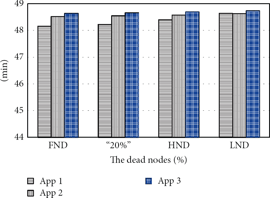
Dead nodes behavior (Experiment 3).

5. Related Work

In this section, we present and compare existing approaches for evaluating the power consumption of WSN networks. These approaches have been grouped considering the adopted evaluation technique (measurement, simulation, and analytical modelling).

5.1. Measurement

The adoption of measurement techniques depends on assembling the environment to perform the proper measurements: the application, the WSN motes (e.g., IRIS and MICAz) to deploy the application, the power supply (e.g., Icel Manaus PS-1500) to maintain the constant voltage of the WSN mote, one oscilloscope (e.g., Agilent DSO3102A) for data measurement, and one program that collects and processes data from the oscilloscope (e.g., AMALGHMA [41]).

One limitation of using measurement techniques is the setting-up of the aforementioned environment, which is composed of several elements. For that reason, it is usual to evaluate the impact of encryption algorithms (e.g., RC5, RSA) [2], the middleware (e.g., POCOBOS) [13], and the operating system (e.g., TinyOS, Contiki) [22] on the application's power consumption in a single WSN node. In these cases, some approaches [20] take for granted that the power consumption of the whole network may be deduced from the measured consumption of this individual node as the nodes usually have the same configurations (e.g., application, mote, operating system, and so on).

5.2. Simulation

Simulation approaches mainly focus on defining and simulating models of architectures (hardware platform), operating systems, and applications. For example, AVRORA [42] has been used to evaluate the power consumption of MICA mote family [12]. Somov et al. [43] present a simulation framework to estimate the power consumption of WSN applications for arbitrary hardware platforms. Similarly, TOSSIM [23] has also been used to compare the network lifetime (consequently, power consumption) when using different communication protocols. For example, Senouci et al. [35] and Iyer et al. [15] evaluate the power consumption of the protocol EHEED and a generic transport layer protocol (STCP), respectively.

Unlike the aforementioned approaches that simulate directly the programming code, existing researches also concentrate on defining behavioural models of WSNs. Shareef and Zhu [36] use Deterministic and Stochastic Petri Nets (DSPNs) to model the behaviour of IMote2's CPU and radio. NS-2 [14] and OPNET [3] have also been used to evaluate the power consumption of WSNs. Mainly, the NS-2 is widely adopted to simulate the behaviour of WSNs with different protocols such as LEACH, TEEN, and APTEEN [26]; AODV, DSDV, and DSR [21], and S-MAC and RMAC [6]. However, the behaviour of the application (and its power consumption) is not as important as the protocols.

Finally, our previous paper [5] presented an approach for evaluating the power consumption of WSN applications by using simulation models along with a set of tools to automate the proposed approach. Starting from a programming language code, we automatically generate consumption models used to predict the power consumption of WSN applications. In order to evaluate the proposed approach, we compared the results obtained by using the generated models against ones obtained by measurement. It is worth observing that our previous paper [5] focused on the application, whilst this paper concentrates on the power consumption of the communication infrastructure used by the application. Due to the inherent differences between applications and network protocols, the proposed models and the way they are generated is completely different in both cases.

Most of these applications are strongly coupled to a particular hardware platform, which makes the adoption of the same simulation mode for different WSN motes difficult. In particular, our solution facilitates the evaluation of new platforms, as the presented models are generic and only need to be configured to a particular mote. Another advantage of the proposed approach is the generation of power consumption which results from a programming language code in an automatic way. Furthermore, most studies evaluate the behaviour of the application and of the network at the same time, delaying to finalize the evaluation. This study developed a sequence of steps to integrate and improve the evaluation of the application with the network.

5.3. Analytical Modelling

Current proposals that use analytical modelling are related to a part of our proposal: the network. The other two parts (application and integration) are more common in the measurement and in the simulation than in analytical modelling. For example, Asmussen and Glynn [44] estimated the lifetime of particular WSN motes developed by them; Rusli et al. [33] evaluated the performance of the Opportunity Routing (OR) protocol [45]; Manjeshwar et al. [27] modelled, evaluated, and compared the energy consumption of two protocols, namely, LEACH [10, 11] and APTEEN [26]; Sahota et al. [34] proposed and evaluated a new MAC protocol name DS-MAC [25]; and Cano et al. [46] verify the benefits (overhearing and collision) of Low Power Listening (LPL) [12] of MAC protocols.

In practice, these analytical models used to evaluate the power consumption of WSNs are strongly coupled to a particular network element, for example, routing protocol and MAC protocol. Hence, a new model needs to be developed if the WSN uses a different routing or MAC protocol. This paper has not this limitation because we propose a sequence of steps to create a customized WSN power consumption model (see Section 3). This sequence of steps creates a model with all factors (e.g., packet size, energy level, number of sensor nodes, routing protocol, and MAC protocol) chosen by the user.

6. Conclusion and Future Work

This paper presented a fully automated process for evaluating the power consumption of WSNs. Basic in the proposed process is the set of models that define the power consumption of communication protocols used in the link and network layers. These models are reusable and were composed with application models to express the power consumption of WSN nodes. The application model is evaluated and a simplified model is used to represent its power consumption. Next, the power consumption model of the WSN node (Node Model) is defined by integrating the Application and Network models. Finally, the node models are simulated to evaluate the WSN lifetime.

The main contributions of this paper are the set of reusable power consumption models of network protocols, their integration with the application models, and the set of tools that support the entire evaluation process. The performed experiments showed that the network model returned data similar to ones found in the literature. Additionally, the experiments illustrated the performance loss of the WSN nodes when considering the power consumption of the application. They also showed that the application settings could increase the lifetime of the network.

For future work, we are starting to develop more models to assess other aspects of the WSN like dependability. Meanwhile, in addition to application and network stack, we are envisioning the modelling of middleware components and their impact on the power consumption of WSNs.

Footnotes

Conflict of Interests

The authors declare that there is no conflict of interests regarding the publication of this paper.

Acknowledgments

This work has been partially supported by the “Fundação de Amparo à Ciência e Tecnologia do Estado de Pernambuco” (FACEPE) through the process number IBPG-0396-1.03/10.

References

Agre

Clare

An integrated architecture for cooperative sensing networks

Computer 2000 33 5 106 108

Chang

C.-C.

Nagel

D. J.

Muftic

Assessment of energy consumption in wireless sensor networks: a case study for security algorithms

Proceedings of the IEEE Internatonal Conference on Mobile Adhoc and Sensor Systems (MASS ′07)

October 2007

1 6

2-s2.0-50249146919

10.1109/MOBHOC.2007.4428758

Chang

Network simulations with OPNET

Proceedings of the Winter Simulation Conference Proceedings

December 1999

307 316

2-s2.0-0033311578

CPN Tools http://cpntools.org/

Dâmaso

Freitas

Rosa

Silva

Maciel

Evaluating the power consumption of Wireless Sensor Network applications using models

Sensors 2013 13 3 3473 3500

2-s2.0-84875145577

10.3390/s130303473

Shu

Saha

A. K.

Johnson

D. B.

RMAC: a routing-enhanced duty-cycle MAC protocol for wireless sensor networks

Proceedings of the 26th IEEE International Conference on Computer Communications (INFOCOM ′07)

May 2007

1478 1486

2-s2.0-34548317545

10.1109/INFCOM.2007.174

Eclipse Foundation

Eclipse Standard 4.3

http://www.eclispe.org

Gay

Welsh

Levis

Brewer

von Behren

Culler

The nesC language: a holistic approach to networked embedded systems

Proceedings of the ACM SIGPLAN Conference on Programming Language Design and Implementation

June 2003

ACM

1 11

2-s2.0-0037702249

Hedetniemi

S. M.

Hedetniemi

S. T.

Liestman

A. L.

A survey of gossiping and broadcasting in communication networks

IEEE Networks 1988 18 4 319 3349

10.

Heinzelman

Application-Specific Protocol Architectures for Wireless Networks [Ph.D. thesis] 2000

Boston, Mass, USA

Massachusetts Institute of Technology

11.

Heinzelman

W. R.

Chandrakasan

Balakrishnan

Energy-efficient communication protocol for wireless microsensor networks

Proceedings of the 33rd Annual Hawaii International Conference on System Siences (HICSS ′00)

January 2000

3005 3014

2-s2.0-0033877788

12.

Hill

J. L.

Culler

D. E.

Mica: a wireless platform for deeply embedded networks

IEEE Micro 2002 22 6 12 24

2-s2.0-0036870095

10.1109/MM.2002.1134340

13.

Hiltunen

Ala-Louko

Taumberger

Experimental performance evaluation of POBICOS middleware for wireless sensor networks

ISRN Communications and Networking 2012 2012 10

180369

10.5402/2012/180369

14.

The Network Simulator—NS2

ISI, University of Southern California, Los Angeles, Calif, USA, http://www.isi.edu/nsnam/ns

15.

Iyer

Y. G.

Gandham

Venkatesan

STCP: a generic transport layer protocol for wireless sensor networks

Proceedings of the 14th International Conference on Computer Communications and Networks (ICCCN ′05)

October 2005

449 454

2-s2.0-33748361370

10.1109/ICCCN.2005.1523908

16.

Jensen

Kristensen

Coloured Petri Nets 2009

New York, NY, USA

Springer

Modelling and Validation of Concurrent Systems

17.

Jensen

Coloured Petri Nets: Basic Concepts, Analysis Methods and Practical Use, Vol. 2 1995

London, UK

Springer

18.

Jensen

Kristensen

L. M.

Wells

Coloured Petri Nets and CPN Tools for modelling and validation of concurrent systems

International Journal on Software Tools for Technology Transfer 2007 9 3-4 213 254

2-s2.0-34249933531

10.1007/s10009-007-0038-x

19.

Y. B.

Choi

J. M.

Kim

J. H.

Kahng

H. K.

Goto

A new directional flooding protocol for wireless sensor networks

Formation Networking. Networking Technologies for Broadband and Mobile Networks 2004

Berlin, Germany

Springer

93 102

20.

Kohvakka

Hannikainen

Hamalainen

Wireless sensor network implementation for industrial linear position metering

Proceedings of the 8th Euromicro Conference on Digital System Design

2005

267 273

21.

Kulkarni

Prasad

Cornean

Gupta

Performance evaluation of AODV, DSDV and DSR for quasi random deployment of sensor nodes in wireless sensor networks

Proceedings of the International Conference on Devices and Communications (ICDeCom ′11)

February 2011

1 5

2-s2.0-84858133667

10.1109/ICDECOM.2011.5738571

22.

Lajara

Pelegrí-Sebastiá

Perez Solano

J. J.

Power consumption analysis of operating systems for wireless sensor networks

Sensors 2010 10 6 5809 5826

2-s2.0-77954806223

10.3390/s100605809

23.

Levis

Lee

Welsh

Culler

TOSSIM: accurate and scalable simulation of entire TinyOS applications

Proceedings of the 1st International Conference on Embedded Networked Sensor Systems (SenSys ′3)

November 2003

ACM

126 137

2-s2.0-18844399081

24.

Levis

Madden

Polastre

Szewczyk

Whitehouse

Woo

Gay

Hill

Welsh

Brewer

Culler

Weber

Rabaey

J. M.

Aarts

TinyOS: an operating system for sensor networks

Ambient Intelligence 2005

Berlin, Germany

Springer

115 148

25.

Lin

Qiao

Wang

Medium access control with a dynamic duty cycle for sensor networks

Proceedings of the IEEE Wireless Communications and Networking Conference (WCNC ′04)

March 2004

1534 1539

2-s2.0-4544278757

26.

Manjeshwar

Agrawal

APTEEN: a hybrid protocol for efficient routing and comprehensive information retrieval in wireless sensor networks

Proceedings of the International Parallel and Distributed Processing Symposium (IPDPS ′02)

2002

195 202

27.

Manjeshwar

Zeng

Q.-A.

Agrawal

D. P.

An analytical model for information retrieval in Wireless Sensor Networks using enhanced APTEEN protocol

IEEE Transactions on Parallel and Distributed Systems 2002 13 12 1290 1302

2-s2.0-0036964041

10.1109/TPDS.2002.1158266

28.

MEMSIC

Wireless Module Iris: Iris Datasheet

http://www.memsic.com

29.

Milner

Tofte

Macqueen

The Definition of Standard ML 1997

Cambridge, Mass, USA

The MIT Press

30.

Murata

Petri nets: properties, analysis and applications

Proceedings of the IEEE 1989 77 4 541 580

2-s2.0-0024645936

10.1109/5.24143

31.

Nogueira

Vasconcelos Neto

Maciel

Lima

Barreto

Embedded systems'software performance and energy consumption by probabilistic modeling: an approach based on coloured petri nets

Petri Nets and Other Models of Concurrency 2006 4024

Berlin, Germany

Springer

261 2281 Lecture Notes in Computer Science,

32.

Polastre

Hill

Culler

Versatile low power media access for wireless sensor networks

Proceedings of the 2nd International Conference on Embedded Networked Sensor Systems (SenSys ′04)

November 2004

ACM

95 107

2-s2.0-26444451023

33.

Rusli

M. E.

Harris

Punchihewa

Markov Chain-based analytical model of opportunistic routing protocol for wireless sensor networks

Proceedings of the IEEE Region 10 Conference (TENCON ′10)

November 2010

257 262

2-s2.0-79951668322

10.1109/TENCON.2010.5686003

34.

Sahota

Kumar

Kamal

A wireless sensor network for precision agriculture and its performance

Wireless Communications and Mobile Computing 2011 11 12 1628 1645

2-s2.0-84555187658

10.1002/wcm.1229

35.

Senouci

M. R.

Mellouk

Senouci

Aissani

Performance evaluation of network lifetime spatial-temporal distribution for WSN routing protocols

Journal of Network and Computer Applications 2012 35 4 1317 1328

2-s2.0-84860384745

10.1016/j.jnca.2012.01.016

36.

Shareef

Zhu

Energy modeling of wireless sensor nodes based on Petri nets

Proceedings of the 39th International Conference on Parallel Processing (ICPP ′10)

September 2010

101 110

2-s2.0-78649531333

10.1109/ICPP.2010.19

37.

Shinghal

Noor

Srivastava

Singh

Power measurements of Wireless Sensor Network node

International Journal of Computer Engineering and Science 2011 1 1 8 13

38.

Yeap

Practical Low Power Digital VLSI Design 1998

Boston, Mass, USA

Kluwer Academic

39.

Silva

Terue

Colom

Reisig

Rozenberg

Linear algebraic and linear programming techniques for the analysis of place/transition net systems

Lectures on Petri Nets I: Basic Models 1998

Berlin, Germany

Springer

309 373

40.

Callou

MacIel

Tavares

Andrade

Nogueira

Araujo

Cunha

Energy consumption and execution time estimation of embedded system applications

Microprocessors and Microsystems 2011 35 4 426 440

2-s2.0-79955554419

10.1016/j.micpro.2010.08.006

41.

Tavares

Silva

Maciel

An environment for measuring and scheduling time-critical embedded systems with energy constraints

Proceecings of the 6th IEEE International Conference on Software Engineering and Formal Methods (SEFM ′08)

November 2008

291 300

2-s2.0-58049141176

10.1109/SEFM.2008.47

42.

Titzer

B. L.

Lee

D. K.

Palsberg

Avrora: scalable sensor network simulation with precise timing

Proceecings of the 4th International Symposium on Information Processing in Sensor Networks (IPSN ′05)

April 2005

477 482

2-s2.0-33744909363

10.1109/IPSN.2005.1440978

43.

Somov

Minakov

Simalatsar

Fontana

Passerone

A methodology for power consumption evaluation of wireless sensor networks

Proceecings of the IEEE Conference on Emerging Technologies and Factory Automation (ETFA ′09)

September 2009

1 8

2-s2.0-77949886482

10.1109/ETFA.2009.5347152

44.

Asmussen

Glynn

P. W.

Stochastic Simulation: Algorithms and Analysis 2007

New York, NY, USA

Springer

45.

Biswas

Morris

Opportunistic routing in multi-hop wireless networks

ACM SIGCOMM Computer Communication Review 2004 34 1 69 74

46.

Cano

Bellalta

Barceló

Oliver

Sfairopoulou

Analytical model of the LPL with wake up after transmissions MAC protocol for WSNs

Proceedings of the 6th International Symposium on Wireless Communication Systems (ISWCS ′09)

September 2009

146 150

2-s2.0-71449097501

10.1109/ISWCS.2009.5285320

Using Coloured Petri Nets for Evaluating the Power Consumption of Wireless Sensor Networks

Abstract

1. Introduction

2. Background

2.1. TinyOS and nesC

2.2. Coloured Petri Nets (CPNs)

3. Evaluating the Power Consumption of WSNs

3.1. Power Consumption of the Application Layer

3.2. Power Consumption of the Network Layer

3.2.1. Protocol DIRECT

3.2.2. Protocol FLOODING

3.2.3. Protocol GOSSIPING

3.2.4. Protocol LEACH

3.3. Power Consumption of the Link Layer

Pseudocode 1

Pseudocode 2

3.3.1. Protocol B-MAC

3.4. Environment Model

3.5. Power Consumption of the Node

3.6. Tools

4. Experimental Evaluation

4.1. Stopping Criteria

4.2. Configuration

4.3. Results

5. Related Work

5.1. Measurement

5.2. Simulation

5.3. Analytical Modelling

6. Conclusion and Future Work

Footnotes

Conflict of Interests

Acknowledgments

References