Feasibility Study on the Implementation of Cubic Motion Curve for Vehicle Trajectory Planning

Abstract

Cubic Motion curve has been introduced to integrate the information of path and motion. Since this is a new approach, a feasibility study has been carried out to analyse the practicality of Cubic Motion curves used as the input for the study of vehicle dynamic response. This study requires the development of three modules, namely, the Cubic Motion module, the vehicle dynamic model, the driver model (VDM-DM) module, and, lastly, the integrated module. The Cubic Motion module will generate Cubic Motion curve. The VDM-DM module applies the 2 DOF bicycle model and links it with Reński's driver model. Finally, an integrated module will merge both previous modules as a complete system for trajectory and vehicle response as the output. The double lane change and the Slalom test were the case studies used to develop an understanding of the applicability of the three types of Cubic Motion input, namely, natural, adjusted tangent, and additional vertex cubic motion. The finding of this study is that Cubic Motion is in fact a compact representation of curve with motion attributes and can be directly associated with a vehicle dynamic response study.

1. Introduction

Trajectory planning depends on the ability of the vehicle to steer according to the planned trajectories. Some works take only path into account without considering the vehicle dynamic effect [1–4]. Kala and Warwick [5], however, looked into possibility of implementing trajectory planning using real time assessment. A real time genetic algorithm with Bezier curves for trajectory planning was adopted.

In 2008, Braghin et al. [6] extended the work on trajectory planning by taking into account the vehicle dynamic effect. Based on the geometry of the race track, the shortest part, with the least curvature path, and speed profile were developed. The race car driver model was used to manoeuvre through the path. Yuan-Yuan et al. [7] used the vehicle dynamic on the curved road with the aim of developing theoretical support to design a suitable curved road and alignment as well as management of counter flow conflicts. Guo et al. [8] used the trapezoidal acceleration profile for the curved road. Finally, the desired and actual displacement can be compared and the steering angle required can be obtained.

The requirement of having two inputs, trajectory, and motion attributes becomes essential when the study is related to vehicle responses [6–8]. Therefore, most of the current research must separately input both entities. This can be improved by having both entities as a single input. This is accomplished through the introduction of a new type of curve, which is formed by the integration of cubic spline and dynamic of motion, which is called Cubic Motion. Cubic spline will draw the path, while dynamic of motion will position the vertices.

The development of Cubic Motion is based on the need to have the path and motion to develop a compact representation for bringing road safety study to the desktop. Prior to full-fledged implementation in the context of the road safety study, a feasibility study must first be carried out to fully understand the applicability of the Cubic Motion curve.

As an exploratory study, the focus of the research is to use the Cubic Motion curve as the input to the vehicle dynamic model (VDM) and driver model. VDM will predict the dynamic responses of the vehicle resulted from vehicle maneuvering to follow the designated path, while the driver model will act as a driver to make the vehicle travel according to the designated path. Therefore, this paper will explore the applicability of the Cubic Motion curve used as the input for the VDM and driver model. This study will explore the practicality of the three different types of Cubic Motion curve.

The next section will describe the methodology used to develop the system. The results of two case studies, a double lane change (DLC) and slalom test, are discussed in Section 3. The discussion and conclusion will be in Sections 4 and 5, respectively.

2. Methodology

Figure 1 shows the methodology adopted in the development of the system, which is implemented using a modular approach. The modular approach comprises three modules which are as follows.

• Cubic Motion module: this module will create the Cubic Motion curve. The user needs to define the number of control points (N) and their coordinates (P) together with the velocity (V) of the vehicle.

• VDM-DM module: this module comprises the vehicle dynamic and driver models. The bicycle model is used for vehicle dynamic calculation and Andrej Reński's Driver model is used for the driver model. Both models are verified prior to being linked with the Cubic Motion module.

• Integrated module: finally, this module will integrate both modules into a complete system. The Cubic Motion curve will provide the intended trajectory, initial yaw angle, and velocity. Meanwhile, the sight length will be set by the user.

Figure 1:

System development methodology.

2.1. Cubic Motion Module

This module will develop Cubic Motion curve. A three-step procedure is adopted, which is as follows:

• development of the cubic spline curve;

• integration of the cubic spline and dynamic of motion;

• analyzing the error.

2.1.1. Development of the Cubic Spline Curve

Hermite curves are the basis for the development of the cubic spline. When a number of Hermite curves are joined together, they will form the cubic spline. For n control points, there are n − 1 Hermite curves to form the cubic spline. To ensure smoothness at the joints, the first and second derivatives at two adjacent Hermite curves must be equal. This equality will resolve the tangent of the control points, although the tangent of the first and last control points remains unknown.

Assuming the second derivative of the first and last vertices is equal to zero, natural cubic spline is generated and when motion attribute is inserted into the curve, it will transform to natural Cubic Motion. This will be one of three curves studied in this research. The remaining curves are adjusted tangent and additional vertex cubic spline. These three curves will be later transformed into respective Cubic Motion curve. In the following section, all three types of curves will be described. For the theoretical background of the Hermite curve and cubic spline; refer to Anand [9].

Natural Cubic Spline. In the generation of the natural cubic spline, the tangent of the control points must be calculated first. Equation (1) calculates the tangents of the control points:

$\left[\begin{array}{c}{P}_{\mathrm{0}}^{\prime }\\ P_{\mathrm{1}}^{\prime }\\ P_{\mathrm{2}}^{\prime }\\ ·\\ P_{m-\mathrm{2}}^{\prime }\\ P_{m-\mathrm{1}}^{\prime }\\ P_m^{\prime }\end{array}\right]={\left[\begin{array}{ccccccc}\mathrm{2}& \mathrm{1}& \mathrm{0}& ·& ·& ·& ·\\ \mathrm{1}& \mathrm{4}& \mathrm{1}& \mathrm{0}& ·& ·& ·\\ \mathrm{0}& \mathrm{1}& \mathrm{4}& \mathrm{1}& ·& ·& ·\\ ·& ·& ·& ·& ·& ·& ·\\ ·& ·& \mathrm{0}& \mathrm{1}& \mathrm{4}& \mathrm{1}& \mathrm{0}\\ ·& ·& \mathrm{0}& \mathrm{0}& \mathrm{1}& \mathrm{4}& \mathrm{1}\\ ·& ·& \mathrm{0}& \mathrm{0}& \mathrm{0}& \mathrm{1}& \mathrm{2}\end{array}\right]}^{-\mathrm{1}}\left[\begin{array}{c}\mathrm{3}(P_{\mathrm{1}}-P_{\mathrm{0}})\\ \mathrm{3}(P_{\mathrm{2}}-P_{\mathrm{0}})\\ \mathrm{3}(P_{\mathrm{3}}-P_{\mathrm{1}})\\ ·\\ \mathrm{3}(P_{m-\mathrm{1}}-P_{m-\mathrm{3}})\\ \mathrm{3}(P_m-P_{m-\mathrm{2}})\\ \mathrm{3}(P_m-P_{m-\mathrm{1}})\end{array}\right],$

(1)

where P _i ′ is the tangent of ith control point and P _i is the ith control point.

When the tangents of control points become known, the coordinates and tangents of two adjacent control points will form one segment of the Hermite curve. The Hermite curve is generated using (2) with free parameter t:

$H_i\left(t\right)=\left[\begin{array}{cccc}{t}^{\mathrm{3}}& t^{\mathrm{2}}& t& \mathrm{1}\end{array}\right]\left[\begin{array}{cccc}\mathrm{2}& -\mathrm{2}& \mathrm{1}& \mathrm{1}\\ -\mathrm{3}& \mathrm{3}& -\mathrm{2}& -\mathrm{1}\\ \mathrm{0}& \mathrm{0}& \mathrm{1}& \mathrm{0}\\ \mathrm{1}& \mathrm{0}& \mathrm{0}& \mathrm{0}\end{array}\right]\left[\begin{array}{c}{P}_{i-\mathrm{1}}\\ P_i\\ P_{i-\mathrm{1}}^{\prime }\\ P_i^{\prime }\end{array}\right].$

(2)

Adjusted Tangent Cubic Spline. The curve generated by natural Cubic Motion may deviate from the intended path. Therefore, a better curve can be generated by manually changing the tangent at the control point. This curve is called Adjusted Tangent Cubic Spline.

Additional Vertex Cubic Spline. This method is introduced to solve the problem of a sudden change in direction of the path. Points will be added before and after the sharp bend, and at the same time, the point at the sudden bend will be removed. As a result, a smoother curve with more control points is generated.

2.1.2. Integration of Cubic Spline and Dynamic of Motion

This stage will integrate the cubic spline and dynamic of motion. Cubic spline will draw the curve, whilst dynamic of motion will position the vertices on the curve. Since this study intends to implement the process on the actual vehicle, the input from the dynamic motion should be realistic. Therefore, the input parameters for dynamic of motion are initial velocity $(\underset{\_}{u})$ , final velocity (v), and total distance travelled (S_total). Based on these inputs, (3) will calculate the time taken to travel from the starting point to the final destination:

$t_{\max }=\frac{{\mathrm{2}S}_{\text{total}}}{u+v}.$

(3)

The distance of the vehicle travel at time t will be

$s\left(t\right)=ut+\frac{\mathrm{1}}{\mathrm{2}}\left(v-u\right)t.$

(4)

Therefore, delta distance (Δs) can be calculated using

$\Delta s=\frac{S\left(t\right)}{S_{\text{total}}}\mathrm{\hspace{0.17em}\hspace{0.17em}}.\mathrm{\hspace{0.17em}\hspace{0.17em}}$

(5)

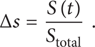
This delta distance will replace the free parameter t in the Hermite curve. By setting the increment of the time (dt), the delta distance for every dt will be

$\Delta s=\frac{s\left(\text{dt}\right)}{s_{\text{total}}}.$

(6)

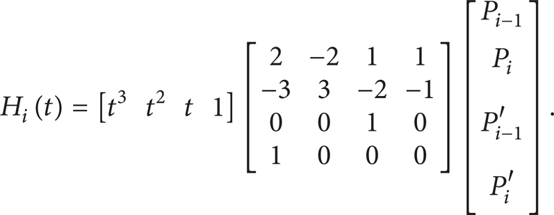
Therefore, the position of the vehicle at time dt can be calculated using (6), and ith piecewise Cubic Motion curve can be formed using

$H_i\left(\Delta s\right)=\left[\begin{array}{cccc}\Delta s^{\mathrm{3}}& \Delta s^{\mathrm{2}}& \Delta s& \mathrm{1}\end{array}\right]\left[\begin{array}{cccc}\mathrm{2}& -\mathrm{2}& \mathrm{1}& \mathrm{1}\\ -\mathrm{3}& \mathrm{3}& -\mathrm{2}& -\mathrm{1}\\ \mathrm{0}& \mathrm{0}& \mathrm{1}& \mathrm{0}\\ \mathrm{1}& \mathrm{0}& \mathrm{0}& \mathrm{0}\end{array}\right]\left[\begin{array}{c}{P}_{i-\mathrm{1}}\\ P_i\\ P_{i-\mathrm{1}}^{\prime }\\ P_i^{\prime }\end{array}\right],$

(7)

where H _i is the ith piecewise Cubic Motion curve, P_{i − 1} is the start control point, P _i is the end control point, P_{i − 1}′ is the tangent for start control point, and P _i ′ is the tangent for end control point.

The tangent of the start (P_{i − 1}′) and end (P _i ′) control points for each piecewise is solved using (1). When n numbers of curves are combined, Cubic Motion curve is generated.

2.1.3. Error Analysis

Error analysis is based on the length of the curve motion. For each delta time (dt), there will be a certain number of iterations required to calculate the total length of the curve. As dt becomes smaller, the number of iterations becomes larger. When the number of iterations and the total length of the curve are plotted, at a certain number of iterations, the length of the curve will not change with respect to the number of iterations, as shown in Figure 2. As the length of the curve is equal to the length of curve with previous dt, the system will terminate the iteration process and dt time will be used in the generation of the Cubic Motion curve.

Figure 2:

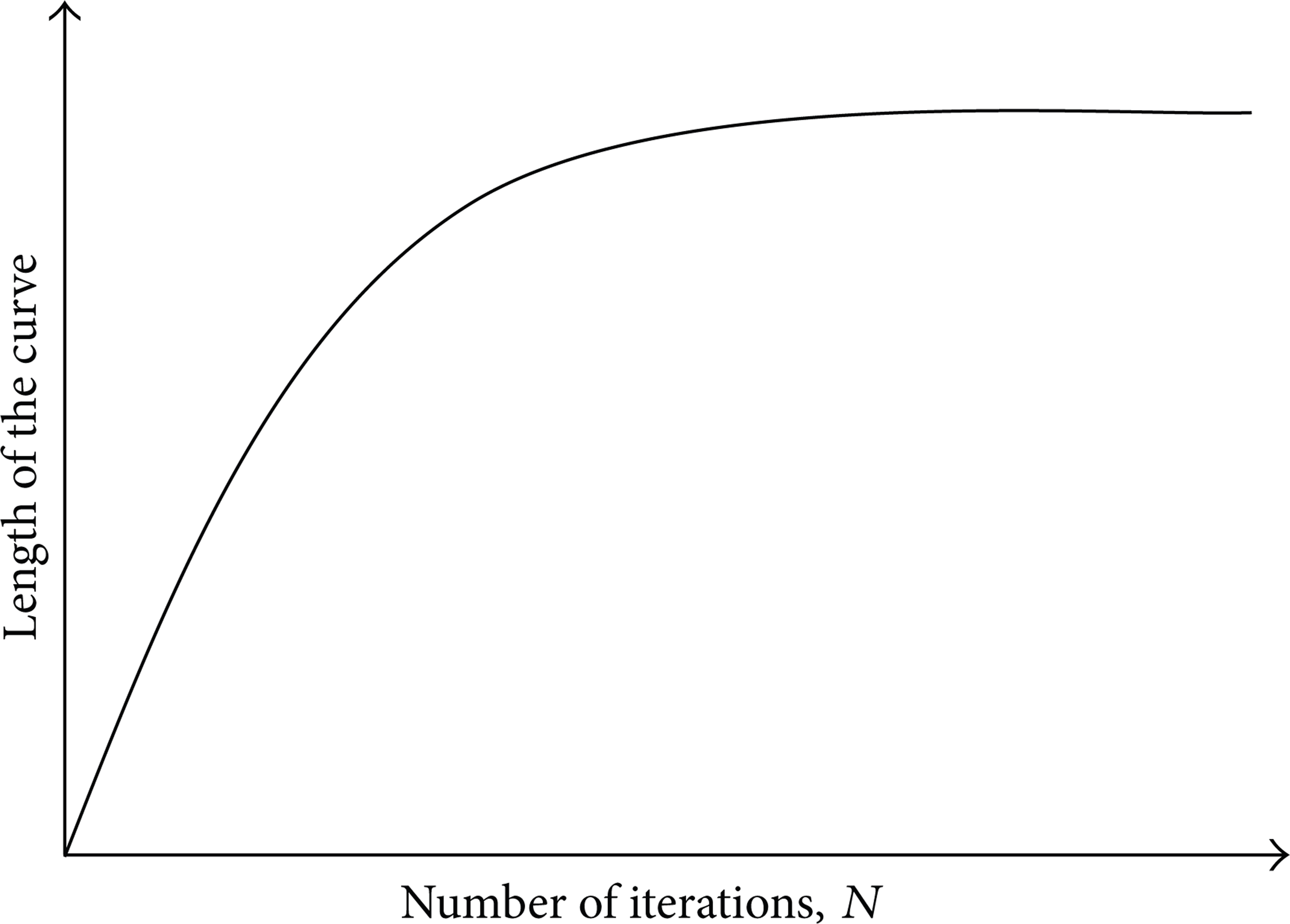
Number of iterations and length of the curve.

2.2. VDM-DM Module

Vehicle dynamic and driver models are the core of the module. The vehicle dynamic model (VDM) will calculate the dynamic response of the vehicle and the driver model will act as the driver to make the vehicle follow the intended path. In this system, the bicycle model [10] and Reński [11] are used for the VDM and the driver model, respectively.

The driver model will calculate the steer input based on the intended path. This steer input will then be used as the input VDM to calculate the trajectory. The y trajectory and yaw angle are then fed back to driver model to allow the driver to manoeuvre. This process is iteratively carried out and the outputs of the module are the trajectory from the driver model and dynamic vehicle response from the VDM.

2.2.1. Verification of the VDM-DM Module

The verification of the VDM model is done by comparing the body slip angle of Jazar's work [12] based on step input of the steer angle. The step input is shown in Figure 3, in which a sudden steer angle of 12° is applied. Figure 4(a) shows the body slip angle of Jazar's work. The result of the VDM model developed by this system is shown in Figure 4(b). Since the VDM model has shown similar results to Jazar's work, the VDM model has been verified.

Figure 3:

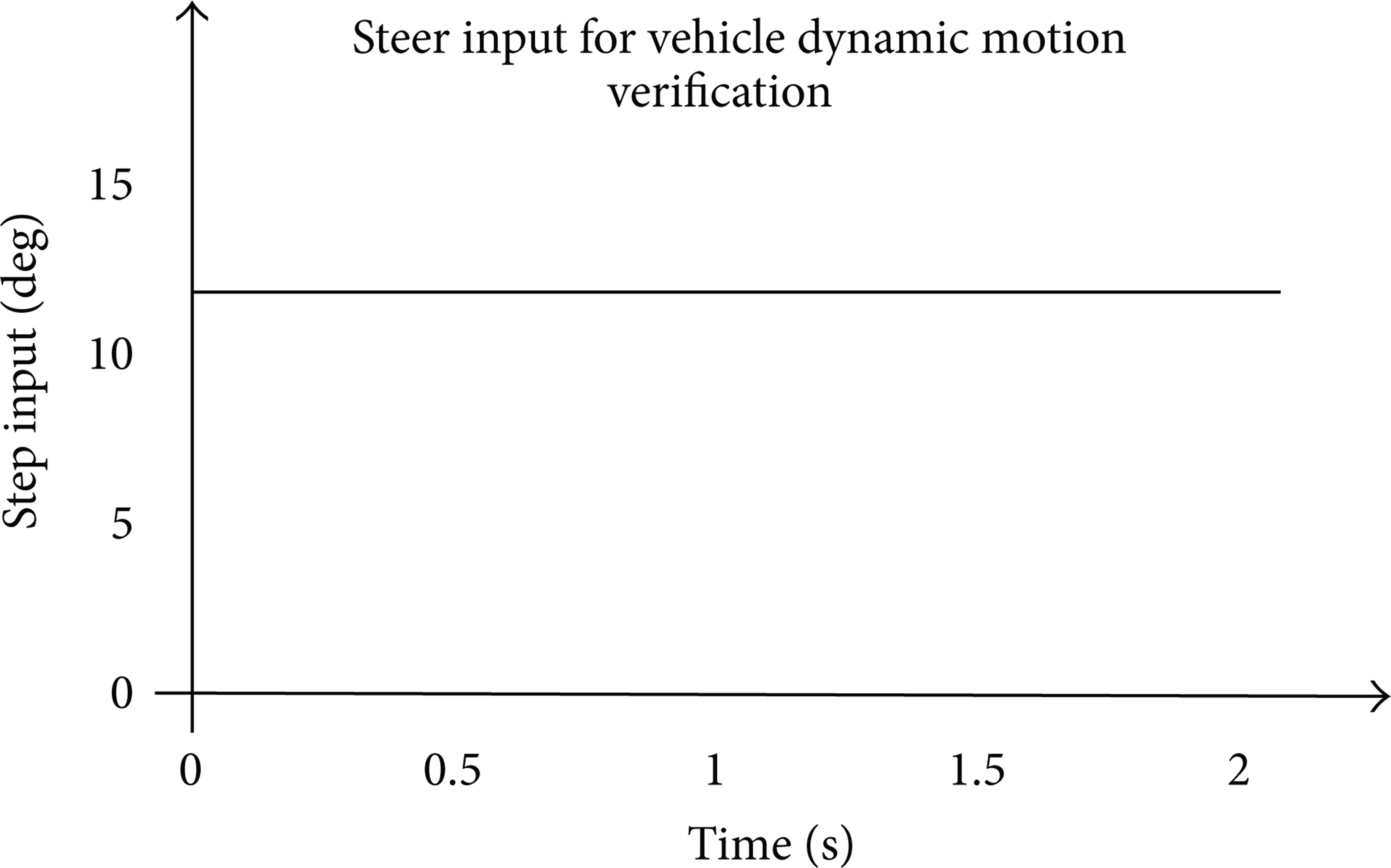
Step input of steer input.

Figure 4:

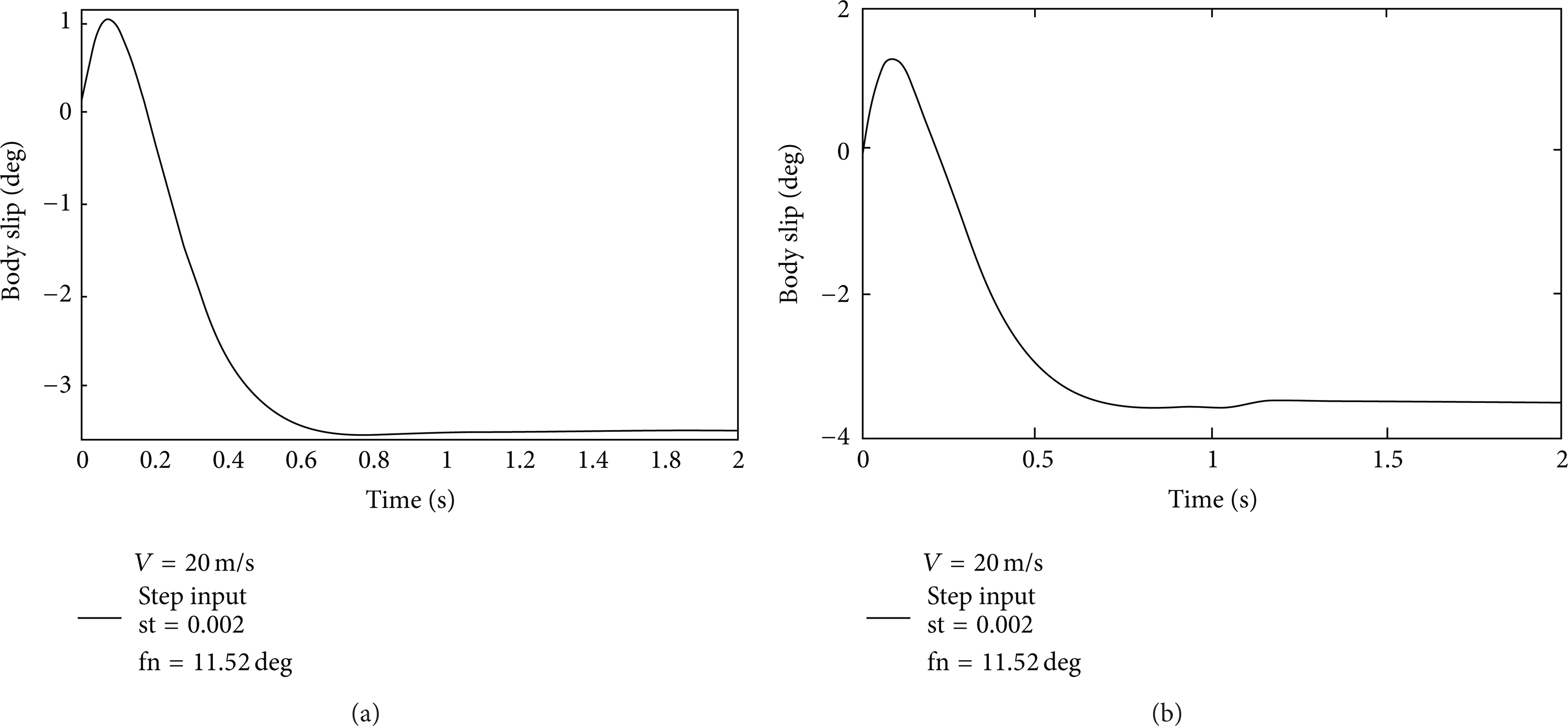
Vehicle response of (a) Jazar [12] and (b) the VDM module.

After the VDM has been verified, the next stage is to verify the driver model. The verification of the driver model is based on the result obtained, comparing it with the desired path. Ramp input as shown in Figure 5 is used as the input for the driver model. It is expected that the driver model will be able to steer the vehicle to follow the desired path.

Figure 5:

Ramp input for driver model.

The driver model is verified when it acts like a human. One of the important parameters of Andrzej Reński's driver model is sight length. The sight length is the horizontal length of the vehicle with respect to the destination point.

For the purpose of verification, the velocity is set as a constant at 20 km/h with various sight lengths. Figure 6 shows the trajectory of various sight lengths. As the sight length is reduced from 10 m, the deviation of the trajectory becomes smaller, and until the sight length is set to 1 m, the car is able to follow the bend route. Therefore, the driver model has been verified because it behaves as expected when the sight length becomes shorter; the manoeuvrability improves.

Figure 6:

Trajectory of various sight distances.

In fact, the sight length depends on the velocity of the vehicle. The faster the vehicle is, the longer the sight will be. In the case of the following case studies, the appropriate sight length is 3 m when the velocity of the vehicle is 40 km/h based on the observation of the deviation of the trajectory from the actual path.

2.3. Integrated Module

The final module will integrate the Cubic Motion module and the VDM-DM module. The Cubic Motion curve will provide the coordinates of vertices and velocity. Velocity can be retrieved from the distance between two vertices and delta time (dt) used. By additionally setting the sight length, the Cubic Motion curve can be used as the input to the VDM-DM module. Finally, steer input, trajectory and dynamic response of the car can be determined directly from Cubic Motion curve.

3. Case Studies

Two case studies are carried out, which are double lane change (DLC) and the Slalom test. Section 3.1 focuses on the generation of the three inputs for both case studies. Section 3.2 shows the results from the case studies. Finally, the discussion of the results will be in Section 4.

3.1. Cubic Motion Curve Input

This section will discuss the generation of three curves to be used as input for both case studies.

Double Lane Change (DLC). The DLC path is constructed using six control points (CP1 to CP6). Figure 7 shows the DLC path, and the six control points are CP1 (0, 0), CP2 (15, 0), CP3 (45, 3.5), CP4 (70, 3.5), CP5 (95,0), and CP6 (125, 0).

Figure 7:

DLC path.

Three types of Cubic Motion curves will be input into the system. Figure 8(a) shows the natural Cubic Motion curve. Due to the characteristics of the curve, deviation occurs at three locations, which are CP1-CP2, CP3-CP4, and CP5-CP6. However, the deviations are still within the road boundary, and thus it is acceptable to proceed with dynamic response analysis on the VDM-DM modules.

Figure 8:

Input: (a) natural Cubic Motion, (b) adjusted tangent Cubic Motion, and (c) additional vertices Cubic Motion.

To reduce the deviation, the tangent at the control points should be manually changed. Figure 8(b) shows the path generated when the tangents at each of the control points are set to 〈5, 0〉. Finally, control points are added before and after CP2, CP3, CP4, and CP5. Then, CP1 to CP5 are removed to make the sudden bend smoother when additional control points are added. This causes the total control points to become 10 points, as shown in Figure 8(c). The additional points are (7.5, 0) and (21, 0.5) replacing CP2, (40, 3) and (50, 3.5) replacing CP3, (65, 3.5) and (75, 3) replacing CP4, and (90, 0.5) and (100, 0) replacing CP5.

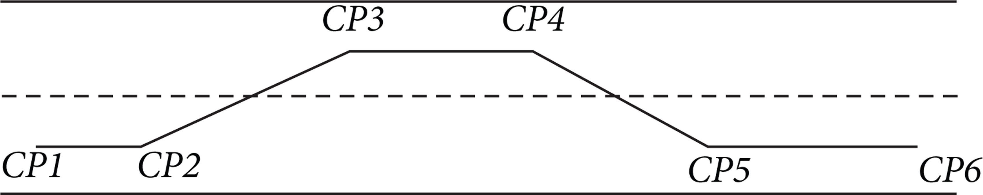
Slalom Test. The second case study is the Slalom test track. The aim of the test is to ensure that the vehicle is able to avoid the obstructions. This Slalom test track, as shown in Figure 9, is constructed according to six control points, which are CP1 (0, 0), CP2 (10, 0), CP3 (17.5, 3), CP4 (32.5, −3), CP5 (40, 0), and CP6 (50, 0). The distance between the obstructions is A = 15 m, while B = 3 m is the vertical distance of the obstructions and control points.

Figure 9:

Slalom test track.

The three types of input are shown in Figure 10. The natural Cubic Motion curve as shown in Figure 14(a) is generated based on the six control points. Similarly to the natural Cubic Motion for DLC case study, deviation from the path occurs from paths CP1-CP2 and CP5-CP6. Then, the tangents of CP1, CP2, CP5, and CP6 are set to be horizontal 〈5,0〉 and Cubic Motion, as shown in Figure 14(b), is generated. Lastly, to make the sudden sharp bend at CP2 and CP5, additional points are positioned at (7.5, 0) and (12, 1) replacing CP2 and at (37, −1) and (42.5, 0) replacing CP5. As a result, Cubic Motion will have eight control points, generated as shown in Figure 14(c).

Figure 10:

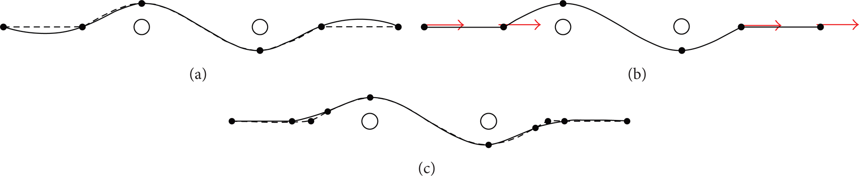
(a) Natural Cubic Motion curve, (b) adjusted tangent Cubic Motion, and (c) additional vertices Cubic Motion.

3.2. Trajectory, Steer Input, and Vehicle Responses

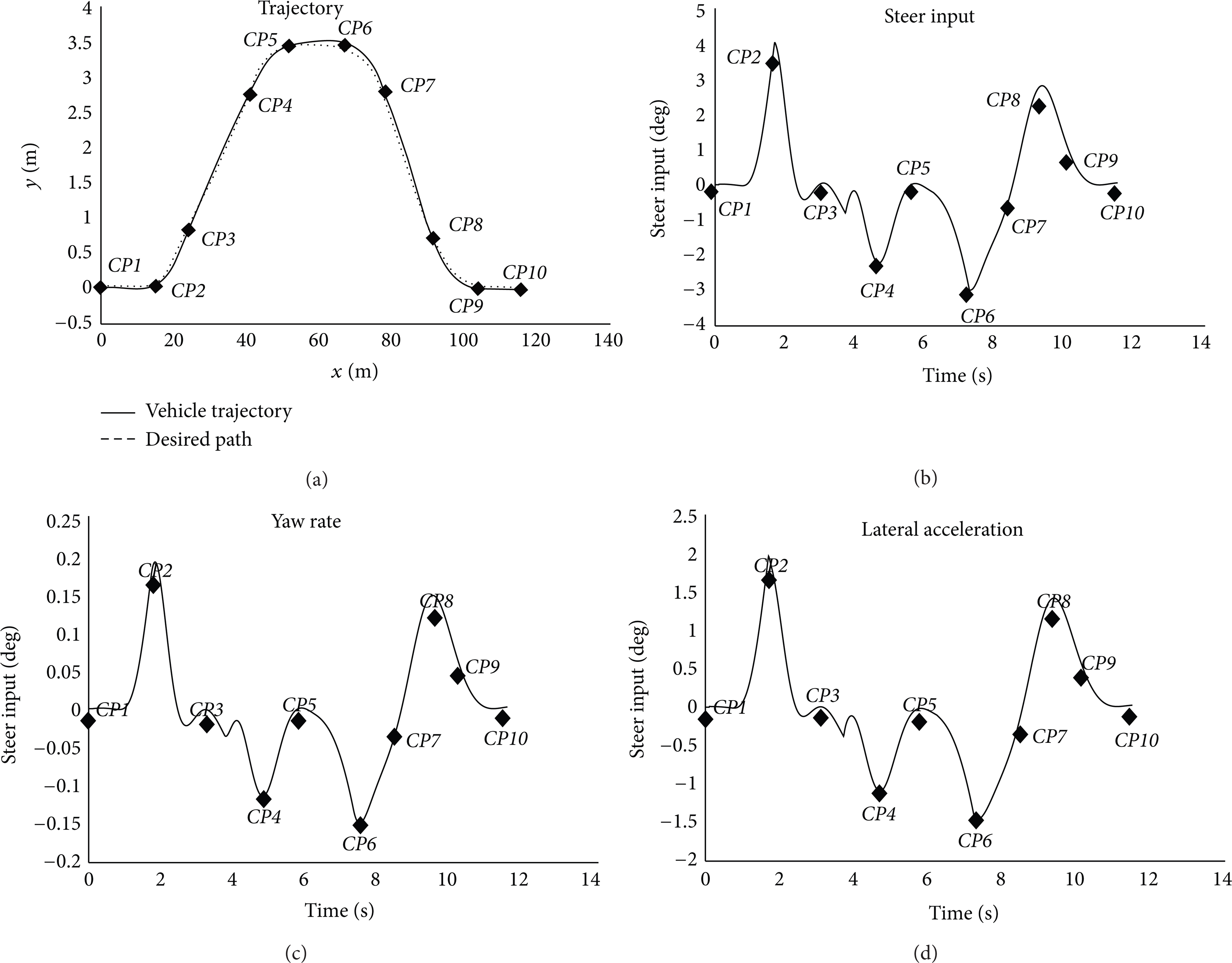
Results for each case study are described in this section. The results comprise trajectory, steer input, and vehicle response. The vehicle response includes yaw rate and lateral acceleration.

Double Lane Change (DLC). The first input is natural Cubic Motion. Due to the characteristics of natural Cubic Motion, the vehicle must turn to the left as it begins to move. Sudden left turning causes a sudden steer of −6° to be required. This sudden steer to the left causes a sudden change of yaw rate and lateral acceleration. As the vehicle turns to the left, the vehicle needs to turn to the right to go to CP2, and this again causes sudden changes in steer input, yaw rate, and lateral acceleration. Beyond CP2, no sudden change is detected in steer input and dynamic response. Figure 11 shows the trajectory, steer input, yaw rate, and lateral acceleration of the vehicle if natural Cubic Motion is used as the input.

Figure 11:

Results of natural Cubic Motion curve for DLC at velocity of 40 km/h.

The trajectory, steer input, and dynamic response of the vehicle based on adjusted tangent of the Cubic Motion curve are shown in Figure 12. The sudden change of direction at CP2, CP3, and CP4 demands a sudden change of steer input. At the same time, it causes sudden increments in the yaw rate and lateral acceleration of the vehicle.

Figure 12:

Results for adjusted tangent Cubic Motion curve for DLC at 40 km/h velocity.

The last input is an additional vertices Cubic Motion curve. The trajectory, steer input, and dynamic responses of the vehicle is shown in Figure 13. This smoother curve at the control points successfully reduces the required steer input at the control points. The reduction of the required steer input will eventually reduce the yaw rate and lateral acceleration.

Figure 13:

Results of additional vertices Cubic Motion curve for DLC at velocity 40 km/h.

Figure 14:

Results of the natural Cubic Motion for the Slalom test track at 40 km/h velocity.

Furthermore, additional information can be retrieved from the Cubic Motion curve; this information is useful for the study of motion. Table 1 shows additional information, specifically travelling time to complete the path and total distance traveled.

Table 1:

Additional information retrieval from each curve.

Curve type	Natural Cubic Motion	Adjusted tangent Cubic Motion	Additional vertices Cubic Motion
Maximum time	12.9 s	12.5 s	11.46 s
Total distance	125.55 m	125.47 m	120.39 m

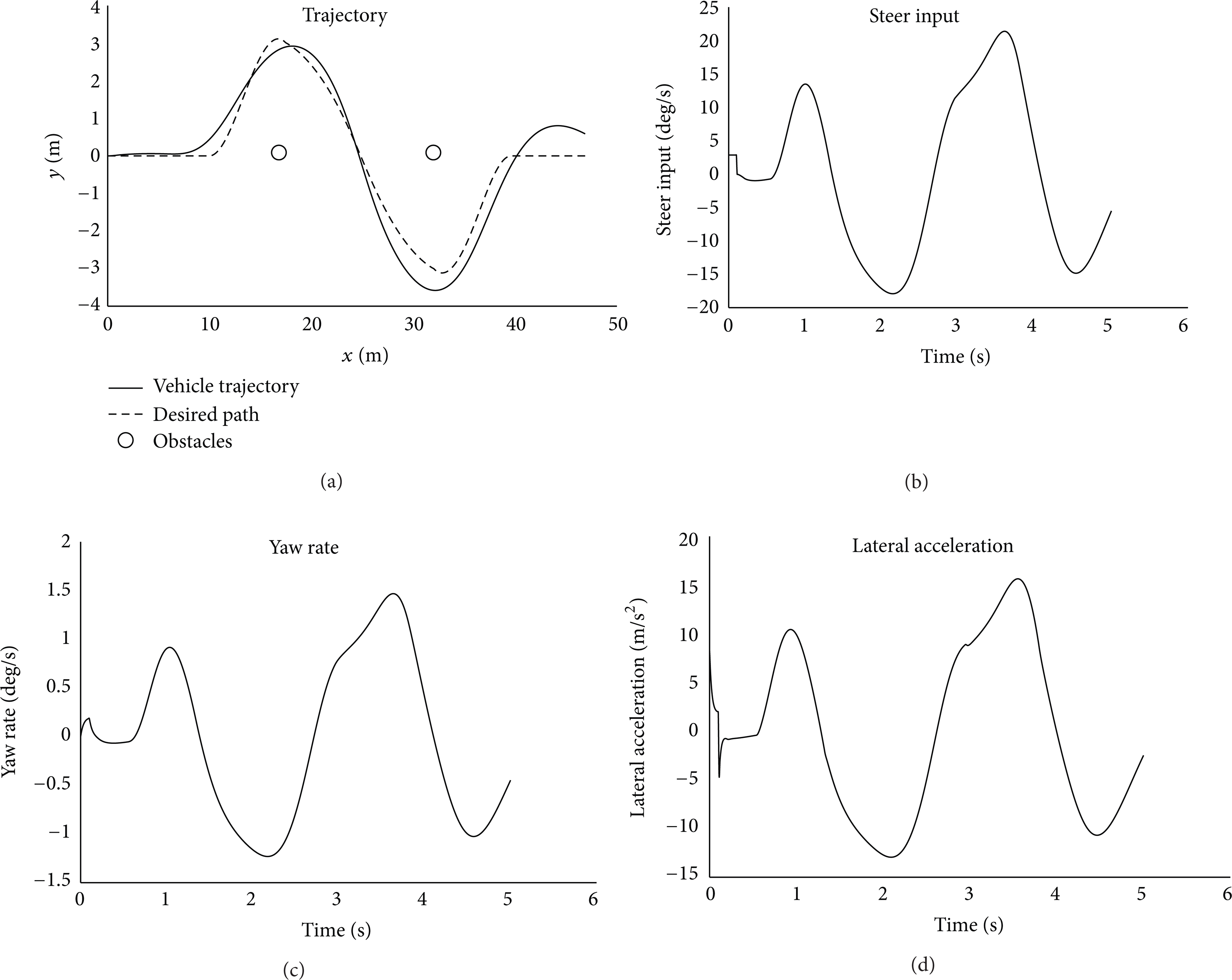
Slalom. In the case of the second case study, three types of input are again used with the intention of investigating whether these three inputs will yield similar results as the first case study. In the case of the input that is natural Cubic Motion, the sudden change of curve between CP1 and CP2 as the vehicle starts to move has little effect on the trajectory. Hence, it has little effect on the steer input, yaw rate, and lateral acceleration. Results of the natural Cubic Motion curve for the Slalom test track are shown in Figure 14.

The results of the adjusted tangent Cubic Motion curve as shown in Figure 15 are similar to the results of the additional vertices Cubic Motion curve as shown in Figure 16. This shows that the additional vertices to Cubic Motion have no effect on this curve.

Figure 15:

Results of adjusted tangent Cubic Motion for Slalom test track at velocity 40 km/h.

Figure 16:

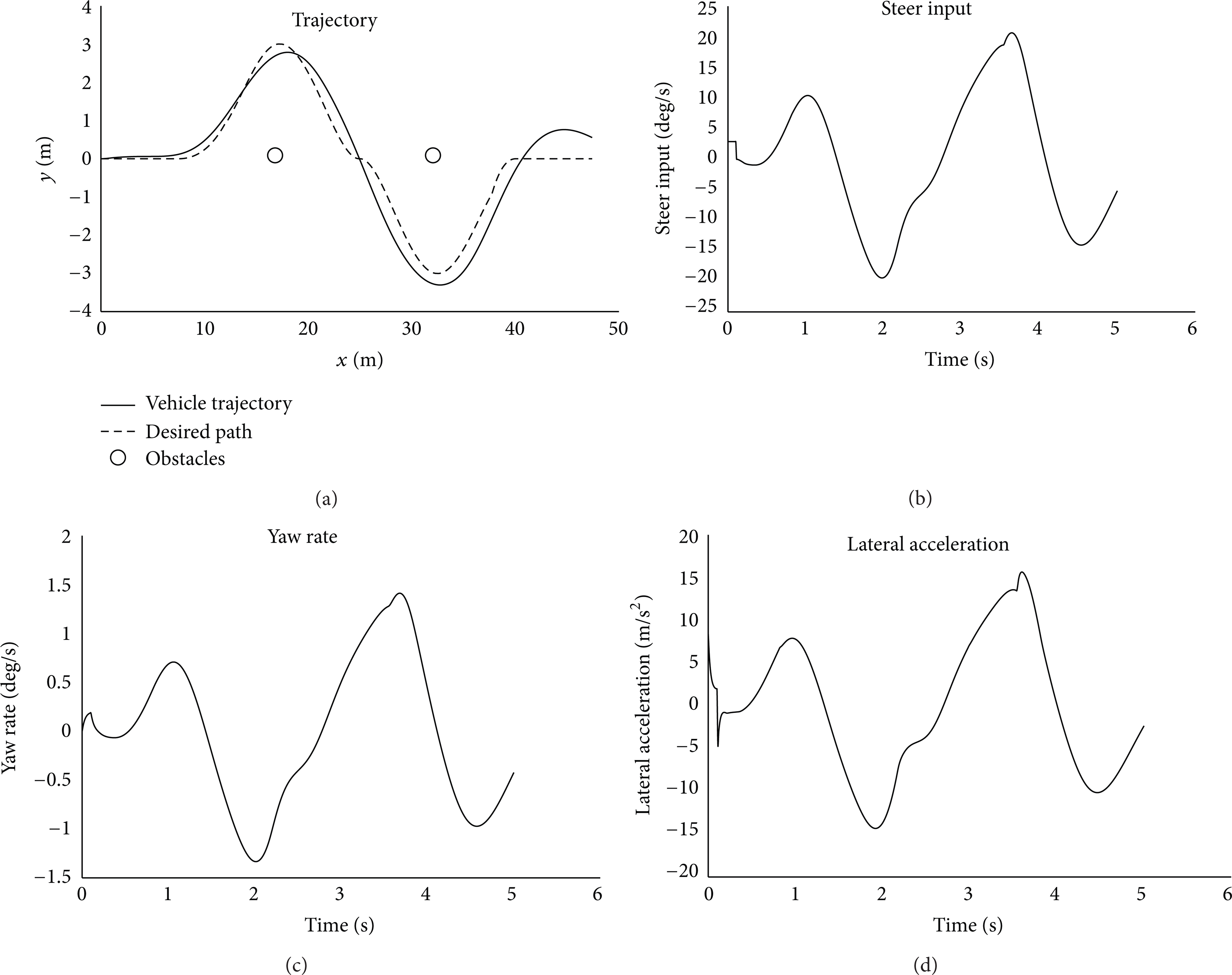
Results of additional vertices Cubic Motion for Slalom test track at velocity 40 km/h.

4. Discussion

Based on the two case studies, the three types of input can be used as the input to the VDM and driver model. The advantages of the implementation of Cubic Motion as the input are as described hereafter.

4.1. Compact Mathematical Representation

The mathematical representation of Cubic Motion requires three variables for each control point. The variables are coordinates, tangent, and the vehicle velocity of the control points. Moreover, the mathematical representation is generically applicable to linear and curvilinear motion.

4.2. Embedded Motion Attributes

The embedded motion attributes to the curve are in fact the nobility of the curve. The motion attributes can be retrieved directly from the curve for the vehicle dynamic and driver model calculation. This advantage becomes more distinct when the curve is made of a number of segments, in which all of the vertices on all of the segments will have equal time-based spacing.

4.3. Additional Information from the Curve

The input curve will have equal time-based spacing between two adjacent vertices and this will cause the trajectory produced to have equal time-based spacing. Based on the time-based equation, the total time taken to complete the whole trajectory can be retrieved from the curve together with the length of the path.

In fact, the final aim of the research is to bring road safety study to the desktop. When paths can be generated using Cubic Motion and can be directly transferred to this system, trajectory, steer input, and dynamic response can be predicted.

As this study is an exploratory study, the capability of the driver model has not been fully utilised. Delay of driver response in the driver model is set to one value. By further classifying the delay of driver response according to the classification of drivers, such as expert, normal, and novice, the trajectory of the vehicle can be predicted and finally the prediction of road accidents due to human or machine factor can be accomplished.

5. Conclusion

The main advantage of the Cubic Motion curve is the integration of path and motion in a single curve. This research has demonstrated that the curve itself is able to be used as the input for trajectory and dynamic response study. Therefore, the Cubic Motion curve is a compact representation of a curve that can be further explored in future research in the area of road safety.

Conflict of Interests

The authors declare that there is no conflict of interests regarding the publication of this paper.