Sage Journals: Discover world-class research

Abstract

Formation permeability distribution is important in the oil industry since it is a key tool in forecasting oil production performance, a matter of primary concern to oilfield operators. However, the direct problems of reservoir analysis are limited in practice by a lack of input parameters such as reservoir vertical heterogeneity. Therefore, inverse problem modeling is important to achieve reservoir vertical heterogeneity using production profiles, which are always known for existing reservoirs. In this way, what has occurred inside a reservoir can be understood by applying reservoir output in the reverse model. Because formation permeability can frequently be represented by a normal distribution and can describe heterogeneity and water production capability, an inverse problem of formation permeability was modeled to study reservoir vertical heterogeneity and reservoir production performance based on oil-water two-fluid flow theory and optimization problems. Moreover, through establishing an objective function, we obtained an optimal solution for water production rate. Finally, one case is simulated by this model and good results achieved, which are compatible with production and experimental data.

1. Introduction

In recent years, interesting research on formation permeability distribution and two-fluid flow modeling has been growing in conventional numerical reservoir simulation for the oil industry since it is a key to oil production performance, which in turn determines project profitability. In addition, the two-fluid model is used widely in other disciplines. For example, such modeling for particle-fluid fluidization is used in smoothed particle hydrodynamics [1], implementation of macroscale pseudoparticle modeling in gas-solid flow [2], and the study of large-scale direct numerical simulation (DNS) in gas-solid flows [3]. In reservoir analysis, a fast streamline-based computation method of sensitivity coefficients of fractional flow rate was studied based on inversion of dynamic production data in 2003 [4] and a method of subsurface inverse modeling was realized based on single-phase transient flow in 2011 [5]. Oil-water production can be simulated in the model as soon as the required parameters are defined in the forward two-phase model. However, it has been found that oil-water production is mostly governed by reservoir vertical heterogeneity, which is normally difficult to define [6, 7]. Therefore, inverse problem modeling must be done to achieve reservoir vertical heterogeneity using production profiles, which are always known for existing reservoirs. Thus, we can understand conditions inside a reservoir by applying reservoir output (e.g., oil-water production) in the reverse model. This provides a basis for estimating future production performance of a reservoir, which is very important to the reservoir operator.

At present, the study of the vertical permeability distribution is important for improving oil-driving efficiency and oil recovery. To investigate relevant problems in reservoir engineering, most studies rely on forward problems of seismic interpretation, logging interpretation, and core sampling experiments and combine these with mathematical statistics for a solution. As a result, many complex technologies and additional time will be needed [8 –10]. In addition, there is always a large error between calculation of the water production rate and historical rate in most reservoir water cut analysis [11, 12]. On the contrary, the process of the internal rules and exterior influence can be explored by the observed phenomenon and the result of the evolution, which can be called inverse problem process. Actually the studies of inverse problems have been spread over every field of the modern society in recent years such as oriented design, geophysical prospecting, and numerical simulation [13 –16].

Using the grid modeling method and optimization problems of water production rate, an inverse problem model was constructed based on formation permeability and two-phase flow. This facilitates not only research into the permeability distribution and injection profile, but also oil and water production analysis. This approach can provide a reference for heterogeneity by researching whether the vertical permeability distribution always obeys normal distribution. In Section 2.1, an objective function is established and optimal solution of water production rate is obtained, in order to reduce the error between the calculated production rates and historical water production rates in the inverse model. In Section 2.2, we infer the oil-water two-phase plane radial flow mathematical model and give a special definition of saturation called “frontier” saturation. Section 3 describes research into the inverse problem model of reservoir permeability when its logarithmic function obeys a normal distribution, and related theories and methods are introduced. Section 4 provides definitions and establishes the steps of productivity analysis for the fluid-producing edge in the reservoir grid model. A case study is used for reservoir analysis in Section 5, and conclusions are drawn in Section 6. Finally, an inverse problem model between water production rate and heterogeneity was established, which not only can calculate water and oil production but also can show the physical phenomenon of injection profile.

2. Mathematical Models of Oil-Water Two-Phase Plane Radial Flow

2.1. Reservoir Profile Model

As shown in Figure 1, a reservoir profile grid model was established for describing relevant physical processes. This is the model supporting our research.

Figure 1:

Reservoir profile grid model.

The research model focuses on a minimum-differential problem between calculated and historical water production rates, to investigate the inverse problem mathematical model and optimization problems of water production and formation permeability distribution. The problem can be reformulated as the following optimization problem:

\begin{matrix} \begin{matrix} \min_{f_{w} (x), y} & E = | f_{w} (x) - y | \end{matrix} \\ \begin{matrix} s . t . & f_{w} (x) = \frac{W (x)}{W (x) + O (x)} \end{matrix} \\ \begin{matrix} W (x) + O (x) > 0 \end{matrix} \\ \begin{matrix} W (x) \geq 0, O (x) \geq 0, x \geq 0, y \geq 0 . \end{matrix} \end{matrix}

(1)

The mathematical model for researching the water saturation x in the fluid-producing edge is as follows:

x = {\begin{cases} S_{0}, & r e > r w f \\ G (F_{w} (x)), & r e \leq r w f, \end{cases}

(2)

where G is a functional relation of water saturation which can be obtained from a set of experimental data S_w and F_w(S_w), which can be denoted by other experimental data between ΔS_w and Δf_w when re ≤ rwf.

Actually, we can describe water production rate at different times based on a specified time step for a more convenient study of reservoir production. Therefore, the above problem can be done in a simplified consideration. In vector space Cⁿ(Rⁿ), we can obtain $[f_{w 1}, f_{w 2}, \dots, f_{w n}] \in C^{n}$ and $[x_{1}, x_{2}, \dots, x_{n}] \in C^{n}$ , y is denoted as $[y_{1}, y_{2}, \dots, y_{n}] \in C^{n}$ , and the previous expressions can be equivalent to another problem as the following optimization problem at different time steps. At this point, n is the total number of time steps. Consider

\min_{f_{w i}, y_{i}} E = \sum_{i = 1}^{n t} {({f_{w}}_{i} - y_{i})}^{2} .

(3)

The model will contain the Buckley-Leverett theory of two-phase flow and establishes the oil-water two-phase plane radial flow function [17] for establishing an inverse problem model of reservoir permeability in each longitudinal grid layer, and the model will also show the displacement of frontier saturation and solution of the water production rate.

2.2. Derivation of Oil-Water Two-Phase Theory Based on Plane Radial Flow

Using the Buckley-Leverett theory of two-phase flow, without considering factors of gravity and capillary pressure, we established the oil-water two-phase plane radial flow mathematical model $r e^{2} - r^{2} = ((F_{w} (S_{w}) \cdot Q) / ϕ \cdot π \cdot h)$ .

We suppose the liquid flow rule is a plane radial flow from reservoir limit to well and choose a volume unit in the streamline vertical direction, as shown in Figure 2.

Figure 2:

Plane radial flow model unit.

Relying on the seepage principle [18], we have the flow equation:

q_{w} = q \cdot f_{w} .

(4)

The flow volume of the volume element in dt time is

Q_{out} = d q_{w} \cdot d t .

(5)

From (4) and (5) we obtain

Q_{out} = q \cdot d f_{w} \cdot d t .

(6)

Inflow volume of the volume element is

Q_{in} = ϕ \cdot 2 π h \cdot r d r \cdot d s_{w} .

(7)

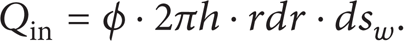
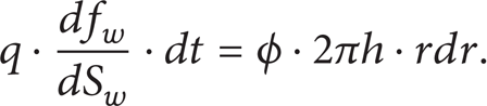
According to the Buckley-Leverett theory for oil-water two-phase flow in time Δt:Q_in = Q_out.

From (6) and (7), we have q·df_w·dt = ϕ·2πh·rdr·dS_w, as follows:

q \cdot \frac{d f_{w}}{d S_{w}} \cdot d t = ϕ \cdot 2 π h \cdot r d r .

(8)

Defining $F_{w} (S_{w}) = (d f_{w} / d S_{w})$ and deriving from (8), we have

F_{w} (S_{w}) \cdot q (t) \cdot d t = ϕ \cdot 2 π h \cdot r d r .

(9)

We obtain $F_{w} (S_{w}) = (d f_{w} / d S_{w})$ from f_w = f_w(S_w) with rules for taking derivatives, derived from (8) and q·F_w(S_w)·dt = ϕ·2πh·rdr. After infinitesimal calculus, we obtain

F_{w} (S_{w}) \cdot \int_{0}^{t} q d t = ϕ \cdot 2 π h \cdot \int_{r}^{r e} r d r .

(10)

Because of $Q (t) = \int_{0}^{t} q \cdot d t$ , (10) becomes F_w·Q = ϕ·πh·(re²-r²) and we have

r e^{2} - r^{2} = \frac{F_{w} (S_{w}) \cdot Q (t)}{ϕ \cdot π h} .

(11)

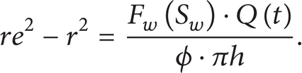
For the reservoir profile grid model, the plane radial flow model of the grids in each longitudinal layer yields

r e^{2} - r_{i, j}^{2} = \frac{F_{w} (S_{w_{i, j}}) Q_{j}}{ϕ_{j} \cdot π h_{j}} .

(12)

A special definition of saturation “S_wf”: from the water cut function curve f_w = f_w(S_wf) and selecting the point of irreducible water saturation as a fixed point and joining any other point on the curve, with constructing function $k (S_{w} f) = (f_{w} (S_{w} f) - f_{w} (S_{w_{1}})) / (S_{w} f - S_{w_{1}})$ and if and only if $Max {k (S_{w} f)}$ can be found, we call S_wf the frontier saturation. Therefore, we obtain the corresponding displacement of frontier saturation rwf for each layer, as shown by the following equation and Figure 3:

r w f_{j}^{2} = r e^{2} - \frac{F_{w} (S_{w} f_{i, j}) Q_{j}}{ϕ_{j} \cdot π h_{j}} .

(13)

Figure 3:

Frontier saturation diagram.

We can calculate the front position of water driving in each grid layer at different times from (13).

3. Research on Whether the Inverse Problem Model of Formation Permeability Logarithmic Function Always Obeys Normal Distribution

If the formation permeability logarithmic function distribution ${\log K_{1}, \log K_{2}, \dots, \log K_{n}}$ always obeys a normal distribution of $μ = \log \bar{K}$ , then we calculate the value of f_w(x) based on (11), which can be adapted to objective function (1). Finally, it will give the optimal result of water production rate or the optimal distributions ${\log K_{1}, \log K_{2}, \dots, \log K_{n}}$ and ${K_{1}, K_{2}, \dots, K_{n}}$ .

According to the 3σ principle, or a normal distribution curve, if P (μ-3σ-a<X ≤ μ + 3σ + a) = 1, there are left and right endpoints on the curve. The left endpoint is log⁡K_min or μ-3σ-a on the X-axis, and the right endpoint is log⁡K_max or μ + 3σ + a on that axis, and so forth: a>0 ( $μ = \log \bar{K} = 0.5 \cdot (\log K_{\min} + \log K_{\max})$ ).

According to the area superposition principle of a normal distribution curve [19]: selecting $x = \log \bar{K}$ as the starting point and step size Δx, subdivide the probability curve. If area summation of these form-closed figures can infinitely approach 1, we can obtain the values of the left endpoint log⁡K_min and right endpoint log⁡K_max and so forth; $\log K_{\max} = 2 \cdot \log \bar{K} - \log K_{\min}$ . See Figure 4.

Figure 4:

Area-dividing distribution function with equal steps.

By the area superposition principle of the normal distribution and establishing an initial value σ of that distribution, and so forth, X₀ = log⁡K_min, X_n = log⁡K_max, p = n + 1. F(X_j) is a cumulative distribution function of the normal distribution [20]. Using equal step size ΔX to subdivide the probability curve, the area summation of every closed figure S_j = F(X_j)-F(X_j–1), X_j = ΔX·j + X₀, K_j = exp⁡(X_j) and longitudinal strata thickness of each layer h_j = h·S_j. If we use equal area ΔS to subdivide for probability curve, the area summation of every closed figure is S_j = F(X_j)-F(X_j–1), $S_{j} = Δ S = (1 / n)$ , h_j = h·S_j, and X_j = F⁻¹(S_j), K_j = exp⁡(X_j), and so forth, j = 1,2,3,…, n (n is the total number of vertical stratifications).

Relying on the distribution ${K_{1}, K_{2}, \dots, K_{n}}$ and the oil-water relative permeability functions [21]: kro_i,j = kro (S_{w
_i,j}) and krw_i,j = krw (S_{w
_i,j}), for each grid and conductivity definition [22 –25], we can calculate the conductivity equation for all grids as follows:

T = \frac{2 π h_{j} K_{j}}{\log (r e / r_{i, j})} (\frac{K r o_{i, j}}{μ_{o}} + \frac{K r w_{i, j}}{μ_{w}}) .

(14)

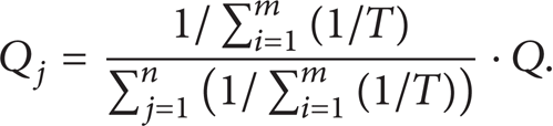
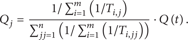
We can differentiate production and calculate liquid production Q_j in each layer at different times according to

Q_{j} = \frac{1 / \sum_{i = 1}^{m} (1 / T)}{\sum_{j = 1}^{n} (1 / \sum_{i = 1}^{m} (1 / T))} \cdot Q .

(15)

We obtain the front position of water driving rwf_j as derived from (13) and (15).

When re ≤ rwf_j and solving the inverse function of (12) and calculating water saturation of the fluid-producing edge, then S_w = G(F_w(S_w)), and so forth, i = 1. If re>rwf_j, then S_{w
_i,j} = S₀, and so forth, i = 1.

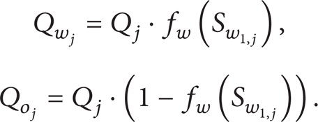
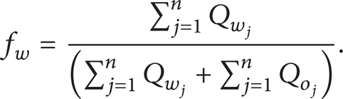
When we have the water saturation (S_w) [26] of each layer, relying on the function f_w = f_w(S_w), the water cut for longitudinal each layer f_w(S_{w
_1,j}) is calculated. Ultimately, oil production Q_{o
_j} and water production Q_{w
_j} are obtained. The corresponding mathematical model is

\begin{matrix} Q_{w_{j}} = Q_{j} \cdot f_{w} (S_{w_{1, j}}), \\ Q_{o_{j}} = Q_{j} \cdot (1 - f_{w} (S_{w_{1, j}})) . \end{matrix}

(16)

When we obtain the oil and water production in each layer, the total water production rate can be calculated at the fluid-producing edge according to

f_{w} = \frac{\sum_{j = 1}^{n} Q_{w_{j}}}{(\sum_{j = 1}^{n} Q_{w_{j}} + \sum_{j = 1}^{n} Q_{o_{j}})} .

(17)

Relying on the results of (17) and the objective function (1) as a determinant of the optimization problem, the optimal calculation water production rate f_w is found at different times. The standard deviation σ and distributions ${\log K_{1}, \log K_{2}, \dots, \log K_{n}}$ and ${K_{1}, K_{2}, \dots, K_{n}}$ are obtained by the numerical optimization calculation in the inverse problem model.

4. Fluid-Producing Edge Productivity Analysis for Reservoir Profile Model

4.1. Parameter Definitions

Water saturation of grid (S_{w
_i,j}): the center of each grid corresponds to water saturation.

Water saturation of the fluid-producing edge (x = S_{w
_1,j}): the water saturation of the grid is next to the fluid-producing edge in each layer.

Water production rate of grid (f_w(S_{w
_i,j})): the center of each grid corresponds to the water production rate.

Water production rate of the fluid-producing edge (f_w(S_{w
_1,j})): the water cut of the grid is next to the fluid-producing edge in each layer.

4.2. Productivity Analysis for Fluid-Producing Edge

To calculate the water cut of the fluid-producing edge at different times, we can use the following steps.

Step 1. Counting total fluid production of each vertical layer at different times,

Q_{j} = \frac{1 / \sum_{i = 1}^{m} (1 / T_{i, j})}{\sum_{j j = 1}^{n} (1 / \sum_{i = 1}^{m} (1 / T_{i, j j}))} \cdot Q (t) .

(18)

Step 2. In each grid layer, we obtain the derivative of water production rate in the fluid-producing edge from (13), when re ≤ rwf_j

F_{w} (x) = \frac{(r e^{2} - r_{1, j}^{2}) \cdot ϕ_{j} \cdot π \cdot h_{j}}{Q_{j}} .

(19)

Step 3. Solving a functional relation between S and F_w: x = S_{w
_1,j} = G(F_w(x)), we obtain the value of S_{w
_1,j} (S_{w
_1,j} = S₀ when re>rwf_j).

Step 4. Relying on S_{w
_1,j} and the functional relation f_w = f_w(S_w), we obtain the value of f_w(x)_j in each grid layer.

Step 5. When we have the value of f_w(x)_j, oil and water production can be calculated in each grid layer from the following:

\begin{array}{l} O {(x)}_{j} = Q {(x)}_{j} \cdot (1 - f_{w} {(x)}_{j}), \\ W {(x)}_{j} = Q {(x)}_{j} \cdot f_{w} {(x)}_{j} . \end{array}

(20)

Step 6. Total oil-water production and total calculated water production rate of the fluid-producing edge can be calculated as follows:

\begin{array}{l} O (x) = \sum_{j = 1}^{n} O {(x)}_{j}, \\ W (x) = \sum_{j = 1}^{n} W {(x)}_{j}, \\ f_{w} (x) = \frac{W (x)}{W (x) + O (x)} . \end{array}

(21)

Step 7. Find the optimal solution of water production rate and put all results of the calculated water production rate into the objective function (1) in the inverse mathematical model. If the result of water production rate does not meet corresponding requirements, modify the parameters as required and repeat the above steps until the optimal solution of that rate is obtained.

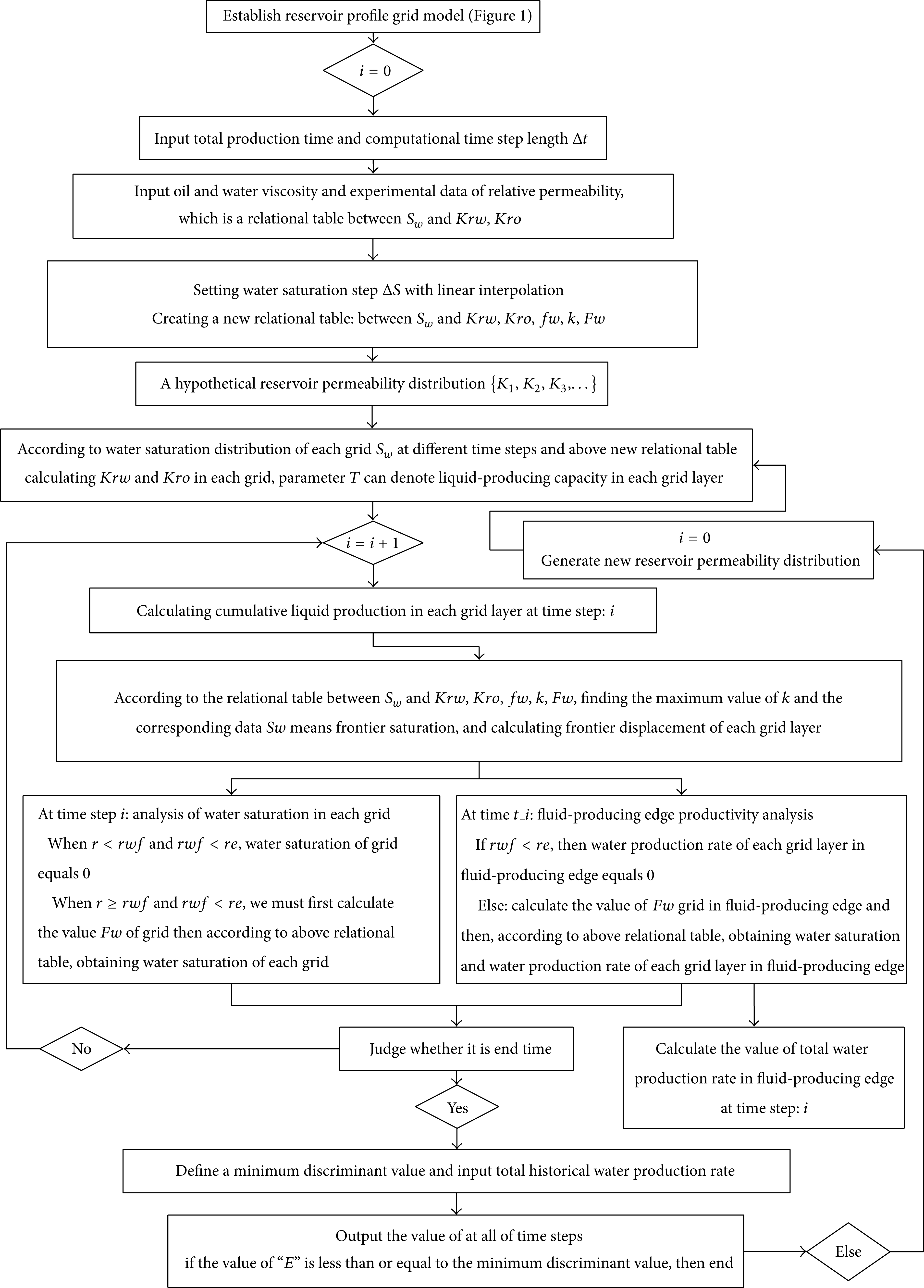
4.3. The Flow Diagram for Calculating Water Production Rate

See Figure 8.

5. Example Application for Reservoir Analysis

5.1. A Set of Reservoir Physical Property Data and Production Data

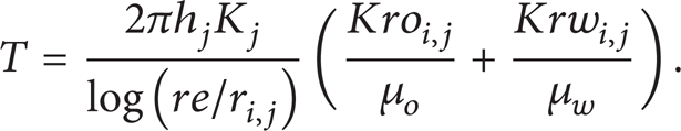
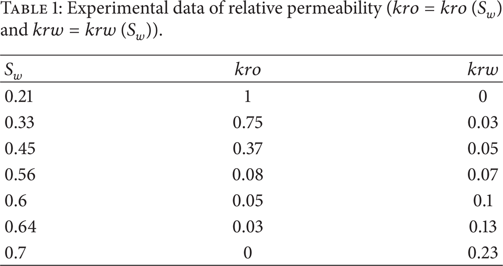
Reservoir Data. Reservoir radius re = 150 m; oil viscosity μ_o = 2.4 mpa·s; water viscosity μ_w = 0.9 mpa·s; reservoir thickness h = 50 m; average permeability $\bar{K} = 27 mD$ original water saturation S₀ = 0.21. See Tables 1 and 2.

Table 1:

Experimental data of relative permeability (kro = kro (S_w) and krw = krw (S_w)).

S _w	kro	krw

0.21	1	0
0.33	0.75	0.03
0.45	0.37	0.05
0.56	0.08	0.07
0.6	0.05	0.1
0.64	0.03	0.13
0.7	0	0.23

Table 2:

Geologic description.

TVD (m)	ϕ	K (mD)

1869	0.2	9
1878	0.2	40
1883	0.25	30
1891	0.197	40
1900	0.2	12
1919	0.19	10

Production data:

total computing time Time = 4000 d.

Production Data. Total computing time Time = 4000 d.

In the reservoir profile grid model based on Figure 1, time steps ΔT = 60 d; average partition total m = 20; partition total n = 20. See Tables 3 and 4.

Table 3:

Average liquid production data of reservoir.

Time (d)	q (m³/d)

0	300
2000	2802
3000	250

Table 4:

Total historical water production rate.

Time (d)	0	400	800	1200	1600	2000	2400	3000	3500	4000

y	0	0.025	0.095	0.252	0.376	0.522	0.585	0.665	0.7	0.708

5.2. Results

The front position of water driving based on the reservoir profile grid model at different times is shown in Figures 5 and 6 (blue indicates water; the border of blue and red is the front position of water driving in each grid layer).

Figure 5:

Front position of water driving (180 days).

Figure 6:

Front position of water driving (3000 days).

Relying on the objective function (1), we can obtain the calculated water production rate versus the historical rate, which can provide a basis for calculation (Figure 7).

Figure 7:

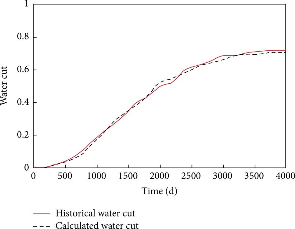
Comparison of water production rate.

Figure 8:

According to above results, we can learn that a good history matching effect of water production rate can be obtained from a set of suitable permeability distribution and other relevant data.

6. Conclusions

Relying on the above inverse problem model and the definition of normal distribution, we expect that the different variance distributions will correspond to their own normal distributions. If the standard deviation increases, the volatility of its normal distribution will be greater per the definition of standard deviation. This will lead to different permeability distributions, and the distribution curve can describe heterogeneity. The approach also determines liquid production, water production, and the integrated water production rate of the entire liquid outlet of each individual formation. Combined with the objective function, this produces a set of optimum normal distributions via the optimization solution method.

Finally, oil production and water production rates can be determined in the inverse problem model by analysis of changes of water driving location. The goal of constructing an inverse problem mathematical model according to historical dynamic production data can be realized. This permits the study of reservoir heterogeneity, prediction of dynamic production performance, and observation of the water flooding front position.

Footnotes

Nomenclature

Conflict of Interests

The authors declare that there is no conflict of interests regarding the publication of this paper.

Acknowledgments

The authors gratefully thank the referees for their valuable suggestions and the support of Canada CMG Foundation.

References

Xiong

Deng

Wang

, and Ge

, “SPH method for two-fluid modeling of particle-fluid fluidization,” Chemical Engineering Science, vol. 66, no. 9, pp. 1859–1865, 2011.

Xiong

Chen

, and Li

, “Direct numerical simulation of sub-grid structures in gas-solid flow-GPU implementation of macro-scale pseudo-particle modeling,” Chemical Engineering Science, vol. 65, no. 19, pp. 5356–5365, 2010.

Xiong

Zhou

, “Large-scale DNS of gas-solid flows on Mole-8.5,” Chemical Engineering Science, vol. 71, pp. 422–430, 2012.

Wen

X.-H.

Deutsch

C. V.

, and Cullick

A. S.

, “Inversion of dynamic production data for permeability: fast streamline-based computation of sensitivity coefficients of fractional flow rate,” Journal of Hydrology, vol. 281, no. 4, pp. 296–312, 2003.

Caers

, and Tchelepi

H. A.

, “A multiscale method for subsurface inverse modeling: single-phase transient flow,” Advances in Water Resources, vol. 34, no. 8, pp. 967–979, 2011.

Rezaee

Rostami

, and Pourafshary

, “Heterogeneity effect on non-wetting phase trapping in strong water drive gas reservoirs,” Journal of Natural Gas Science and Engineering, vol. 14, pp. 185–191, 2013.

Luo

R.-N.

, and Jiang

P.-X.

, “Numerical investigation of the influence of vertical permeability heterogeneity in stratified formation and of injection/production well perforation placement on CO2 geological storage with enhanced CH4 recovery,” Applied Energy, vol. 102, pp. 1314–1323, 2013.

Qin

Wang

G. G. X.

, and Rudolph

, “Evaluation of coal structure and permeability with the aid of geophysical logging technology,” Fuel, vol. 88, no. 11, pp. 2278–2285, 2009.

Leah

B. C.

Daniel

, and Soumyajit

, “Chirped CPMG for well-logging NMR applications,” Journal of Magnetic Resonance, vol. 242, pp. 197–202, 2014.

10.

Liu

Yao

Cai

, and Qiu

, “Evaluation of the reservoir permeability of anthracite coals by geophysical logging data,” International Journal of Coal Geology, vol. 87, no. 2, pp. 121–127, 2011.

11.

Dakuang

, “On concepts, strategies and techniques to the secondary development of China's high water-cut oilfields,” Petroleum Exploration and Development, vol. 37, no. 5, pp. 583–591, 2010.

12.

Vazquez

Mackay

, and Sorbie

, “A two-phase near-wellbore simulator to model non-aqueous scale inhibitor squeeze treatments,” Journal of Petroleum Science and Engineering, vol. 82–83, pp. 90–99, 2012.

13.

Xin

Han

Feng

, and Feng

, “Inverse design of an organ-oriented RF coil for open, vertical-field, MR-guided, focused ultrasound surgery,” Finite Elements in Analysis and Design, vol. 30, pp. 1519–1526, 2012.

14.

Takewaki

, “Incremental inverse eigenmode problem for performance-based structural redesign,” Finite Elements in Analysis and Design, vol. 27, no. 2, pp. 175–191, 1997.

15.

Alekseev

A. S.

and Mikhailenko

B. G.

, “Mathematical models of elastic wave processes in seismology and seismic prospecting: forward and inverse problems,” Simulation Practice and Theory, vol. 7, no. 2, pp. 125–151, 1999.

16.

Goncharsky

A. V.

Romanov

S. Y.

, and Seryozhnikov

S. Y.

, “Inverse problems of 3D ultrasonic tomography with complete and incomplete range data,” Wave Motion, vol. 51, pp. 389–404, 2014.

17.

Doster

and Hilfer

, “Generalized Buckley-Leverett theory for two-phase flow in porous media,” New Journal of Physics, vol. 13, Article ID 123030, 2011.

18.

Dibenedetto

Gianazza

, and Vespri

, “Continuity of the saturation in the flow of two immiscible fluids in a porous medium,” Indiana University Mathematics Journal, vol. 59, no. 6, pp. 2041–2076, 2010.

19.

Lévy

and Maïda

, “Central limit theorem for the heat kernel measure on the unitary group,” Journal of Functional Analysis, vol. 259, no. 12, pp. 3163–3204, 2010.

20.

Bonnéry

Breidt

F. J.

, and Coquet

, “Uniform convergence of the empirical cumulative distribution function under informative selection from a finite population,” Bernoulli, vol. 18, no. 4, pp. 1361–1385, 2012.

21.

Ramstad

Idowu

Nardi

, and Øren

P.-E.

, “Relative permeability calculations from two-phase flow simulations directly on digital images of porous rocks,” Transport in Porous Media, vol. 94, no. 2, pp. 487–504, 2012.

22.

Bing

S. X.

, “Reservoir numerical simulation study based on formation parameters' time-variability,” Procedia Engineering, vol. 29, pp. 2327–2331, 2012.

23.

Dumkwu

F. A.

Islam

A. W.

, and Carlson

E. S.

, “Review of well models and assessment of their impacts on numerical reservoir simulation performance,” Journal of Petroleum Science and Engineering, vol. 82–83, pp. 174–186, 2012.

24.

Liu

Yang

, and Wang

, “The model and algorithm of a new numerical simulation software for low permeability reservoirs,” Journal of Petroleum Science and Engineering, vol. 78, no. 2, pp. 239–242, 2011.

25.

Fassihi

M. R.

, “Treatment of transmissibilities when modelling symmetry elements,” Journal of Petroleum Science and Engineering, vol. 9, no. 4, pp. 267–271, 1993.

26.

Brailovsky

Babchin

Frankel

, and Sivashinsky

, “Fingering instability in water-oil displacement,” Transport in Porous Media, vol. 63, no. 3, pp. 363–380, 2006.

An Estimation Method of Water Drive Displacement Based on Formation Permeability Distribution and Inverse Problem Modeling

Abstract

1. Introduction

2. Mathematical Models of Oil-Water Two-Phase Plane Radial Flow

2.1. Reservoir Profile Model

2.2. Derivation of Oil-Water Two-Phase Theory Based on Plane Radial Flow

3. Research on Whether the Inverse Problem Model of Formation Permeability Logarithmic Function Always Obeys Normal Distribution

4. Fluid-Producing Edge Productivity Analysis for Reservoir Profile Model

4.1. Parameter Definitions

4.2. Productivity Analysis for Fluid-Producing Edge

4.3. The Flow Diagram for Calculating Water Production Rate

5. Example Application for Reservoir Analysis

5.1. A Set of Reservoir Physical Property Data and Production Data

5.2. Results

6. Conclusions

Footnotes

Nomenclature

Conflict of Interests

Acknowledgments

References