
Abstract
In wireless sensor networks (WSN), the geometric distribution of anchor nodes has a significant influence on the positioning accuracy. Geometric dilution of precision (GDOP) can be used to measure the positioning precision of the localization system. In order to select the optimal node combination, traditional algorithms based on GDOP need to spend much time on calculating every possible combination of nodes. This paper proposes GDOP assisted nodes selection (GANS) algorithm to calculate GDOP value of the current geometric distribution. Sensor node's contribution to the overall GDOP value is adopted as the evaluation criteria. The nodes whose contribution value is greater than the threshold will be selected. The anchor nodes subset, which participates in the positioning, will be real-time determined. Simulation results show that the GANS algorithm can effectively reduce the energy consumption of the system, while the positioning accuracy has no obvious loss. Meanwhile, computational complexity is also obviously decreased.
1. Introduction
In GPS-denied environments, such as office and commercial building, wireless sensor network (WSN) is getting increasing attention for target localization and tracking [1–3]. Relying on a large number of sensor nodes which have the ability of communication and computation, WSN can complete specified tasks independently under different environmental conditions.
Generally, it is assumed that some sensor nodes undertake the tasks via information sharing and cooperation [4, 5]. However, in most situations, only a few sensor nodes need to take part in a specific activity. For instance, a moving target may enter into the monitoring scope of ten sensor nodes, but three of them are enough to attain localization task simultaneously. Furthermore, the physical constraints, such as energy and sensing ability of WSN, should also be considered. Therefore, it is necessary to determine how many and which sensor nodes should participate in the cognitive task so as to minimize information redundancy and energy consumption while still providing the necessary accuracy [6–8]. The performance of nodes selection algorithm will directly affect the quality of services provided by the WSN. Undoubtedly, the environmental factors have great influence on nodes selection strategy.
For WSN localization, series of indices, such as root mean square error, cumulative probability distribution, and mean variance of the error, have been raised to evaluate the performance of different algorithms [1, 2]. Some researchers also introduce the environment factors into the evaluation of algorithms. One important concept is the geometric dilution of precision (GDOP) [5, 9–12]. GDOP is defined as the ratio between the error of ranging measurement and that of localization. Since it can separate the geometry factor out of the localization error, GDOP shows superior property for WSN application.
In this paper, we introduce GDOP into nodes selection strategy to enhance the performance of the positioning system. For deployed nodes, the GDOPs of their combination are calculated at certain time intervals. Considering that lower GDOP indicates better position precision, the nodes’ combination which has the lowest GDOP is selected to take part in target localization. With this selective method, the energy consumption and information redundancy can be reduced effectively, and the positioning accuracy is guaranteed.
This paper is organized as follows. In Section 2, we summarize the related work. Section 3 states our proposed algorithm and models. In Section 4, simulation experiments are conducted on the nodes selection strategy proposed, while necessary analysis is given. Finally, Section 5 concludes the paper.
2. Related Works
WSN is always deployed in large scale and complex environment, where the lifetime of sensor nodes is severely curtailed by the limited battery power. One line of research in sensor network lifetime management has examined sensor selection techniques, in which applications judiciously choose which sensors’ data should be retrieved [6–8, 13, 14].
The problem of node selection for distributed sensor networks has begun to receive much attention [2–4, 6–8, 13–16]. Cardei and Du [14] analyzed the sensitivity of the WSN and pointed out that the energy consumed by “active” nodes is 100-fold as that of the “sleep” ones. Therefore, switching the nodes between “active” and “sleep” state by proper strategy would be an efficient method for enhancing energy efficiency. The authors organized the sensors into a maximal number of disjoint sets, which could be activated successively to prolong the lifetime of the network. However, defects still exist in data acquisition quality and efficiency. Bian et al. [6] converted the nodes selection problem into a compromise whose target was to select a set of nodes with the minimum energy consumption and maximal utility. Before that, the authors proposed a framework wherein the application could specify the utility of measuring data (nearly) concurrently at each set of sensors.
Some researchers began to consider introducing the target state and trajectory information to optimize the algorithm. Kaplan [3] investigated the global node selection (GNS) method. The coordinates of all nodes are used to determine whether they should participate in the collaborative coprocessing. The GNS algorithm could get the filtered minimum RMSE. However, this method is only appropriate for smaller network because the broadcast of sensor nodes’ location information made a large amount of data communication. On this basis, Kaplan [16] proposed autonomous node selection (ANS) algorithm to improve the GNS algorithm. The knowledge of the target is used to determine whether a sensor node should actively collect measurements. Combining the a priori information with controlling transmission range, it was conducive for energy efficiency, while the accuracy could be guaranteed at the same time. Zhang and Cao [4] proposed combining motion state with target trajectory for estimation. Multinode cooperative dynamic transfer tree was put forward to detect the target tracking and its surrounding area. Adjusting the nodes dynamically, the generated nodes tree had lower energy consumption and higher information content. However, the data fusion of the root node and the calculation of new nodes would consume considerable energy.
Through collaboration of sensor nodes, the target area can be monitored more comprehensively and accurately. Chen et al. [7] proposed a grid-based nodes selection method based on coverage controlling method. The coverage of the sensors was represented by a number of sample points, that is, the intersection points of the established grid. A simple approximation algorithm and a linear programming method were employed to select as few sensors as possible to cover all sample points. The algorithm adopts the distributed method to disperse the nodes’ computing load and the signal transmission overhead was reduced. However, as the density of grid nodes changed, the monitoring performance of the network would change greatly. Xing et al. [13] proposed a Cover Configuration Protocol (CCP) which divided the nodes into “sleep” state, “listen” state, and “active” state. This proposed protocol can dynamically configure a network to achieve guaranteed degrees of coverage and connectivity. A geometric analysis of the relationship was made between coverage and connectivity. Then, CCP was integrated with SPAN to provide both coverage and connectivity guarantees.
For navigation and tracking systems, GDOP has been widely used as a performance metric. Since high localization accuracy always requires accurate distance measurement and good geometric relationship between the target and the sensor nodes, it is necessary to analyze GDOP in determining the performance of a positioning system. Levanon [9] took the lead in giving the theory expression of GDOP in 2D environment. The theoretic minimum value of GDOP was also calculated and derived to be
Generally, researchers mainly aimed at a relatively simple analytical expression without complex numerical calculation. However, disadvantages such as large amount of calculation still exist. In this paper, we propose a GDOP assisted nodes selection algorithm (GANS). The algorithm can complete the nodes selection task without losing much accuracy. At the same time, the energy will be saved and the communication traffic will be reduced.
3. GDOP Assisted Nodes Selection Algorithm
3.1. Geometric Dilution of Precision
Researchers have proposed a series of evaluation mechanisms to evaluate the positioning system and algorithm. As a typical index, the Cramer-Rao lower bound [5] (CRLB) serves as a benchmark of the non-Bayesian estimator. It is impossible to get an unbiased estimator of which the variance is less than CRLB. This characteristic makes CRLB a natural standard to compare the performance of unbiased estimator [17]. Meanwhile, the positioning algorithm can also be evaluated by the root mean square error (RMSE) and the cumulative probability distribution [18]. However, it is quite necessary to separate the statistical error from geometric error of the factors.
In WSN, distance measurement is the central step of localization algorithm. Distance information obtained TOA or RSSI inevitably contains a certain measurement error [19–22]. In the indoor environment, due to the block wall and indoor display, non-line-of-sight error inevitably exists. Unlike the random error, the mean of the error is a positive value. At the same, the mean of the random error is always zero. Hence, the obtained distance measurement will have a positive error, which makes the measurement greater than the actual distance. As is shown in Figure 1, the solid line shows the true distance between the mobile device and anchor node, while the dotted line represents the measurement distance. The gap between them is the ranging error quite sensibly. AN1 and AN2 represent the anchor nodes and the rectangle at the center represents the mobile device. d is regarded as the Euclidean distance between AN1 and AN2.

Geometric distribution's influence on positioning accuracy.
The shaded region in Figure 1 represents the possible area in which the position results may occur. This region can also be regarded as the position error range. With the same measurement error variation, the accuracy of the position results is some different for the two cases above. The scenario, which has a more scattered nodes distribution, obviously has a better positioning accuracy, because when the node distribution is more dispersed, the positioning results will appear in a region which is smaller. Hence, the geometric factor has a significant influence on the positioning result. GDOP is defined as the ratio between ranging error and position error, and a smaller GDOP value indicates a higher accuracy [23]. GDOP can be represented as
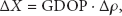
where
3.2. The Computational Formula of GDOP in WSN
3.2.1. The Cramer-Rao Lower Bound
The Cramer-Rao lower bound (CRLB) is widely used in parameter estimation. It can provide a lower limitation for the variance of any unbiased estimator. The expression of CRLB can be derived from the inverse matrix of the Fisher information metric (FIM) [26, 27]. It is assumed that the vector needs to be estimated as

The parameter

where

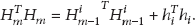
Let matrix
3.2.2. The Expression of GDOP
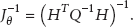
In the WSN, assuming that the location of the ith anchor node is

where

The covariance matrix Q can be represented as
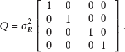
Here,

In the LOS environment, the measurement error obeys zero mean Gaussian distribution, so the covariance matrix can be expressed as
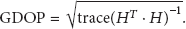
Involving matrix inversion and matrix multiplication, the computational complexity will be greatly increased when the dimensions of matrix H grow up [28].
Nodes are deployed in the 100 × 100 area, and the GDOP distribution maps are shown in Figures 2 and 3. It is clear that the GDOP inside the regular N-side polygon is quite smaller than that outside the regular N-side polygon. Furthermore, the smallest GDOP value
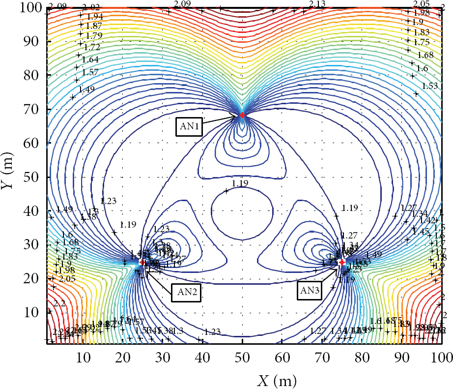
Equipotential line of GDOP distribution when there are three anchor nodes.

Equipotential line of GDOP distribution for four nodes.
3.3. GDOP Assisted Nodes Selection Algorithm
The traditional GDOP-based nodes selection algorithms usually calculate all the GDOP values of different combinations. The combination which has the smallest GDOP value will be selected to participate in the positioning. However, the computational complexity of this conception is too high that it is not suitable for practical application. In order to reduce the computational complexity, researchers have raised some methods such as neural networks, support vector machine, and genetic algorithm [30]. These methods can effectively reduce the computational complexity in different extent.
Theoretically, the more the nodes participate in the calculation, the lower the GDOP value of the combination will be, which represents a higher positioning accuracy. Our proposed GANS algorithm calculates the GDOP variation of different times. Through this method, we can obtain an anchor nodes subset which has the optimal GDOP value. Quite a few matrix inversions and matrix multiplication are avoided with GANS algorithm. Therefore, the GANS algorithm has a great advantage on direct nodes selection methods in terms of computational complexity.
Assume that
Assume that
where

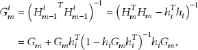
The equation above can also be expressed as
Let
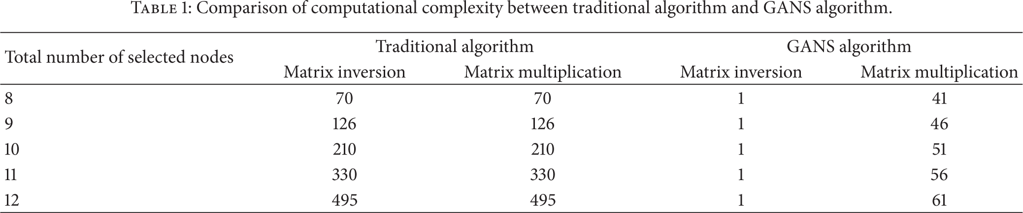
As we know, matrix multiplication and inversion require a lot of computation time. In the traditional GDOP-based nodes selection algorithm, n nodes will be selected from m anchor nodes. In order to select a subset which has the smallest GDOP, matrix multiplication and inversion should be executed for
Comparison of computational complexity between traditional algorithm and GANS algorithm.
3.4. Algorithm Design Process
The algorithm's design process is shown in Algorithm 1. When the mobile device locates in the scenario, the observation matrix of all nodes will be obtained firstly and the GDOP value of current position will be computed. The GDOP obtained will be compared with the threshold
Step 1. Calculate the current GDOP value; Step 2. Compare the GDOP with threshold If GDOP is larger than φ, go to Step 3; Else go to Step 5; Step 3. Calculate and sort the Step 4. Compare the If larger than δ, it should be kept to participate in positioning operations; If smaller than δ, it will be screened out; Step 5. Positioning with the LS method.
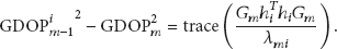
In order to reduce the communication traffic and the energy consumption, some certain nodes need to be removed from the positioning nodes set. As expounded in Section 3.3, the nodes which have weak influence on the positioning accuracy will be the key point focused on by the proposed algorithm. If the contribution
In this way, the number of the nodes participating in the localization calculation will be reduced. The computational complexity, communication, and energy consumption will all be reduced as a positive result.
4. Simulation Analysis and Verification
The WSN tracking area is set to be 100 m × 100 m, and the nodes are randomly distributed within a certain scope. As shown in Figure 4, three kinds of node distribution region are considered: (1) 50 * 80 region; (2) 100 * 100 region; (3) 50 * 50 region.

Three different nodes distributions and motion trail.
GDOP curves under three different node distributions are shown in Figure 5. When the nodes’ distribution obeys the first distribution, trajectory is not surrounded by the nodes and the node distribution is relatively dispersed. According to the previous discussion, the GDOP value will become larger when the trajectory is not surrounded by the nodes. In the region

GDOP curves under different node distributions.
Therefore, when the GDOP value varies in comparatively ideal interval, it is necessary to make sure that the anchor nodes throughout the region cover the whole area as large as possible. The area should be covered as much as possible where the mobile device possibly occurs.
Since the WSN is often used in dangerous environment such as industrial environment or in the military field, sensor nodes in such an environment cannot guarantee that the target area can be completely covered. Therefore, the first case mentioned above is closer to the actual situation. In the GANS algorithm validation, the first kind of nodes distribution is selected. Ten anchor nodes are deployed in a
The target's tracking trajectories with and without GANS algorithm are shown in Figure 6. Mobile device begins to move at (0, 0); then

Target tracking trajectory.
Figure 7 shows the number of nodes participating in the localization for both cases at different time. It can be seen that, most of the time, the number of nodes participating in the localization is less than 10. It is visible that the GANS node selection algorithm has a remarkably practical effect. As described in literature [4], the “unactivated” nodes will stay in “sleep” state and the “active” state will consume 100 times of energy than “sleep” state. Combined with the simulation results in Figure 4, the GANS node selection algorithm will save about 44.56% of the energy in this scenario.

Number of nodes in different time to participate in orientation.
Figure 8 shows the error curves in both cases. The positioning accuracy will have some inevitable loss because of the reduction of the number of nodes involved in the location calculation. This is just a result of the utilization of GANS algorithm. According to the simulation result, the positioning error without GANS algorithm is 2.145 m. Correspondingly, the positioning error with the GANS algorithm is 2.237 m. The loss in accuracy is not so obvious.

Positioning error curve.
The comparison of computational complexity between traditional nodes selection algorithm and the GANS nodes selection algorithm is shown in Figure 9.

Comparison of computational complexity.
As mentioned above, matrix multiplication and inversion will take up most of the operation time. Therefore, the execution time of these two kinds of complex operation is used to characterize the computational complexity of the algorithm. Since the principles of these two kinds of algorithm are not the same, the number of nodes selected by the GANS algorithm in each time will be used as the selected target numbers of the direct selection algorithm. It can be seen from the simulation result that the GANS algorithm has an obvious advantage in decreasing the computational complexity except for a few moments.
Figure 10 shows the case when the mobile device exactly passes through the node set including three sensor nodes. These nodes’ coordinates are (30, 25), (37, 25), and (55, 30), respectively, corresponding to the curve absence. When the mobile device passes through the node exactly, it is unable to get the observation vector H. Therefore, the GDOP value cannot be acquired through computation at this point. Under certain conditions, GDOP values may also change abruptly on the numerical value. This condition should be avoided for practical application.

GDOP curve with the mobile device passing through the node set exactly.
5. Conclusion
Aiming at node selection problem in wireless sensor networks with geometric constraint thought, we propose a GDOP assisted nodes selection algorithm. The GANS algorithm maintains the positioning accuracy when the system's energy consumption is effectively reduced. Simulation experiment is carried out in order to verify the effectiveness of our proposed algorithm. Results show that the algorithm has good positioning performance and lower computational complexity, which is superior to the traditional node selection algorithm based on GDOP. The GANS algorithm can be used in wireless sensor network for positioning and tracking moving targets. Since the mobile device's speed is relatively low, the false alarm and underreporting situation are not taken into consideration in the paper. In the following research, the influence of node's specific location on
Footnotes
Conflict of Interests
The authors declare that there is no conflict of interests regarding the publication of this paper.
Acknowledgments
This paper is supported by the National Natural Science Foundation of China (no. 61273078), the China Postdoctoral Science Foundation (no. 2012M511164), the Chinese Universities Scientific Foundation (N130404023), and the Liaoning Doctoral Startup Foundation (no. 20121004).