An Energy-Efficient Collaborative Target Tracking Framework in Distributed Wireless Sensor Networks

Abstract

Energy consumption and tracking accuracy are two significant issues for collaborative tracking in distributed wireless sensor networks (DWSNs). To obtain a benefit from those issues, most of the recent work tends to reduce the spatial redundancy, while ignoring utilizing the attribute of time redundancy. In this paper, a novel energy-efficient framework of collaborative signal and information fusion is proposed for acoustic target tracking. The proposed fusion algorithm is based on neural network aggregation model and Gaussian particle filtering (GPF) estimation. And the neural network based aggregation (NNBA) can reduce spatial and time redundancy. Furthermore, a fresh cluster head (CH) selection method demanding less task handover is also presented to decrease energy consumption. The analyzed framework coupled with simulations demonstrates its excellent performance in tracking accuracy and energy consumption.

1. Introduction

With the fast development of microelectromechanical system (MEMS), digital signal processing, and embedded computing, sensor nodes are becoming smaller and cheaper. Therefore, it is possible to deploy large-scale distributed wireless sensor networks (DWSNs) to “achieve quality through quantity” in many complex applications [1, 2].

However, challenges and difficulties also exist in target tracking DWSNs [3–5]: (1) sensor resources limitation [6] (especially communication bandwidth, energy, sensing range, and processing capabilities); (2) deployment and coordination of a mountain of sensors; (3) redundant data caused by similar measurements of adjacent sensors. Accomplishing the tracking task requires not only the methods for data fusion and collaborative signal and information processing (CSIP), but also an efficient scheme of energy consumption. In the literature, various researches have been proposed for target tracking in DWSNs [7].

In [8, 9], the nodes detect the mobile target and send measurements directly to the sink node so that it can estimate the target location using all data. But the centralized schemes, regarded as the first CSIP (CSIP1), depend on the sink node to collect and process measurements, as the sink node will consume a lot of energy and be apt to die quickly with constraint battery; the network lifetime is consequently shortened.

Energy aware probabilistic target localization algorithm for cluster-based WSN is proposed in [10]. Sensors detecting a target report a short message to the cluster head (CH). Then the CH localizes and determines the subset of sensors in the vicinity of target. This scheme can reduce communication bandwidth and save lots of energy. Nevertheless, the CH undertakes a heavy tracking task, which shortens its lifetime. The work in [11] proposed an adaptive dynamic cluster-based tracking (ADCT) protocol in which CHs are selected dynamically; meanwhile sensor nodes surrounding the target are waken up to construct a cluster with the target's moving in the network. Such scheme can be called the second CSIP (CSIP2). However, the election of the first CH is achieved by competition, which causes an additional burden in communication bandwidth.

A distributed predictive tracking (DPT) protocol for tracking moving objects with separate algorithms for nodes and CHs is presented in [12]. The CH adopts the target descriptor to identify target and predicts its next location. Then it informs predicted area CH who activates k sensors to sense the target. But most of the efforts have been spent on selecting the node nearest to the predicted target position for the CH. This scheme can be considered as the third CSIP (CSIP3).

Moreover, the work in [13] showed three algorithms for tracking a mobile target in WSNs utilizing cluster-based architecture, namely, adaptive head, static head, and selective static head. In [14], an intensive review was conducted to improve energy efficiency in collaborative target tracking in DWSNs.

Previous work was more focused on the spatial redundancy of the distributed sensor network for target tracking. However, the study on the time redundancy is still important. The purpose of this paper is to design a novel energy-efficient collaborative signal and information fusion processing (CSIFP) framework for acoustic target tracking in DWSNs, to collaboratively estimate the position and velocity of a moving target. In our framework, sensor nodes detecting a target are activated and dynamically form a cluster around the target. Each member node transfers the deredundant data to the CH. CH aggregates and processes these messages to estimate the current state of the target and reports the result to the sink. The CH is reselected relying on certain rule in Sections 4.1 and 4.2. To estimate the target position, the Gaussian particle filter (GPF) algorithm [15] is adopted. Compared with the particle filter (PF) [16–18], it omits resampling to reduce the computational complexity and avoid transmitting all particles and weights when task handover happens. Furthermore, the neural network based aggregation (NNBA) model relies on the cooperation of the nodes, which can reduce the spatial and time redundancy.

The paper is organized as follows. Section 2 presents the system assumptions and the system models. Section 3 proposes the framework of the distributed collaborative target tracking framework is illustrated. Section 4 discusses a neuron network based aggregation model for target tracking. Section 5 describes the simulation environment and Section 6 shows and analyzes the results. Finally, Section 7 summarizes the work and gives a conclusion.

2. Problem Statements

2.1. Assumptions

First, several assumptions about the sensor nodes and the underlying networks are defined:

• (i)

All sensor nodes are assumed to be homogeneous and synchronized. Cluster-based structure is used for the nodes' deployment. The CH is responsible for task decision, data fusion, and routing tracking results to the sink node.

(ii)

Each node knows its own position after initial deployment.

(iii)

The maximum communication range of each sensor node is twice larger than the maximum sensing range; that is $R_c\ge \mathrm{2}{R}_s$ . This guarantees that all activated nodes can communicate with CH.

(iv)

All sensor nodes are initialized with the same fixed amount of battery energy.

(v)

As the paper focuses on the energy consumption of target tracking in DWSNs, the energy consumed by sensor nodes in the sleeping state is not considered. However, it does not mean that the energy consumption of idle sensor nodes can always be ignored.

2.2. Target Dynamic Model and Measurement Model

Target tracking aims to estimate the real-time state of a moving object, which is mainly based on the target dynamic models. The appropriate models can not only describe the evolution of the target state with respect to time, but also represent a large number of observations, reducing the data transmission in the DWSNs [19].

The target state is denoted by a four-dimensional vector in 2D Cartesian coordinate plane:

$$\begin{array}{cc}& {\mathbf{x}}_k={\left[\begin{array}{cccc}{\xi }_k& \dot{{\xi }_k}& {\eta }_k& \dot{{\eta }_k}\end{array}\right]}^T,\end{array}$$

(1)

where ${\xi }_k$ and ${\eta }_k$ denote the target position in x-axis and y-axis at time $t_k$ and $\dot{{\xi }_k}$ and $\dot{{\eta }_k}$ denote the corresponding velocities.

We describe the target dynamic model with addictive noise as the state-space model in the following form:

$$\begin{array}{cc}& {\mathbf{x}}_k=f_k\left({\mathbf{x}}_{k-1},{\mathbf{u}}_{k-1}\right)+{\mathbf{w}}_k,\end{array}$$

(2)

$$\begin{array}{cc}& {\mathbf{z}}_k=h_k\left({\mathbf{x}}_k\right)+{\mathbf{v}}_k,\end{array}$$

(3)

where ${\mathbf{x}}_k$ , ${\mathbf{z}}_k$ , and ${\mathbf{u}}_k$ are the target state, observation, and control input vectors, respectively, at the discrete time $t_k$ , ${\mathbf{w}}_k$ is the system noise at $t_k$ , and ${\mathbf{v}}_k$ is the observation noise, assumed to be statistically independent from ${\mathbf{w}}_k$ . $f_k$ and $h_k$ are state transition and observation functions, which are vector valued (possibly time-varying).

For nearly constant velocity (CV) or white noise acceleration model [19], ${\mathbf{u}}_k$ is approximated to zero, and (2) can be rewritten by

$$\begin{array}{cc}& {\mathbf{x}}_k=F_k{\mathbf{x}}_{k-1}+{\mathbf{w}}_k,\end{array}$$

(4)

where

$$\begin{array}{cc}& F_k=\left[\begin{array}{cccc}\mathrm{1}& T& \mathrm{0}& \mathrm{0}\\ \mathrm{0}& \mathrm{1}& \mathrm{0}& \mathrm{0}\\ \mathrm{0}& \mathrm{0}& \mathrm{1}& T\\ \mathrm{0}& \mathrm{0}& \mathrm{0}& \mathrm{1}\end{array}\right].\end{array}$$

(5)

Note that T is the sampling period.

2.3. Measurement Model [20–22]

Energy based acoustic sensors are widely used in DWSNs due to low cost and universality. The intensity of the source attenuates at a rate that is inversely proportional to the distance from the source. Given $N_s$ sensors, the signal intensity measured on the nth sensor is given by

$$\begin{array}{l}{z}_{k,n}=h_k\left({\mathbf{x}}_k\right)+v_{k,n}=g_n·\frac{s}{{\parallel {\mathbf{r}}_t-{\mathbf{r}}_n\parallel }^{\alpha }}+v_{k,n},\\ \hspace{1em}\hspace{1em}\hspace{1em}\hspace{1em}\hspace{1em}\hspace{1em}\hspace{1em}\hspace{1em}\hspace{1em}n=\mathrm{1,2},\dots ,N_s,\end{array}$$

(6)

where s is the strength of the acoustic emitted by the target during T. The vectors ${\mathbf{r}}_t$ and ${\mathbf{r}}_n$ denote the coordinates of the target and the nth sensor at time step $t_k$ , respectively. $\parallel {\mathbf{r}}_t-{\mathbf{r}}_n\parallel$ is the Euclidean distance between the nth sensor node and the target. $g_n$ is sensor gain factor of the nth sensor, which can be measured during sensor calibration. α is the intensity decay factor. In [21], it is shown that the effective decay, α, is approximately 2 and this value is assumed for this paper. $v_{k,n}$ is white Gaussian measurement noise, $v_{k,n}~N(0,{\sigma }_{vn}^2)$ , independent of $w_k$ , and independent of other sensors' noise. In practice, ${\sigma }_{vn}^2$ can be estimated based on the measurements when the acoustic source is absent. For concise notation, ${\sigma }_{vn}^2$ is assumed to be identical for all sensor nodes, ${\sigma }_{vn}^2={\sigma }_v^2$ for $\mathrm{1}\le n\le N_s$ , and it is assumed to be known.

3. Distributed Collaborative Target Tracking Framework

In this paper, we develop an energy-efficient distributed collaborative target tracking framework.

This effective framework involves four modules: the tracking task initialization, CH election, node selection, and tracking task handover. Before specifying the aforementioned contents, several messages are listed in Table 1.

Table 1

Messages used in the target tracking framework.

Message type	Purpose
CHInfoMesg	CH informs its member nodes to join this cluster
CHHandoverMesg	CH transmits the parameters to the new CH when task handover happens
DataMesg	Node sends their measurements to CH
DataDegradeMesg	Nodes send their information without measurements to CH
TargetToSinkMesg	CH transmits the target position estimation to the sink
TargetDegradeMesg	CH transmits the result to the sink

3.1. Tracking Task Initialization

Assume that a network with 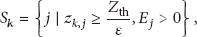$N_s$ sensors is deployed on a 2D area. For a given acoustic energy sensor node, it can detect a target once the acoustic intensity measurement exceeds a threshold, $Z\text{th}$ , corresponding to the calculated strength at the maximum sensing distance $R_s$ . Sensor nodes detecting the target are activated, whereas the other nodes remain in the sleeping state for saving energy. Considering the influence of the measurement noise, we define a set of candidate nodes whose measurements of acoustic intensity are not lower than $Z_{\text{th}}/\epsilon$ and remaining energy is greater than zero. Only the candidate nodes could participate in the target tracking process and transmit the measurements to the CH. The candidate nodes set S is denoted as follows:

$$\begin{array}{cc}& S_k=\left\{j\hspace{0.17em}|\hspace{0.17em}{z}_{k,j}\ge \frac{Z_{\text{th}}}{\epsilon },E_j>\mathrm{0}\right\},\end{array}$$

(7)

where $z_{k,j}$ is the measurement of sensor node j at time $t_k$ and the energy threshold $Z_{\text{th}}$ is $g·(s/R_s^2)$ . Parameter $\epsilon \in (\mathrm{0},\mathrm{1}]$ is customized, and a bigger ε means more candidate nodes will be chosen. $E_j$ is the remaining energy of the node j, and $R_c$ is the communication radius.

At initial time step as well as the target detection restart phase, each candidate sensor node starts a timer $T_C$ and will broadcast CHInfoMesg after the timer expires. The length of $T_C$   is

$$\begin{array}{cc}& T_C\propto \text{dis}\left(j,x\right)=g·\frac{s}{z_{k,j}}.\end{array}$$

(8)

According to (6), the sensor with the largest measurement is nearest to the target; thus, $T_C$ is the smallest. So the sensor node nearest to the target will first send its CHInfoMesg. The other nodes which have received this message register the broadcaster as their CH, terminate the timer, and give up broadcasting message. Through the above process, the candidate closest to the target is elected to be the CH. The cluster member nodes transmit their observation to CH, and the CH aggregates the collected information and performs the tracking task using GPF.

3.2. CH Selection

It is expectable that CHs will consume much more energy than others because they undertake more burdensome tasks. For balancing the energy consumption, each node needs to take turn as CH by certain scheduling algorithm. However, CH rotation process consumes a lot of energy for transmitting message between CHs. Therefore, we propose a novel CH selection scheme considering these two factors.

At time $t_{k-1}$ , it is assumed that the CH is ${\text{CH}}_{k-1}$ . According to the predicted target position at time $t_k$ and cluster members information, ${\text{CH}}_{k-1}$ builds a candidate CH set $C_k$ :

$$\begin{array}{cc}& C_k=\left\{j\hspace{0.17em}|\hspace{0.17em}\text{dis}\left(j,{\tilde{\mathbf{x}}}_k\right)\le \rho ·R_s,\hspace{0.17em}{E}_j\ge E_{\text{th}}\right\},\end{array}$$

(9)

where   $\rho \in [\mathrm{0,1}]$ is customized and a smaller ρ means CH changes more frequently. $E_j$ is the remaining energy of node j, and $E_{\text{th}}$ is the threshold energy. If $E_j$ is lower than $E_{\text{th}}$ , a node is not suitable for being a cluster head.

The current CH checks itself whether it belongs to the candidate set $C_k$   or not. If so, it will continue taking charge of the tracking task; otherwise, it will hand over the CHHandoverMesg including tracking information and necessary parameters to ${\text{CH}}_k$ . In order to select an appropriate new CH, we define the attraction force $F_j$ of the node j, exerting on the current CH. The larger value means the node j has greater probability to be chosen as next CH:

$$\begin{array}{cc}& F_j=\alpha ·F_{\text{dir},j}+\beta ·F_{\text{dis},j}+\gamma ·F_{\text{power},j}.\end{array}$$

(10)

Note that $F_{\text{dir},j}$ , $F_{\text{dis},j}$ , and $F_{\text{power},j}$ are the direction attraction component force, distance attraction component force, and power attraction component force exerting on ${\text{CH}}_{k-1}$ by node j, respectively. α, β, and γ are three nonnegative constants which adjust the ratios of the above three component forces, and $\alpha +\beta +\gamma =\mathrm{1}$ . Consider the following.

• (i)

Direction attraction component force $F_{\text{dirt},j}$ : the direction from the current cluster head ${\text{CH}}_{k-1}$ to node j and the direction from ${\text{CH}}_{k-1}$ to the predicted target position ${\tilde{\mathbf{x}}}_k$ are more closer, which means that the node j is nearly on the direction of the target motion and has a high probability to be the cluster head at time step $t_k$ . We define the cosine value of this angle to indicate the force $F_{\text{dirt},j}$ :

$$\begin{array}{cc}& F_{\text{dir},j}=\{\begin{array}{cc}\frac{〈{\mathbf{r}}_{{\text{CH}}_{k-1}}\mathbf{,}\hspace{0.17em}{\mathbf{r}}_j〉}{\parallel {\mathbf{r}}_{{\text{CH}}_{k-1}}\parallel ·\parallel {\mathbf{r}}_j\parallel },\hfill & \text{if}\mathrm{\hspace{0.17em}\hspace{0.17em}}j\in S_{k-\mathrm{1}},\hfill \\ \mathrm{0},\hfill & \text{else},\hfill \end{array}\end{array}$$

(11)

where ${\mathbf{r}}_{{\text{CH}}_{k-1}}$ is a vector from ${\text{CH}}_{k-1}$ to the predicted target position ${\tilde{\mathbf{x}}}_k$ and ${\mathbf{r}}_j$ is vector from the current cluster head ${\text{CH}}_{k-1}$ to node j. $〈{\mathbf{r}}_{{\text{CH}}_{k-1}},{\mathbf{r}}_j〉$ is the inner product. $\parallel {\mathbf{r}}_{{\text{CH}}_{k-1}}\parallel$ and $\parallel {\mathbf{r}}_j\parallel$ represent the length of ${\mathbf{r}}_{{\text{CH}}_{k-1}}$ and ${\mathbf{r}}_j$ , respectively.

(ii)

Distance attraction component force $F_{\text{dis},j}$ : for the sake of reducing the frequency of CH reselection, we choose the candidate node as far as the current CH on the premise of an acceptable tracking accuracy. $F_{\text{dis},j}$ is defined as follows:

$$\begin{array}{cc}& F_{\text{dis},j}=\{\begin{array}{cc}\frac{{\text{dis}\left(j,{\text{CH}}_{k-\mathrm{1}}\right)}^{\mathrm{2}}}{R_c^{\mathrm{2}}},\hfill & \text{if}\mathrm{\hspace{0.17em}\hspace{0.17em}}\text{dis}\left(j,{\text{CH}}_{k-\mathrm{1}}\right)<R_c,\hfill \\ \mathrm{0},\hfill & \text{else},\hfill \end{array}\mathrm{\hspace{0.17em}\hspace{0.17em}}\end{array}$$

(12)

where $\text{dis}\hspace{0.17em}(j,{\text{CH}}_{k-1})$ is the Euclidian distance between the node j and the current cluster head ${\text{CH}}_{k-1}$ and $R_c$ is the communication radius.

(iii)

Power attraction component force $F_{\text{power},j}$ : $F_{\text{power},j}$ is defined to indicate the node battery level, which is given by

$$\begin{array}{cc}& F_{\text{power},j}=\{\begin{array}{cc}\frac{E_j}{E_{\mathrm{0}}},\hfill & \text{if}\mathrm{\hspace{0.17em}\hspace{0.17em}}{E}_j\ge E_{\text{th}}\hfill \\ \mathrm{0},\hfill & \text{else},\hfill \end{array}\end{array}$$

(13)

where $E_0$ is the initial energy of the node j.

Finally, ${\text{CH}}_k$ is selected according to the following rule:

$$\begin{array}{l}{\text{CH}}_k\\ \hspace{0.5em}=\{\begin{array}{ll}{\text{CH}}_{k-\mathrm{1}},\hfill & {\text{CH}}_{k-\mathrm{1}}\in C_k,\hfill \\ \left\{j\hspace{0.17em}|\hspace{0.17em}\text{dis}\left(j,{\text{CH}}_{k-\mathrm{1}}\right)<R_c,\arg \hspace{0.17em}\max \left(F_j\right)\right\},\hfill & \text{otherwise}.\hfill \end{array}\end{array}$$

(14)

Noting that it is possible for multiple candidate nodes to have the same maximum attraction force, in this case, we will select one node randomly among these nodes as the new CH.

3.3. Member Node Selection

The node selection determines the total energy consumption and data fusion accuracy, which has a significant impact on the performance of the whole sensor network.

To implement an optimal cluster with member nodes, more nodes should be selected to improve the tracking accuracy. On the other hand, fewer nodes should be selected to reduce the energy consumption for transmission. So we need to make a compromise. Considering the influence of measurement noise, we choose the nodes located in the communication range of the current CH from the set of candidate nodes $S_k$ . The set of member nodes are denoted by

$$\begin{array}{cc}& N_k=\left\{j\hspace{0.17em}|\hspace{0.17em}\text{dis}\left(j,\text{CH}\right)\le R_c,j\in S_k\right\},\end{array}$$

(15)

where $\text{dis}\hspace{0.17em}(j,\text{CH})$ is the distance between the node j and the position of the current CH at $t_k$ . The constraint $\text{dis}\hspace{0.17em}(j,\text{CH})\le R_c$ is resistant to the measurement noise.

3.4. Tracking Task Handover

Once the target is far away from the current CH and ${\text{CH}}_{k-1}\notin C_k$ , ${\text{CH}}_{k-1}$ cannot efficiently manage. ${\text{CH}}_{k-1}$ should hand over the tracking task to a new CH. This operation can not only shut down the old nonsignificant cluster nodes to save energy in time but also improve the tracking accuracy.

The current CH selects a member node from $C_k$ as the new CH, ${\text{CH}}_k$ , which is along the direction of estimated target motion as well as far away from the current CH. Then ${\text{CH}}_{k-1}$ sends a CHHandoverMesg message to ${\text{CH}}_k$ . This message contains the current target state estimation as well as some necessary parameters. After receiving the CHHandoverMesg from ${\text{CH}}_{k-1}$ , ${\text{CH}}_k$ will continue to take charge of the target tracking task and broadcast CHInfoMesg to inform its cluster members.

3.5. Working Scheduling

The distributed collaborative target tracking framework of the CH and member nodes is shown in Figure 1. Consider the following.

• (i)

The cluster head: CH is generated or reselected according to (14), and it broadcasts CHInfoMesg message to inform its cluster members. CH receives the DataMesg packet or DataDegradeMesg packet from its members, then chooses three messages with the biggest acoustic intensity measurement, and performs the GPF algorithm described in Section 4.2 to estimate the current target state and predict the possible state at next time step. The CH also takes charge of sending the tracking results to the sink node. If the difference between estimated target position at $t_k$ and the one at $t_{k-1}$ is greater than the threshold $\theta \mathrm{2}$ , CH uploads TargetToSinkMesg packet containing packet type, CH ID, tracking result; otherwise, CH sends TargetDegradeMesg packet without tracking result. The sink keeps the previous value once receiving TargetDegradeMesg.

(ii)

Member node j: after receiving CHInfoMesg from the current CH, it checks whether it belongs to the member nodes set $N_k$ . If so, the node transfers DataMesg including packet type, ID, and measurement to the CH. Otherwise it goes to sleep state. When the difference of the calculated distance between the node j and the target at $t_k$ and $t_{k-1}$ is smaller than difference threshold $\theta \mathrm{1}$ , it sends a DataDegradeMesg, omitting measurement. The CH holds its previous measurement once receiving DataDegradeMesg.

Figure 1

Flowchart of the distributed collaborative tracking scheme.

Note that, at any time, only several sensor nodes in the vicinity of the target need to collect the acoustic signal and the others keep sleeping.

The CH and member nodes run in the neural network based aggregation tracking model, which will be expatiated in Section 4.

4. Neural Network Based Aggregation Tracking Model

This section details the fusion processing algorithm based on neural network based aggregation tracking model. It combines the neural network of multilayer perceptron with clustering routing structure. This algorithm reduces time redundancy and spatial redundancy to reduce the traffic, save energy, and prolong the network lifetime.

4.1. Collaborative Target Tracking Scheme

Figure 2 gives the diagram of NNBA model structure [23], which uses four-perceptron neural network. For DWSNs, each sensor node works as an underlying neuron; CH is like a central neuron, and the whole network is a complex neuron network system.

Figure 2

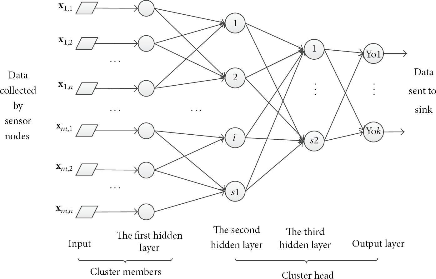
NNBA model architecture.

Cluster member nodes are in the input layer and the first hidden layer. CH nodes are in the second and the third hidden layer and output layer. For instance, each cluster with n members collects data of m species by different types. Consequently, this NNBA model has $n\times m$ input layer nodes and the same number of first hidden layer neurons. Here, we only use the acoustic sensor, so $m=1$ . The quantity of neurons in the second hidden layer, the third hidden layer, and the output layer can be adjusted by the users according to the practical application. The hidden layers have no inevitable relationship with n. It only deals with separate data of different types and need not be fully connected between the first and the second hidden layer. So do the second and the third hidden layer. But the treated data between the third hidden layer and output layer can be integrated, for they are full-connected.

According to this NNBA model, firstly sensor nodes collect the acoustic intensity measurements from the target and preprocess them according to the neuron function of the first hidden layer. Then the nodes send the results to the CH. The CH further processes to track the target using GPF algorithm detailed in Section 4.2. GPF is embedded in the second hidden layer, the third hidden layer, and output layer neurons. Finally, the CH transfers the estimated target state to the sink. Note that neural network model can do some modification according to the specific requirements in various applications.

4.2. Gaussian Particle Filter

Recalling the theory of particle filtering [16–18], we estimate the target a posteriori distribution $p({\mathbf{x}}_{0:k}\hspace{0.17em}|\hspace{0.17em}{\mathbf{z}}_{1:k})$ of ${\mathbf{x}}_{0:k}$ , by approximating it with a random measure composed of particles ${\mathbf{x}}_k^i$ and weights $w_k^i$ , where i is a particle index. We denote it by $\mathrm{\Xi }={\{{\mathbf{x}}_{0:k}^i,w_k^i\}}_{i=1}^N$ with N being the number of particles. At each time step $t_k$ , the particle filter carries out the following operations: (1) selection of most promising particle set, (2) particle propagation, (3) computation of particle weights, and (4) state estimation.

The Gaussian particle filter (GPF) [15] approximates the posterior $p({\mathbf{x}}_k\hspace{0.17em}|\hspace{0.17em}{\mathbf{z}}_{0:k})$ by a Gaussian pdf, whose mean and covariance are calculated from the weighted particle set. In contrast to the standard PF [16–18], GPF algorithm does not require the process of resampling, which reduces the computational complexity.

Assume that the initial target state is known and its distribution accords with Gaussian distribution $N({\mathbf{x}}_{\mathrm{0}};{\stackrel{-}{\mathbf{x}}}_{\mathrm{0}},{\stackrel{-}{P}}_{\mathrm{0}})$ . The steps of GPF algorithm are described as follows.

• (1)

Time step $t=0$ ;

 

Initialize the parameter: ${\mathit{\mu }}_0={\stackrel{-}{\mathbf{x}}}_0,{\Sigma }_0={\stackrel{-}{P}}_0$ .

(2)

Time Update (Prediction)

 

Time step $t_{k-1}$ ;

• (a)

Draw samples from the distribution $p({\mathbf{x}}_{k-1})~N({\mathbf{x}}_{k-1};{\mathit{\mu }}_{k-1},{\Sigma }_{k-1})$ , and denote them as ${\{{\mathbf{x}}_{k-1}^i\}}_{i=1}^N$ .

(b)

For $i=1,\dots ,N$ , sample from $p({\mathbf{x}}_k\hspace{0.17em}|\hspace{0.17em}{\mathbf{x}}_{k-1}={\mathbf{x}}_{k-1}^i)$ to obtain predicted particles' set ${\{{\mathbf{x}}_{k\hspace{0.17em}|\hspace{0.17em}k-1}^i\}}_{i=1}^N$ .

(c)

Calculate the mean ${\stackrel{-}{\mathbf{x}}}_{k\hspace{0.17em}|\hspace{0.17em}k-1}$ and covariance ${\stackrel{-}{P}}_{k\hspace{0.17em}|\hspace{0.17em}k-1}$ as

$$\begin{array}{cc}& {\stackrel{-}{\mathbf{x}}}_{k\hspace{0.17em}|\hspace{0.17em}k-\mathrm{1}}=\frac{\mathrm{1}}{N}{\displaystyle \sum }_{i=\mathrm{1}}^N{\mathbf{x}}_{k\hspace{0.17em}|\hspace{0.17em}k-\mathrm{1}}^i,\\ {\stackrel{-}{P}}_{k\hspace{0.17em}|\hspace{0.17em}k-\mathrm{1}}=\frac{\mathrm{1}}{N}{\displaystyle \sum }_{i=\mathrm{1}}^N\left({\stackrel{-}{\mathbf{x}}}_{k\hspace{0.17em}|\hspace{0.17em}k-\mathrm{1}}-{\mathbf{x}}_{k\hspace{0.17em}|\hspace{0.17em}k-\mathrm{1}}^i\right){\left({\stackrel{-}{\mathbf{x}}}_{k\hspace{0.17em}|\hspace{0.17em}k-\mathrm{1}}-{\mathbf{x}}_{k\hspace{0.17em}|\hspace{0.17em}k-\mathrm{1}}^i\right)}^T.\end{array}$$

(16)

(3)

Measurement Update

 

Time step $t_k$ ;

• (a)

Draw samples from the importance function $q({\mathbf{x}}_k\hspace{0.17em}|\hspace{0.17em}{\mathbf{z}}_{0:k})$   , and denote them as ${\{{\mathbf{x}}_k^i\}}_{i=1}^N$ .

(b)

Obtain the respective particle weights by

$$\begin{array}{cc}& w_k^i=\frac{p\left({\mathbf{z}}_k\hspace{0.17em}|\hspace{0.17em}{\mathbf{x}}_k^i\right)N({\mathbf{x}}_k^i;{\stackrel{-}{\mathbf{x}}}_{k\hspace{0.17em}|\hspace{0.17em}k-\mathrm{1}},{\stackrel{-}{P}}_{k\hspace{0.17em}|\hspace{0.17em}k-\mathrm{1}})}{q\left({\mathbf{x}}_k\hspace{0.17em}|\hspace{0.17em}{\mathbf{z}}_k\right)}.\end{array}$$

(17)

(c)

Normalize the weights as

$$\begin{array}{cc}& w_k^i=\frac{w_k^i}{{\sum }_{i=\mathrm{1}}^N{w}_k^i}.\end{array}$$

(18)

(d)

Calculate the mean ${\mathit{\mu }}_k$ and the covariance ${\Sigma }_k$ of approximate Gaussian distribution by

$$\begin{array}{cc}& {\mathit{\mu }}_k=\frac{\mathrm{1}}{N}{\displaystyle \sum }_{i=\mathrm{1}}^N{\mathbf{x}}_k^i,\\ {\Sigma }_k=\frac{\mathrm{1}}{N}{\displaystyle \sum }_{i=\mathrm{1}}^N\left({\mathit{\mu }}_k-{\mathbf{x}}_k^i\right){\left({\mathit{\mu }}_k-{\mathbf{x}}_k^i\right)}^T.\end{array}$$

(19)

(e)

Estimate the target position at time $t_k$ and predict the target position at time $t_{k+1}$ by

$$\begin{array}{cc}& {\widehat{\mathbf{x}}}_k={\mathit{\mu }}_k,\hspace{1em}\hspace{1em}{\tilde{\mathbf{x}}}_{k+\mathrm{1}}=F_{k+\mathrm{1}}·{\widehat{\mathbf{x}}}_k.\end{array}$$

(20)

4.3. NNBA Neuron Model

4.3.1. The First Hidden Layer

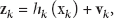
Figure 3 shows the first hidden layer neuron model. The ith input is the measurement ${\mathit{z}}_{k,i}$ of node i. The input function, which is a weighted sum, actually becomes an identity function. Because each of the neuron only has one input signal, the operation result is input signal itself. The process area has two functions. The first calculates the difference between the measurement and previous record if the measurements satisfy $p_1\ge Z_{\text{th}}/\epsilon$   ( $\epsilon \in (\mathrm{0,1}]$ ). Based on the measurement model (6), the sensor data is valuable when the distance $\parallel {\mathbf{r}}_t-{\mathbf{r}}_n\parallel$ between sensor node and the target is within certain limits, so the threshold $Z_{\text{th}}/\epsilon$ guarantees the accuracy of measurement. And the second function checks and decides whether to record this current input data. The output function is a specific threshold function, which is different from the standard threshold function with output 0 or 1. This function outputs $a2(k)$ if $a1(k)\ge \theta \mathrm{1}$ , else output none, to reduce the time redundancy.

Figure 3

NNBA model first hidden layer neuron function.

4.3.2. The Second Hidden Layer

The second hidden layer on the CH merges with the GPF algorithm (see Figure 4). CH chooses three maximum measurements and puts them in neurons, respectively, in the second hidden layer. According to GPF algorithm, CH draws samples ${\{{\mathbf{x}}_{k-1}^i\}}_{i=1}^N$ from the distribution $p({\mathbf{x}}_{k-1})~N({\mathbf{x}}_{k-1};{\mathit{\mu }}_{k-1},{\Sigma }_{k-1})$ , in which the mean ${\mathit{\mu }}_{k-1}$ and covariance ${\Sigma }_{k-1}$ can be computed by (16). In the process function, each neuron continues to complete the time update process, draws samples from the importance function $q({\mathbf{x}}_k\hspace{0.17em}|\hspace{0.17em}{\mathbf{z}}_{0:k})$ , and obtains the respective particle weights by (17) based on input parameter p, ${\mathit{\mu }}_{k-1},{\Sigma }_{k-1}$ and the same particle set ${\{{\mathbf{x}}_{k-1}^i\}}_{i=1}^N$ . At last, each neuron outputs its own normalization weights.

Figure 4

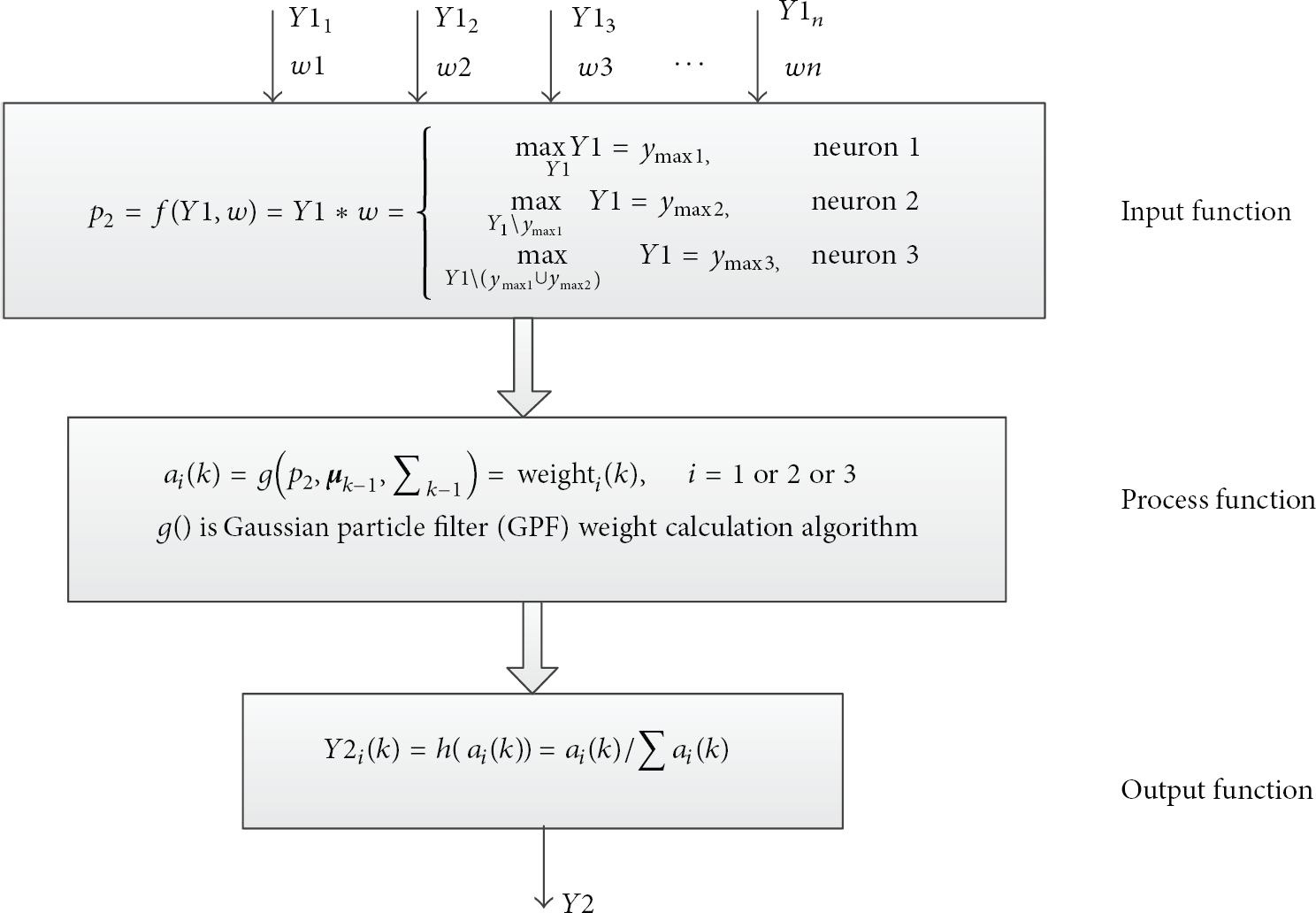
NNBA model second hidden layer neuron function.

4.3.3. The Third Hidden Layer

One neuron is used to complete the subsequent GPF algorithm in the third hidden layer. As shown in Figure 5, CH averages value of the input $Y2$ , the weight of the three particle sets. The process function is used to estimate the target position ${\widehat{\mathbf{x}}}_k$ and covariance ${\Sigma }_k$ according to (19). The output of the function equals the estimated target position ${\widehat{\mathbf{x}}}_k$ represented by $Y3$ , which will be transferred to the output layer.

Figure 5

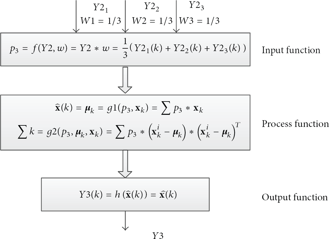
NNBA model third hidden layer neuron function.

The GPF tracking algorithm is completely performed by the second and third hidden layer. Note that these two can be combined into a union, in which case the input data should be aggregated into a vector.

4.3.4. The Output Layer

The output neuron model resembles the input neuron. Different from the input neuron, the output neuron model can be multi-input neuron, which is determined by the sensor type. In this study, only acoustic energy sensor is used, so there is one neuron in output layer.

As Figure 6 shows, CH compares the input $p_o$ and $a(k-1)$ . If the difference exceeds the threshold $\theta \mathrm{2}$ , that is, $\Delta (k)\ge \theta \mathrm{2}$ , CH outputs $p_o$ and sends the TargetToSinkMesg containing target state estimation to the sink; otherwise, the neuron outputs none, and CH sends TargetDegradeMesg message to the sink. The shortened messages reduce traffic and lower the energy consumption especially when the target stops or moves slowly.

Figure 6

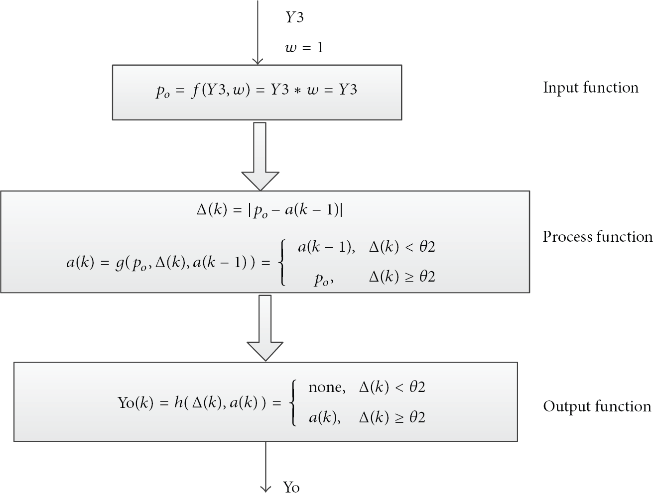
NNBA model output layer neuron function.

Neurons in NNBA algorithm need some operation parameters (such as weight, thresholds, etc.) at runtime; as a result, the neuron network model parameters should be trained after the clustering and CH election. In general, the neuron network can learn, train, and adjust these parameters by itself. However, due to the limited resources, it is unadvisable to do the training inside the DWSNs. Hence, NNBA model does this training process at the sink out of the neuron network. And then the sink would send the model parameters to the CHs and member nodes.

5. Simulation Environment and Setup

In this section, we build a simulation platform to evaluate the performance of the proposed distributed collaborative target tracking framework. Firstly, we describe our simulation environment and parameters. Then we define the performance metrics to compare the proposed algorithm and others' work.

5.1. Simulation Environment

We simulate a wireless sensor network with $N_s=\mathrm{200}$ randomly deployed acoustic sensors to monitor a 800 m × 800 m square field. All the sensor nodes within the monitoring region (excluding sink) have same structure and can detect the target within the sensing range. The measurements collected by sensor nodes are corrupted by zero-mean i.i.d. Gaussian noise with variance ${\sigma }_v^2=0.00005$ . The parameters of the measurement model in (6) are $s=\mathrm{1000}$ , $g_n=\mathrm{1}$ . Besides that, for the CH selection phase in the proposed framework, weight constants in (10) are $\alpha =\mathrm{0.4}$ , $\beta =\mathrm{0.3}$ , and $\gamma =\mathrm{0.3}$ ; energy threshold is set to 10% of the initial battery level; namely, $E_{\text{th}}=0.1\times E_0$ .

We should also determine the thresholds ε and ρ, for they are playing an important role in selecting the candidate nodes and CH. The bigger the ε is, the higher the tracking accuracy is, but the more energy the whole network consumes. The bigger the ρ is, the less frequently the CH hands over, and the more energy consumption the whole network has. On the other hand, the tracking accuracy is not closely tied with ρ. According to large number of experiment results, a best tradeoff between good tracking accuracy and low energy consumption is achieved in the case of $\epsilon =0.64$ , $\rho =0.7$ .

Simulation parameters are summarized in Table 2.

Table 2

The set of the simulation parameters.

Parameter	Value
Monitoring region	800 m × 800 m
Number of nodes $\text{Ns}$	200
Sink location	(400, 400) in the middle of the area
Sensing radius $\text{Rs}$	150 m
Communication radius $\text{Rc}$	300 m
Capability of power $E_0$	1 J
$E_{\text{elec}}$	50 nJ/bit
${\mathrm{\hspace{0.17em}\hspace{0.17em}}\mathrm{\hspace{0.17em}\hspace{0.17em}}\mathrm{\epsilon }}_{\text{fs}}$	10 pJ/bit/m2
${\mathrm{\hspace{0.17em}\hspace{0.17em}}\mathrm{\hspace{0.17em}\hspace{0.17em}}\mathrm{\epsilon }}_{\text{mp}}$	0.0013 pJ/bit/m4
Member nodes threshold $\mathrm{\epsilon }$	0.64
CH threshold $\mathrm{\rho }$	0.7

5.2. Performance Metrics

5.2.1. Tracking Performance

Assume a target moves into the monitoring field at time $t=0$ with initial state ${[\mathrm{50}\mathrm{\hspace{0.17em}\hspace{0.17em}}\mathrm{6}\mathrm{\hspace{0.17em}\hspace{0.17em}}\mathrm{0}\mathrm{\hspace{0.17em}\hspace{0.17em}}\mathrm{6}]}^T$ . The simulation tracking time is $T_{\text{sim}}=\mathrm{100}$ . The system process noise $w_k$ is assumed as zero-mean Gaussian distribution with variance ${\sigma }_w^2=\mathrm{diag}([0.125\hspace{0.17em}\hspace{0.17em}0.5\hspace{0.17em}\hspace{0.17em}0.125\hspace{0.17em}\hspace{0.17em}0.5])$ . The number of particles used in each algorithm is $M=\mathrm{600}$ .

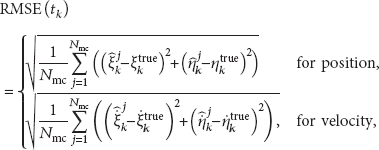
To evaluate the tracking performance for different algorithms, we calculate the root of mean square errors (RMSEs) of target position and velocity estimations at each time step under 50 Monte Carlo runs. The RMSEs metric [24] is defined as

$$\begin{array}{l}\text{RMSE}\left(t_k\right)\\ =\{\begin{array}{ll}\sqrt{\frac{\mathrm{1}}{N_{\text{mc}}}{\displaystyle \sum }_{j=\mathrm{1}}^{N_{\text{mc}}}\left({\left({\widehat{\xi }}_k^j-{\xi }_k^{\text{true}}\right)}^{\mathrm{2}}+{\left({\widehat{\eta }}_k^j-{\eta }_k^{\text{true}}\right)}^{\mathrm{2}}\right)}\hfill & \text{for}\mathrm{\hspace{0.17em}\hspace{0.17em}}\text{position},\hfill \\ \sqrt{\frac{\mathrm{1}}{N_{\text{mc}}}{\displaystyle \sum }_{j=\mathrm{1}}^{N_{\text{mc}}}\left({\left({\widehat{\dot{\xi }}}_k^j-{\dot{\xi }}_k^{\text{true}}\right)}^{\mathrm{2}}+{\left({\widehat{\dot{\eta }}}_k^j-{\dot{\eta }}_k^{\text{true}}\right)}^{\mathrm{2}}\right),}\hfill & \text{for}\mathrm{\hspace{0.17em}\hspace{0.17em}}\text{velocity},\hfill \end{array}\end{array}$$

(21)

where ${\widehat{\xi }}_k^j$ , ${\widehat{\eta }}_k^j$ are the target position estimation at time step $t_k$ in jth Monte Carlo run, and ${\xi }_k^{\text{true}}$ , ${\eta }_k^{\text{true}}$ are the true position at $t_k$ . Similarly, ${\widehat{\dot{\xi }}}_k^j$ , ${\widehat{\dot{\eta }}}_k^j$ are the target velocity estimation at time step $t_k$ in jth Monte Carlo run, and ${\dot{\xi }}_k^{\text{true}}$ , ${\dot{\eta }}_k^{\text{true}}$ are the true velocity at $t_k$ .

5.2.2. Energy Consumption

The node energy depletion results from sensing module, communication module, and the processing module. The total energy consumption at time $t_k$ can be summarized as follows:

$$\begin{array}{cc}& E\left(k\right)=E_{\text{sen}}\left(k\right)+E_{\text{comm}}\left(k\right)+E_{\text{proc}}\left(k\right).\end{array}$$

(22)

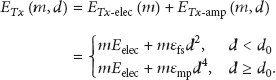
Among the three parts, wireless communication module plays the dominant role in the energy consumption. Many researches have been carried out on the low-energy radios. The first-order radio energy consumption model [25] is adopted for simulation. To transmit m-bit message over a distance d, the radio expends

$$\begin{array}{l}{E}_{Tx}\left(m,d\right)=E_{Tx\text{-elec}}\left(m\right)+E_{Tx\text{-amp}}(m,d)\\ \hspace{1em}\hspace{1em}\hspace{0.17em}\hspace{1em}=\{\begin{array}{ll}m{E}_{\text{elec}}+m{\epsilon }_{\text{fs}}{d}^{\mathrm{2}},\hfill & d<d_{\mathrm{0}}\hfill \\ m{E}_{\text{elec}}+m{\epsilon }_{\text{mp}}{d}^{\mathrm{4}},\hfill & d\ge d_{\mathrm{0}}.\hfill \end{array}\end{array}$$

(23)

To receive m-bit message, the radio expends

$$\begin{array}{cc}& E_{Rx}\left(m\right)=E_{Rx\text{-elec}}\left(m\right)=m{E}_{\text{elec}},\end{array}$$

(24)

where $E_{Tx\text{-elec}}$ and   $E_{Rx\text{-elec}}$ , separately denote the energy to activate the baseband circuits when transmitting and receiving. $E_{Tx\text{-amp}}$ is the energy to run the RF module. The electronic energy, $E_{\text{elec}}$ , denotes the energy spent to activate the baseband circuits to transmit or receive 1 bit. And ${\epsilon }_{\text{fs}}$ and   ${\epsilon }_{\text{mp}}$ denote the energy spent to run the RF module to transmit 1 bit in free space and multipath space separately. $d_0$ is a threshold indicating that if the distance is less than $d_0$ , the free-space model is used; otherwise, the multipath model is used. For the experiments, the communication energy parameters are set: $E_{\text{elec}}=50$  nJ/bit, ${\epsilon }_{\text{fs}}=10$  pJ/bit/m², and ${\epsilon }_{\text{mp}}=0.0013$  pJ/bit/m⁴.

From (23), we can derive $d_0$ as

$$\begin{array}{cc}& d_{\mathrm{0}}=\sqrt{\frac{{\epsilon }_{\text{fs}}}{{\epsilon }_{\text{mp}}}}=\mathrm{87.7}\hspace{0.17em}\text{m}.\end{array}$$

(25)

The packet is defined in Table 3.

Table 3

Packet descriptions.

Message type	Direction	Details	Length (bit)
CHInfoMesg	CH → node	8 + 16 + 32 + HEADER 8 → type, 16 → CH ID, 32 → coordinate	64
CHHandoverMesg (for GPF algorithm)	CH → CH	8 + 16 + 16 + 320 + HEADER 8 → type, 16 → previous CH ID, 16 → new CH ID, 320 → CH handover parameters (10 * 16 bits), including estimated target state and covariance	272
DataMesg	Node → CH	8 + 16 + 32 + 32 + 16 + HEADER 8 → type, 16 → node ID, 32 → node coordinate, 32 → measurement at time step $t_k$ , 16 → remaining energy	112
DataDegradeMesg	Node → CH	8 + 16 + 16 + HEADER 8 → type, 16 → node ID, 16 → node remaining energy	48
TargetToSinkMesg	CH → sink	8 + 16 + 64 + HEADER 8 → type, 16 → CH ID, 64 → target position estimation	96
TargetDegradeMesg	CH → sink	8 + 16 + HEADER 8 → type, 16 → CH ID	32
CHHandoverPFMesg (for PF algorithm)	CH → CH	8 + 16 + 16 + 43200 + HEADER 8 → type, 16 → previous CH ID, 16 → new CH ID, 43200 → CH handover parameters including 600 particles and weights	43248

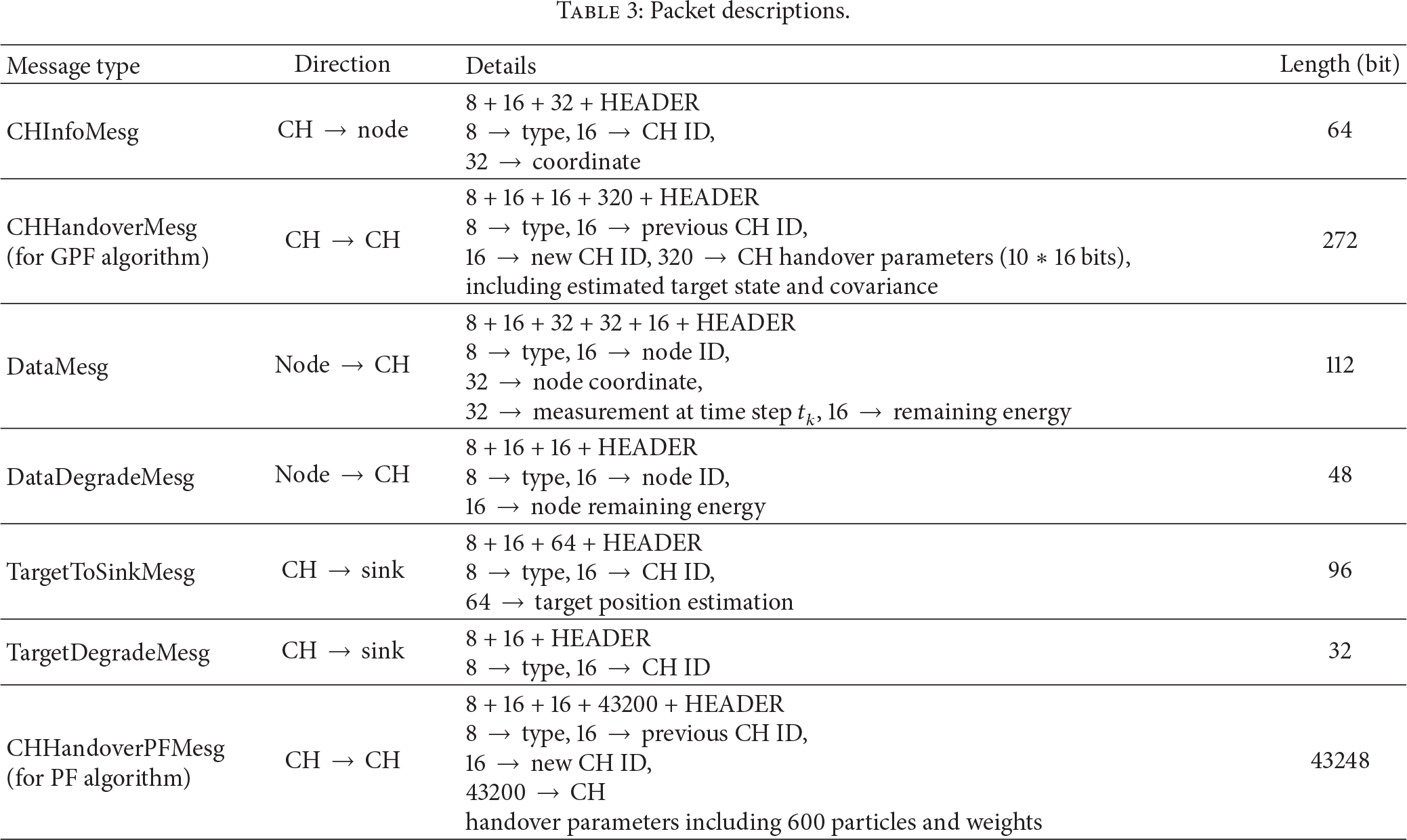
In all algorithms, the HEADER of the listed messages in Table 3 is 8 bits.

6. Simulation and Analysis

This section shows experimental studies for verifying the proposed framework.

6.1. Performance of Target Tracking

In order to demonstrate the GPF's satisfied performance of tracking accuracy, a comparison with PF [17] is carried out below. Here, we consider two cases: in PF-1, the mean and covariance for Gaussian noise are modeled precisely; the noise statistical parameters in PF-2 have large model error.

Figure 7 displays a typical trajectory and the tracking obtained by three different filtering algorithms. Figure 8 demonstrates the comparison of RMSEs of the estimated position and velocity obtained by three different filtering algorithms at each time step under 50 Monte Carlo runs ( $N_{\text{mc}}=50$ ).

Figure 7

Target tracking trajectory using GPF, PF1, and PF2 algorithm.

Figure 8

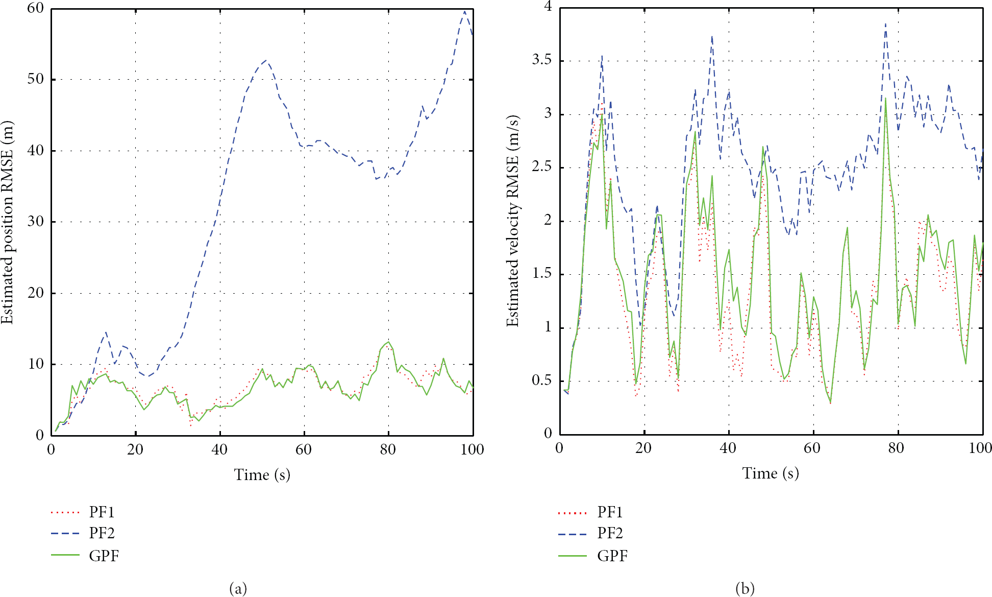
(a) The position RMSE. (b) The velocity RMSE.

As shown in Figures 7 and 8, we can see that the PF-1 algorithm has the best tracking accuracy, while PF-2 works badly. It is because that PF is greatly influenced by model parameters.

It is noted that the GPF algorithm outperforms the PF-2 with a close performance to PF-1 algorithm. Though GPF omits the resampling process, it preserves the desired accuracy of target estimation. Instead of handing over all particles to the new CH in a general PF algorithm, GPF only needs to transmit parameters (the mean and the covariance of the posterior distribution), which saves amount of energy. Further discussion will be detailed in Section 6.2.

To further validate the effectiveness of our proposed algorithm CSIFP, we compare it with those obtained from previous work [8, 11, 12], including CSIP1, CSIP2, and CSIP3 algorithms. All of them use GPF estimation method.

The tracking trajectories obtained by these algorithms are shown in Figure 9. Figure 10 demonstrates the average result of 50 Monte Carlo runs from up to down: (a) the RMSE in the estimated target position and (b) the RMSE in the estimated target velocity.

Figure 9

Target tracking trajectory using CSIP1, CSIP2, CSIP3, and CSIFP algorithm.

Figure 10

(a) The position RMSE. (b) Velocity RMSE.

It is clear that the tracking performance of CSIFP is comparable to the referenced methods (CSIP1, CSIP2, and CSIP3). CSIP1 performs best because of relying on the largest set of sensors' measurement. However, a rise in energy consumption appears. CSIP2 and CSIP3 approach a moderate precision due to their own strategies of CH selection and spatial fusion. It makes sense that the proposed CSIFP introduces not only spatial fusion but also time fusion, sacrificing the tracking accuracy in some degree. It is noteworthy that the slight performance degradation is worthy in contrast to the significant energy saving benefit in Section 6.2.

6.2. Performance of Network Energy Efficiency

In this subsection, we will firstly explain why the GPF algorithm is adopted by comparing generic PF's and GPF's energy consumption. Then the performance of energy efficiency in our proposed CSIFP is validated as well as the CSIP1, CSIP2, and CSIP3.

From Figure 11, the cumulative energy consumptions in PF-1 algorithm and PF-2 algorithm are nearly the same. It is obvious that energy consumption is uncorrelated with prior model of system noise. The GPF, by contrast, consumes least energy of the three. The theoretical proof is derived.

Figure 11

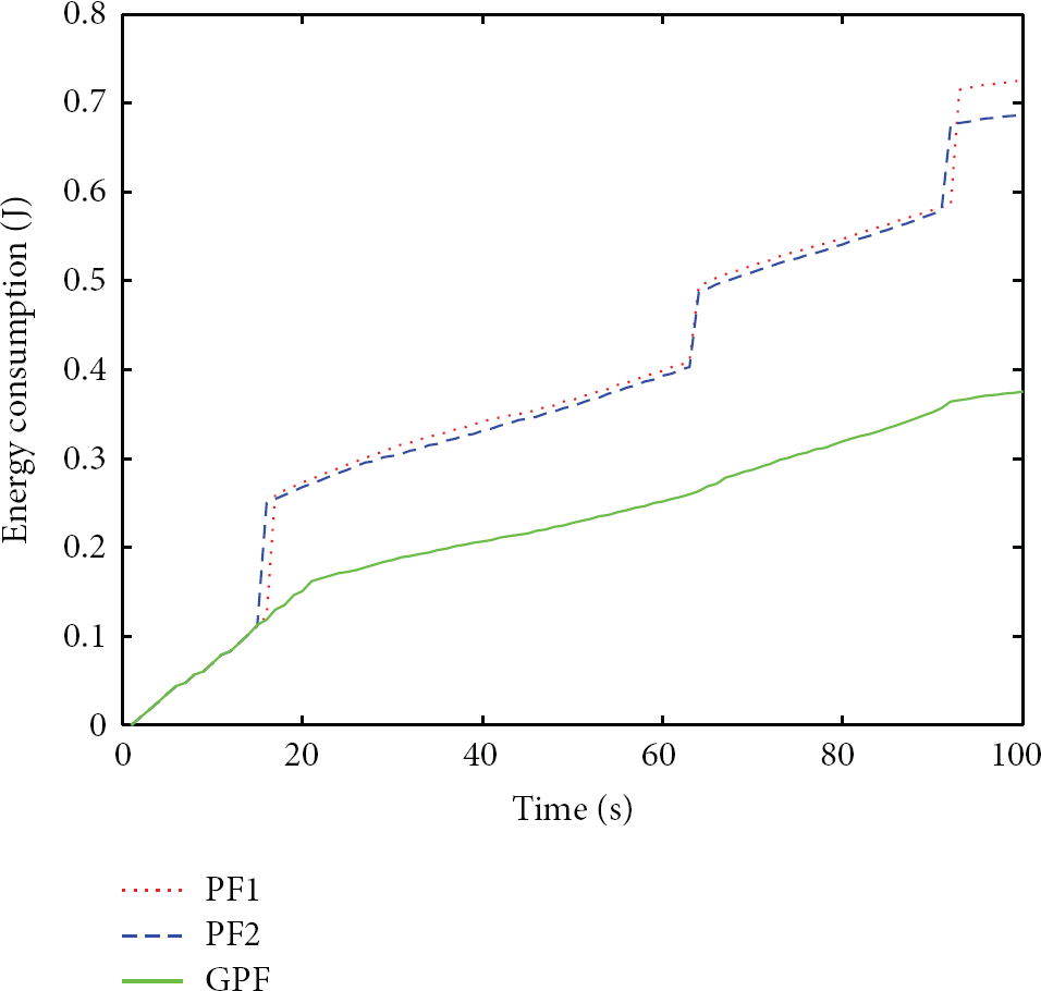
The cumulative communication energy consumption of PF and GPF after the entire tracking process.

In the PF algorithm, M particles and their weights are transferred when tracking task handover happens, and total quantity of data transmission is

$$\begin{array}{cc}& Q1=K·M+M,\end{array}$$

(26)

where K represents the dimension of the target state vector and $1\le K\le 6$ for the 2-D target tracking. M is the number of the particles, usually in the ${\mathrm{10}}^2$ order of magnitude or more. In the GPF algorithm, the current CH transmits nothing but the Gaussian mean and covariance of the target estimation. Considering the symmetry of the covariance, the quantity of the communication data is

$$\begin{array}{cc}& Q\mathrm{2}=K+K·\frac{\left(K+\mathrm{1}\right)}{\mathrm{2}}.\end{array}$$

(27)

It can be seen from Figure 12, the traffic of general PF algorithm is much bigger than GPF, and the latter's traffic has nothing to do with the particle number. The accuracy of the algorithm can be improved without a heavier traffic load by increasing the number of particles, if the computation complexity is accepted.

Figure 12

Traffic in different particle numbers and state dimensions for PF and GPF.

Figure 13 presents the total communication energy consumption of four different collaborative processing schemes. We can see that the CSIP1 consumes the most energy because all the active nodes with the $R_s$ range send their measurements to CH. The energy consumption of CSIP2 and CSIP3 is less than CSIP1 by choosing the candidate sensor nodes nearby the target to participate the tracking process. The former saves more energy due to selecting the farther member node as the new CH when CH changes, which reduces the handovers. The proposed CSIFP scheme consumes the least energy, because the CH selection method makes advantage of CSIP2, and the NNBA model is utilized to reduce the time redundancy as well. Consequently, the network payload approaches an expectable level.

Figure 13

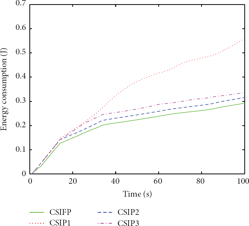
The cumulative communication energy consumption of CSIFP, CSIP1, CSIP2, and CSIP3 after the entire tracking process.

6.3. Performance of Robustness

Furthermore, for investigating the robustness of our proposed algorithm CSIFP, 6 independent Monte Carlo simulations with different trajectories are carried out. Figure 14 presents these random trajectories and tracking results obtained by these four algorithms. It is clear to us that CSIFP can keep good tracking accuracy when the trajectory changes.

Figure 14

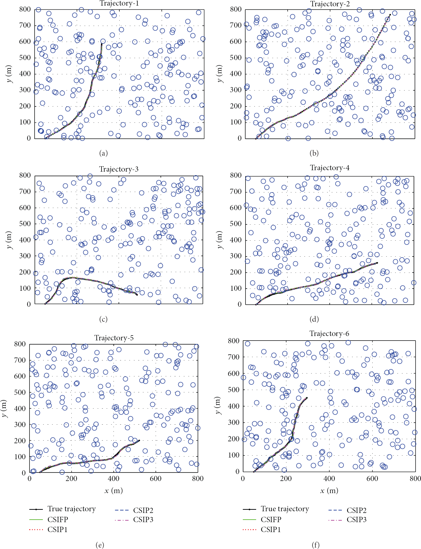
The performance of CSIP1, CSIP2, CSIP3, and CSIFP algorithm of 6 different trajectories.

To further verify the tracking performance of the proposed algorithm, the position RMSE and velocity RMSE are, respectively, illustrated in Figure 15 and Figure 16. The position RMSE curve of CSIFP has obvious fluctuation. It is because that CSIFP reduces time redundancy by NNBA model. NNBA model will be inertial if a slight shift happens in contrast to the previous measurement. Figure 17 demonstrates the total communication energy consumption of the tracking under four different collaborative processing schemes. We can see that CSIFP is energy efficient for it consumes the least amount of energy.

Figure 15

The position RMSE of 6 different trajectories.

Figure 16

The velocity RMSE of 6 different trajectories.

Figure 17

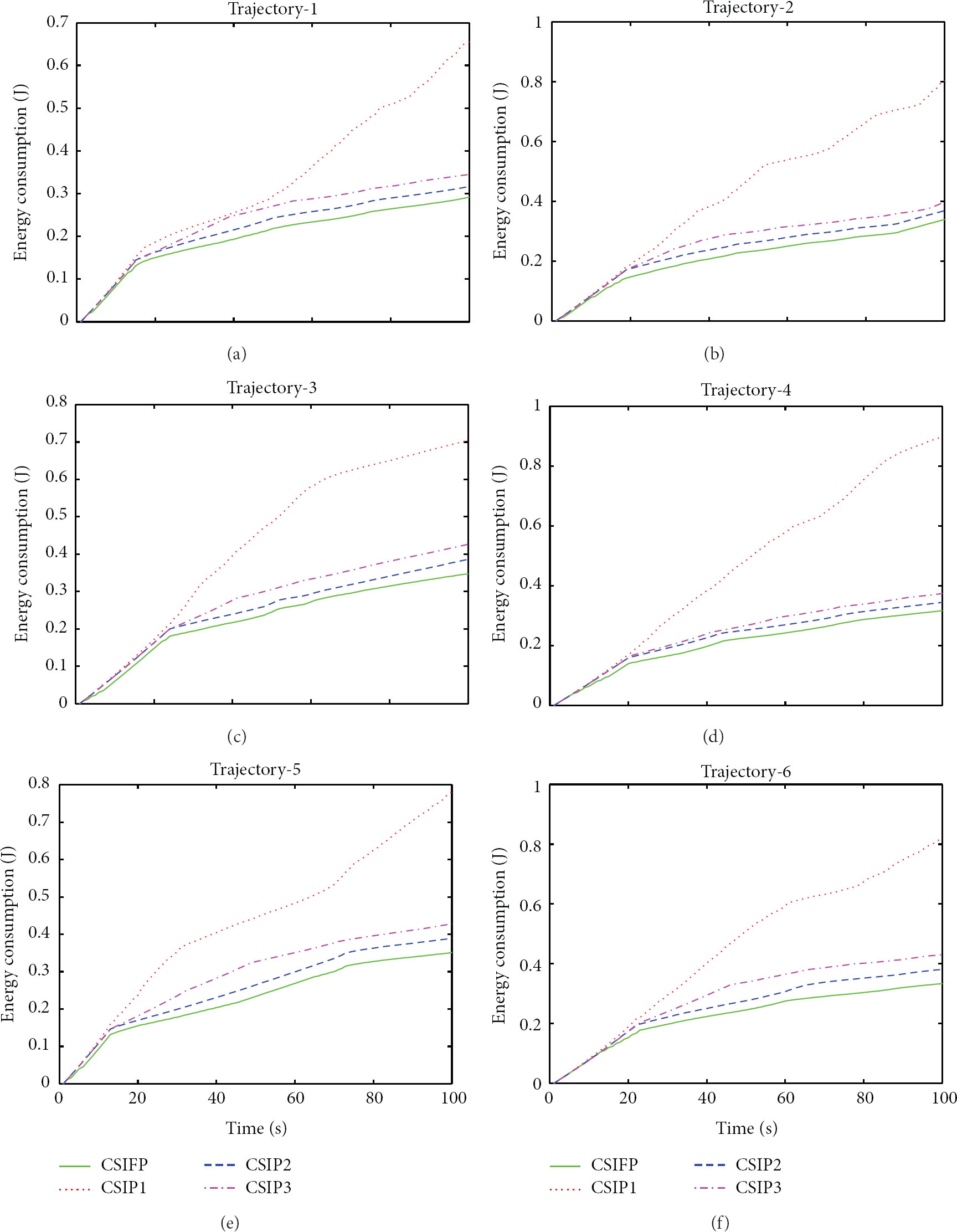
The cumulative communication energy consumption of CSIFP, CSIP1, CSIP2, and CSIP3 after the entire tracking process of 6 different trajectories.

Moreover, we carry out statistics by average RMSE and total energy consumption, as illustrated in Table 4. CSIFP achieves nearly the same good tracking accuracy. It obtains a gain of 56.83% in the energy cost in contrast with CSIP1, with a sacrifice of 12.88% in precision. Compared to CSIP2 and CSIP3, CSIFP consumes the least energy. This gain benefits from not only the CH selection method but also the fusion algorithm based on NNBA. From the above results, a good tradeoff between tracking accuracy and energy cost is achieved.

Table 4

Average result of performance.

	CSIFP	CSIP1	CSIP2	CSIP3
Position RMSE (m)	7.7646	6.9960	7.0706	7.3298
Velocity RMSE (m/s)	1.3077	1.4051	1.3125	1.2685
Energy cost (J)	0.3299	0.7775	0.3664	0.4001

7. Conclusions

In this paper, we have presented a high energy-effective strategy of collaborative signal and information fusion processing for acoustic target tracking applications in DWSNs. Within this framework, the whole network is assumed to be a neural network, in which the member nodes correspond to the neurons and the CH corresponds to the neural center. The nodes detect the target and transmit measurements to the CH. CH receives the information, responds to different neurons' stimulation, estimates the target state based on the GPF, and sends the estimation to the sink finally. Besides, a novel clustering scheme and CH selection method are implemented to balance the energy cost and tracking accuracy. The framework saves energy consumption through three aspects: (1) GPF algorithm transmits fewer but critical messages; (2) the NNBA model reduces the information redundancy; (3) the CH selection method demands less frequency of task handovers.

Last but not least, the numerical simulations directly validate that this collaborative tracking fusion framework can decrease the total network energy consumption and guarantee high tracking accuracy.

There have been several problems unresolved. Our proposed algorithm may not apply to the highly maneuverable case. The framework refers to the prior knowledge of the covariance matrices and noise variances, whereas they are usually unknown and time-varying in practical.