Self-Supervised Sensor Learning and Its Application: Building 3D Semantic Maps Using Terrain Classification

Abstract

An autonomous robot in an outdoor environment needs to recognize the surrounding environment to move to a desired location safely; that is, a map is needed to classify/perceive the terrain. This paper proposes a method that enables a robot to classify a terrain in various outdoor environments using terrain information that it recognizes without the assistance of a user; then, it creates a three-dimensional (3D) semantic map. The proposed self-supervised learning system stores data on the appearance of the ground data using image features extracted by observing the movement of humans and vehicles while the robot is stopped. It learns about the surrounding environment using a support vector machine with the stored data, which is divided into terrains where people or vehicles have moved and other regions. This makes it possible to learn which terrain an object can travel on using a self-supervised learning and image-processing methods. Then the robot can recognize the current environment and simultaneously build a 3D map using the RGB-D iterative closest point algorithm with a RGB-D sensor (Kinect). To complete the 3D semantic map, it adds semantic terrain information to the map.

1. Introduction

As seen in the Defense Advanced Research Projects Agency (DARPA) Grand Challenge, USA, robotics has progressed markedly from industrial robots that perform only given tasks to autonomous mobile robots that determine how to travel to a target. For robots to operate more intelligently, research on mobile robots needs to consider the following: (1) how to recognize certain objects, humans, or specific patterns; (2) simultaneous localization and mapping (SLAM) [1]; and (3) navigation to a specific destination. When an autonomous robot needs to reach a destination, the most important basic process before moving is for it to assess the safety of the surrounding environment and find a safe path for movement [2]. This process could incorporate global positioning system (GPS) and mapping technology, but a GPS system is not accurate enough to identify an exact position, and maps do not include all objects, especially moving objects. Therefore, a moving robot must be able to recognize the surrounding environment. One recognition method is terrain classification, in which a robot uses sensor responses to recognize the surrounding environment and determine possible safe pathways. This paper presents a method by which a robot equipped with a vision sensor can stop and classify terrain using self-supervised learning system and identify roads and sidewalks from passing vehicles and humans. Then it introduces the method used to create a three-dimensional (3D) map using a red/green/blue-depth (RGB-D) sensor (Kinect) and to add terrain information to create a 3D semantic map.

Figure 1(a) shows the environment of interest for this paper. It is an urban environment with a road for vehicles and a sidewalk for people. Figure 1(b) is the expected 3D semantic map after adding semantic information to the dense map.

Figure 1

(a) Example of an urban environment with a road, sidewalk, and buildings. (b) Example of a 3D semantic map (blue region: road; green region: sidewalk; red region: obstacles).

The remainder of this paper is organized as follows. We summarize related work in Section 2 and introduce the terrain-classification method and learning method for distinguishing between road and sidewalk through observations using a camera sensor in Section 3. Section 4 introduces the RGB-D iterative closest point (ICP) method, which uses a RGB-D sensor to make a 3D dense map and to develop a 3D semantic map by integrating the results of Section 3. Experimental results showing the effectiveness of the proposed method are presented in Section 5 and the conclusions and future research are presented in Section 6.

2. Related Works

2.1. Terrain Classification

During the past year, several studies have proposed methods for terrain classification. One study developed a method that involved searching for possible obstacles using a stereo camera, eliminating candidates based on texture and color clues, and then modeling terrain after obstacles had been defined [3]. Another study focused on avoiding trees in a forest; it used a stereo camera to recognize trees and classify terrain to find a safe pathway [4]. Other studies used a vibrating sensor to classify terrain that had already been traveled, based on various vibration frequencies [5].

However, these techniques only work in specific environments. Robots need to be able to learn about unknown terrain. Some studies have focused on supervised learning that requires human intervention when a robot reaches an unknown area. Due to the limitations of supervised learning, many researchers are now working on self-supervised or unsupervised techniques, in which a robot can learn about an environment on its own, without any human supervision.

One recent study developed a technique in which a robot can calculate the depth of a ground plane using a depth map generated by a stereo camera and can classify and learn about the ground and obstacles within 12 m. Based on these data, it can recognize very distant regions, as far as 30–40 m [6]. Another study developed an unsupervised learning method that deletes incorrect detections about a wide variety of terrain types (e.g., trees, rocks, tall grass, bushes, and logs) while the robot navigates and collects data [7]. Yet another study involved self-supervised classification using two classifiers: an offline classifier that used vibration frequencies to provide the other classifier, an online and visual classifier, with labels for various observed terrains. This allowed the visual classifier to learn about, and recognize, new environments [8].

However, some of these methods require more than one sensor; some use stereo cameras or vibrating sensors with monocular cameras, and most assume either that the robot is facing a flat plane through which it can navigate or that the robot will learn about the terrain after it navigates through it.

2.2. 3D Map Building

The construction of 3D maps using various sensors has been studied, including range scanners [9], stereo cameras [10], and single cameras. The biggest problem in constructing a 3D map is the alignment of captured images. To process 3D laser data, the ICP algorithm is widely used [9]. This algorithm finds a rigid transformation of the optimal distance between a point on the frame and each other point on the frame repeatedly. A passive stereo image system can extract depth data for features through the paired images. The feature points may be combined via optimization similar to the iterative process of the first ICP. Then, additional algorithms such as the random sample consensus (RANSAC) algorithm can be used to solve the problem of consistency [10].

Recent research on creating 3D maps has obtained depth information for each pixel using a sensor that simultaneously extracts a color depth image and a general video, such as by combining Kinect with a time-of-flight (TOF) camera [11]. Kim et al. [12] built a 3D map using a fixed TOF camera that had a frame unrelated to the order of time. In contrast, Henry et al. [11] proposed a 3D map-building method that used a freely moving RGB-D sensor and information on time, shape, and appearance simultaneously.

3. Self-Supervised Terrain Classification

The proposed method is based on a self-supervised framework. The robot observes moving objects and determines their movement along roads and sidewalks. From these data it extracts image data (e.g., patch) about the terrain and classifies it as one of three classes (road, sidewalk, or background). This framework consists of three parts: detection and tracking of moving objects, recognition of paths taken by moving objects, and learning the terrain patches that were extracted from the paths taken by moving objects and classifying the environment.

The proposed method has two classifiers. One is for classifying moving objects; this is offline and supervised learning. The other is for classifying terrain; this is self-supervised learning, and it also learns image patches, based on labels generated by the object classifier. Both classifiers are Support Vector Machines (SVM) as proposed by Vapnik [13] and both use only visual features.

3.1. Detection and Tracking of Moving Objects

For this study, we assumed that only humans and vehicles move in the outdoor environment. Thus, moving objects are defined in two classes: human and vehicle. Background subtraction is used to detect moving objects; this involves a mixture of adaptive Gaussians [14]. The system tracks objects based on their size and location. Figure 2 shows the results of detection, classification, and tracking of moving objects.

Figure 2

Detection, classification, and tracking of moving objects ((a) the result of background subtraction, (b) the result of object classification (blue square: human, green: vehicle) and tracking based on size and location).

3.2. Object Classification

To identify whether a detected object is human or vehicle, the SVM selects an object classifier. Data about the object's edge are used for a feature vector. This classifier also provides information about what class of terrain is involved.

( 1) Classifier. The first SVM in this system classifies objects as either human or vehicle. This binary classification can be expressed as (1) where the classification function is $f:{\Re }^n\to \pm \mathrm{1}$ , $x_i$ is a training vector, and $y_i$ is a label of class. For example, $x_i$ is an object's edge feature vector and $y_i$ shows that a positive object is classified as human and a negative object is classified as vehicle:

$$\begin{array}{cc}& f\left(x\right)={{\displaystyle \sum }}_{i=\mathrm{1}}^N{y}_i{\alpha }_{i}k\left(x,x_i\right)+d,\end{array}$$

(1)

where N is the number of total training data and $k()$ is a kernel function and we used the Radial Basis Function (RBF) which is $k(x,x_i)=e^{-\parallel x-x_i\parallel /\mathrm{2}{\sigma }^{\mathrm{2}}}$ as the kernel function. ${\alpha }_i$ and d are weights that reduce numbers of wrong classification by making a distance between a hyper plane and support vectors far and these weights are calculated by changing to an optimized problem using

$$\begin{array}{l}\max \hspace{0.17em}{L}_D\equiv {{\displaystyle \sum }}_{i=\mathrm{1}}^N{\alpha }_i-\frac{\mathrm{1}}{\mathrm{2}}{{\displaystyle \sum }}_{i=\mathrm{1}}^N{{\displaystyle \sum }}_{j=\mathrm{1}}^N{y}_i{y}_j{\alpha }_i{\alpha }_{j}k\left(x_i,x_j\right)\\ \text{subject}\hspace{0.17em}\text{to}\hspace{0.17em}\hspace{0.17em}{{\displaystyle \sum }}_{i=\mathrm{1}}^N{y}_i{\alpha }_i=\mathrm{0},\hspace{1em}\mathrm{0}\le {\alpha }_i\le C,\end{array}$$

(2)

where C is a constant to minimize incorrect classification and d is calculated with ${\alpha }_i$ and support vector using (1) [15, 16]. This SVM is implemented using LIBSVM [17, 18].

( 2) Features. The feature vector for the object classifier is a global edge histogram of the object's region [19, 20]; this is shown in (3) and also consists of responses from four orientations and other data:

$$\begin{array}{cc}& G_o=\left[g_o^v,g_o^h,g_o^{\mathrm{45}},g_o^{\mathrm{135}},g_o^n\right],\end{array}$$

(3)

where $G_o$ is a feature vector of edge responses of an object, o is the region of an object, $g_o^v$ expresses the response about the vertical orientation of object's region, $g_o^h$ is for horizontal, $g_o^{\mathrm{45}}$ is for 45°, $g_o^{\mathrm{135}}$ is for 135°, and $g_o^n$ is the response about nonedges. These feature values are normalized 0 to 1.

3.3. Data Association and Path Extraction

To extract human and vehicle movement paths (see Figure 3), the system saves data about objects $O_k$ at every frame during the classification and tracking of moving objects, in which k means the kth appearance of a moving object during the observation. These data include the kth object's locations in terms of image coordinate $X_k$ and volume $V_k$ (which consists of the object's width $w_k$ and height $h_k$ ); the number $i_k$ times the kth object is tracked and the accumulated label value $l_k$ that is generated by classification. These data are shown as follows:

$$\begin{array}{l}{O}_k\supset \left(X_k\cup V_k\cup \left\{i_k,l_k\right\}\right),\\ X_k=\left\{{\left(x,y\right)}_{k,\mathrm{1}},{\left(x,y\right)}_{k,\mathrm{2}},\dots ,{\left(x,y\right)}_{k,i_k}\right\},\\ V_k=\left\{w_k,h_k\right\},\\ \phantom{hhhhhhhhhhhhhhhhh}\left(k=\mathrm{1,2},\dots ,K\right).\end{array}$$

(4)

Figure 3

Path extraction about moving objects and lines shows its path (blue: human, green: vehicles).

Here, K is the number of total objects that are detected as moving object; our system defines the bottom-left of the image as zero in the image coordinates. Algorithm 1 shows the entire process of data collection and association about a moving object.

Algorithm 1: Data collection and association.

(1) Observe the object that is moving ( $O_n$ is the object is detected at this frame).

(2) Confirm whether the presently detected object $O_n$ was seen before or not by comparing it with

   every object $O_k$ that was already detected, based on size and position data of the objects $O_k$ .

  (2a) If the object $O_n$ was seen before (e.g., $V_n$ and $(x,y{)}_{n,\mathrm{1}}$ are similar to $V_k$ and $(x,y{)}_{k,i_k}$ ),

    update data of $O_k$ through $X_k\leftarrow X_k\cup \{(x,y{)}_{n,\mathrm{1}}\}$ , $V_k=\{w_n,h_n\}$ , $i_k=i_k+\mathrm{1}$ and $l_k=l_k+l_n$ .

  (2b) If the object $O_n$ is seen for the first time, create new object data $O_{k+\mathrm{1}}$ same as $O_n$ .

     Thus, the total number of detection objects K increases to $K+\mathrm{1}$ .

(3) Check whether K is a multiple of β.

  (3a) If it is, do path extraction.

  (3b) If it is not, keep observing until K becomes the next multiples of $\mathrm{\beta }$ .

Algorithm 1 ( $2\text{a}$ ) shows that elements of location data $X_k$ increase by $(x,y{)}_{n,\mathrm{1}}$ as $(x,y{)}_{k,i_{k+\mathrm{1}}}$ , the object's volume $V_k$ is replaced by $\{w_n,h_n\}$ , the number of iterative tracking $i_k$ is increased by one and labeled with the value $l_k$ , which shows the class of the object, accumulated by the classification results of the newly detected object $l_n$ .

We can use data about moving objects $O_k$ to identify movement paths, in which sidewalk S and road R are a set of image coordinates. Algorithm 1 (3) presents how and when data are sufficient for the system to extract a path. Here, $\beta =\mathrm{5}$ , which means that path extraction proceeds each time an object is observed over multiple $\beta (=\mathrm{5})$ observations. Algorithm 2 shows the process of path extraction in pseudocode.

Algorithm 2: Path extraction.

$\mathrm{K}$ = The total number of detected objects

$\mathrm{T}$ = The threshold for defining a moving object

Sidewalk map: A map that includes the total paths of human movement

Road map: A map that includes the total paths of vehicle movement

Input: All detect object $O_k$    $(\mathrm{k}=\mathrm{1,2},\dots ,\mathrm{K})$

Goal: Find all paths on which humans and vehicles move (Sidewalk: S, Road: R)

(0) Initialize S, R, Sidewalk map and Road map

(1) for   $k=\mathrm{1}$ to K do

(2) if $i_k\ge T$ then

(3)   $O_k$ is a moving object

(4)  for $i=\mathrm{1}$ to $i_k$ do

(5)    $x_{k,i}^{\prime }=x_{k,i}-h_{k,i}/2$

(6)  end for

(7)  if $l_k>0$ then

(8)  for $i=\mathrm{1}$ to $\left(i_k-1\right)$ do

(9)   Draw a line from ${(x^{\prime },\mathrm{y})}_{k,i}$ to ${(x^{\prime },\mathrm{y})}_{k,i+1}$ into Sidewalk map

(10)    end for

(11) else

(12)  for $i=\mathrm{1}$ to $(i_k-\mathrm{1})$ do

(13)   Draw a line from ${\left(x^{\prime },\mathrm{y}\right)}_{k,i}$ to ${\left(x^{\prime },\mathrm{y}\right)}_{k,i+1}$ into Road map

(14)  end for

(15) else

(16)   $O_k$ is a noise

(17) end for

(18) for all pixels of Sidewalk and Road map do

(19) if Sidewalk $\left(x,y\right)\text{!}=\mathrm{0}$ then $S\leftarrow S\cup \left\{\left(x,y\right)\right\}$

(20) if Road $\left(x,y\right)\text{!}=\mathrm{0}$ then $R\leftarrow R\cup \left\{\left(x,y\right)\right\}$

(21) end for

In Algorithm 2, lines (2), (3), (15), and (16) show how observed objects are defined as useful or not, based on the assumption that the object is observed over a certain number of iterative frames $T(=30)$ with a specified number of iterative tracking $i_k$ . Line (5) shows that the x-coordinates of the bottom of the object are the path's x-coordinates, and the path's y-coordinates are the same as the object's y-coordinates. Lines (7) and (11) show whether the observed object over a certain number of iterative frames is a human or a vehicle based on its accumulated label value $l_k$ : when $l_k$ is positive, the object is a human; when $l_k$ is negative, the object is a vehicle. Lines (18)–(21) show how the system obtains path data S and R based on a $Sidewalk$ map and a $Road$ map (cf. $Sidewalk(x,y)$ refers to the intensity of the map at image coordinates $(x,y)$ : it is not zero when one point of lines appears at these coordinates).

Additionally, we use maps, which are one-channel image spaces, to save object's movements and conduct random sampling for patches based on path data generated from maps. If we used raw position data instead of path data, patch sampling would be very dependent on the object's location, rather than random, because objects appear at similar locations in an image when it is located over the camera's focal length. We can solve this problem by drawing lines onto maps and using these to generate path data. The elements of both path data should be more than $\delta \times 0.4$ , where δ is the length of the image diagonal. If it is not, the system returns to the observation step.

3.4. Terrain Data Extraction

Terrain data about sidewalks and roads are randomly extracted from each path S and R.

Then to extract nonpathway regions (cf., in this study, these regions were defined as backgrounds) not only means that ${\mu }_{q,j}$ and standard deviations ${\sigma }_{q,j}$ of feature values (see (8)) of each sidewalk and road are calculated but also that candidates of backgrounds are extracted using global random sampling. Here, q is an index of terrains which expresses either the sidewalk (i.e., S) or the road (i.e., R) and j is an index which means jth feature; range of j is 1 to D and D stands for dimensions of the feature vector (i.e., 11). The candidates of backgrounds are clustered using Mean-Shift algorithm [21] and $\mathrm{mod}{e}_{e,j}$ denotes jth features’ mode of eth cluster.

And eth cluster of backgrounds candidates is selected as backgrounds data; that is, $\text{B}{\text{G}}_e=\mathrm{1}$ , when a gap $\text{Ga}{\text{p}}_{q,e}$ between the mode of the cluster and the mean of the extracted sidewalks and roads data is larger than a distance $\text{Dis}{\text{t}}_q$ which can be calculated using standard deviations ${\sigma }_{q,j}$ (see Figure 4):

$$\begin{array}{cc}& \text{Ga}{\text{p}}_{q,e}=\sqrt{{{\displaystyle \sum }}_{j=\mathrm{1}}^D{\left(\mathrm{mod}{e}_{e,j}-{\mu }_{q,j}\right)}^{\mathrm{2}}},\end{array}$$

(5)

$$\begin{array}{cc}& \text{Dis}{\text{t}}_q=\lambda \sqrt{{{\displaystyle \sum }}_{j=\mathrm{1}}^D{\left(n·{\sigma }_{q,j}\right)}^{\mathrm{2}}},\end{array}$$

(6)

$$\begin{array}{cc}& \text{B}{\text{G}}_e=\{\begin{array}{cc}1\hfill & \text{if}\hspace{0.17em}\hspace{0.17em}\text{Ga}{\text{p}}_{S,e}>\text{Dis}{\text{t}}_S,\hspace{0.17em}\hspace{0.17em}\text{Ga}{\text{p}}_{R,e}>\text{Dis}{\text{t}}_R\hfill \\ 0\hfill & \text{else}.\hfill \end{array}\end{array}$$

(7)

Figure 4

Example of 2D features clustering, and comparisons of clusters with sidewalks and roads data. Deep blue: a distribution of the sidewalk data, deep red: a distribution of the road data, small dots: candidates of the background; same color represents same cluster.

In this study, we assumed that distributions of extracted sidewalks and roads data were the Gaussian distributions. Thus, n in (6) is a multiple of the standard deviation that specifies the width of the interval (i.e., $n=1$ : 68%, 2: 95%, 3: 99.7% confidence intervals) and is set at 2. λ is a weight which influences a distance and is calculated by 95% confidence intervals, and also it is set at 2.

Figure 4 shows an example of 2D features clustering and notations.

The size of terrain data, that is, patch size, is set at $12*12$ ; the numbers of extraction are set at 200 for sidewalk and road classes and 400 for the background class, based on experimental results about classification performance using various numbers of training data.

Figure 5 shows experiments about backgrounds candidates clustering in which clusters were selected as background or not.

Figure 5

(a) The result of clustering (small dots: candidates of the background; same color represents same cluster), (b) the result of terrain data extraction (red dots: background, blue dots: sidewalk, green dots: road, the others: excluded clusters of candidates from background class).

3.5. Terrain Classification

The terrain classifier learns terrain data generated using observed paths as a feature vector (see (8)) and determines where a robot can move within the surrounding environment as a self-supervised learning method. For a case with different numbers of training data, we can weigh each terrain class according to the number of data in its own class compared with the total number of data in all classes. The use of features and classifiers to classify image data into class labels has been popular in recent years [22].

( 1) Classifier. We defined terrain using three classes (sidewalk, road, and background) and used a multiclass SVM for terrain classification.

SVM systems were initially designed for binary classification, but two common methods allow SVM systems to classify more than two classes: one method involves combining numerous binary SVM systems. The other involves approaching a problem as an optimization problem and considers all data simultaneously.

We selected the former approach, specifically the one-against-one method. It constructs ${\mathrm{\hspace{0.17em}\hspace{0.17em}}}_k{C}_{\mathrm{2}}=k(k-\mathrm{1})/\mathrm{2}$ as a classifier to define k-classes and then uses MaxWins, a voting system, to predict a final class with the most votes [23].

( 2) Features. We used two visual features, color and texture, for the terrain classifier. We used RGB and Lab color spaces for color features; these have been proven as good features for scene classification [24] and we used a Global Edge Histogram for texture features. Equation (8) presents the visual feature vector used for the terrain classifier:

$$\begin{array}{cc}& F_p=\left[R_p,G_p,B_p,L_p,a_p,b_p,f_p^v,f_p^h,f_p^{\mathrm{45}},f_p^{\mathrm{135}},f_p^{\text{non}}\right],\end{array}$$

(8)

where $F_i$ is a feature vector of the image patch (e.g., p). $R_p$ , $G_p$ , $B_p$ , $L_p$ , $a_p$ , and $b_p$ are mean values of each channel of RGB and Lab color. $f_p^v$ expresses the response for a vertical orientation of the patch, $f_p^h$ is for horizontal, $f_p^{\mathrm{45}}$ is for 45°, $f_p^{\mathrm{135}}$ is for 135°, and $f_p^{\text{non}}$ is the response for nonedges. These feature values are normalized 0 to 1.

4. 3D Semantic Map Building

This paper constructs a 3D semantic map that shows regions where people or vehicles can move. To build the 3D map, it is necessary to determine the position of the sensor at every time point. It is possible to estimate the location with the sensor or to do so more precisely using multiple sensors. Normal position estimation can use the motion model of the robot and it is also possible to make use of GPS or an image process. We build the 3D map using the position of the robot estimated by matching the point cloud and features from the image and odometry data.

4.1. Ground Plane Estimation with Vertical Disparity Map

Using a learning environment based on the trajectories of passing vehicles and humans, it is still possible to classify some terrains incorrectly because their texture and color differ completely. For example, as shown in Figure 6(a), the sidewalk might be recognized as an obstacle because there are so many leaves with different colors and textures on it. However, we can assume that a sidewalk or road is in the same plane after obtaining the ground plane. Then, we solve this drawback by depending on the class that forms the principal of the plane.

Figure 6

(a) A sidewalk with complex texture, such as fallen leaves. (b) The road plan estimated using a V-disparity map.

To estimate the plane, V-disparity is widely used to detect obstacles and the plane [25]. The horizontal axis of the V-disparity map indicates the depth, and the vertical axis is made by accumulating the pixels with the same depth along the horizontal axis of the depth data. A plane in the 3D world actually appears in the form of a line in the V-disparity map. Therefore, the extraction of a strong line from the V-disparity map represents the ground plane. Extraction of the ground plane is shown in Figure 6(b). The ground plane is determined using the voting method “Max Wins” to obtain the most votes from parts of the terrain class for planes. A value exceeding the plane in the column direction in a V-disparity map is an obstacle [26].

4.2. Map Building Using RGBD Iterative Closest Point

The ICP algorithm searches for the rigid transformation that minimizes the distance between the source point cloud, $P_s$ , and the target point cloud, $P_t$ . The process repeats the optimization and alignment of the cloud data until convergence. The ICP algorithm is useful when some extent of the adjustment point cloud of two points is aligned. Conversely, when the data association between the point clouds of two points is not accurate, a local minimum occurs, which is inappropriate convergence [11]. In contrast, visual alignment makes use of feature point matching. The main advantage of using visual features is that it does not require an initialization process and can be corrected using the RANSAC algorithm. However, due to the inaccuracy of the scale, two-dimensional (2D) matching does not guarantee an optimal solution.

In this paper, we apply the RGB-D ICP algorithm, which has the advantage of matching RGB-D data in two ways. The algorithm is described in Algorithm 3. It takes input source $P_s$ and target $P_t$ from the RGB-D sensor to obtain a rigid transformation of the camera. Lines (1) and (2) in Algorithm 3 describe the extraction of visual features and association between $P_s$ and $P_t$ . We use the Harris corner point as the visual feature. To calculate the optimal-rigid transformation $t^{*}$ between two feature point sets, the RANSAC algorithm is applied in line (3). Perform_RANSAC_Alignment searches for the transformation of the best alignment by matching sets and selecting the features of three points repeatedly. Then the number of inliers is counted for the remaining feature points. The transformation is estimated with most pairs of the inlier. The association $A_f$ with matched feature points is also determined through the transformation.

Algorithm 3: RGBD-ICP algorithm.

(0) $F_{source}$ = Extract_RGB_point_features( $P_s$ )

(1) $F_{target}$ = Extract_RGB_point_features( $P_t$ )

(2) ( $t^{*}$ , $A_f$ ) = Perform_RANSAC_Alignment( $F_{source}$ , $F_{target}$ )

(3) repeat

(4)   $A_d$ = Compute_Closet_Points( $t^{*}$ , $P_s$ , $P_t$ )

(5)   $t^{*}={\underset{t}{\text{argmin}}}_{}\mathrm{\alpha }\left(\frac{1}{\left|A_f\right|}{\displaystyle \sum }_{i\in A_f}{w_i\left|t\left(f_s^i\right)-f_t^i\right|}^2\right)+\left(1-\alpha \right)\left(\frac{1}{\left|A_d\right|}{\displaystyle \sum }_{j\in A_d}{w_j\left|(t\left(p_s^j-p_t^i\right)·n_t^j\right|}^2\right)$

(6) until (Error_Change $(t^{*})\le \mathrm{\theta }$ ) or (maxIter reached)

(7) return   $t^{*}$

Lines (3) to (6) are the main loop of the ICP algorithm. The association $A_d$ between point clouds is calculated at line (4). This process converts the source point cloud $P_s$ using transformation t. Then the first initialization is done with a visual RANSAC transformation. Consequently, it is possible to match the point cloud without knowing the relative orientation of clouds. Line (5) minimizes the alignment error of the point cloud association and the visual feature matching between clouds. The first term of the error function represents the average distance of the association of visual features and the second indicates the error distance of the association between clouds. Finally, we give the two errors a weight of a. The process ends when any errors have been reduced sufficiently or the maximum number of iterations, which was predetermined, is reached. It determines the ICP transformation using the odometry data of the robot, when RANSAC does not find sufficient inliers.

Figure 7 shows a 3D map created using the RGB-D ICP algorithm in an outdoor environment. This map will become a 3D semantic map when the results of terrain classification are added.

Figure 7

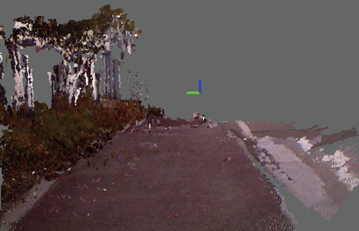
An example of a 3D map using the RGB-D ICP algorithm.

5. Experiments

5.1. Experimental Environment

We conducted experiments at four locations at Seongdong-gu, Seoul, Republic of Korea, and captured test datasets using a camera set at $640*360$ .

The experiments involved a robot observing moving objects and learning about the surrounding terrain based on the paths of moving objects; the robot was motionless with the assumption that it was in an unknown location.

To extract a reasonable number of patches, test was conducted to classify terrain with various numbers of training data. Figure 8 presents the results.

Figure 8

Classification performance with various numbers of training data in whole dataset.

We evaluated the proposed method by comparing its results with those of supervised learning, which ensured correct labels using ground-true images. Both methods randomly extracted training data about each terrain (sidewalk: 200, road: 200, background: 400) based on Figure 9. To train the object classifier, which involves offline learning, about 1968 units of training data were obtained from NICTA [27] and UIUC [28]. Each class of object (i.e., humans and vehicles) had the same amount of data; the RBF kernel parameter γ, which was used for training, was ${\mathrm{2}}^{-\mathrm{3.5}}$ and it was generated using a tool provided by LIBSVM [17]. The performance of the object classifier was 94.5408% based on 10-fold cross-validation, which was also provided by the LIBSVM tool.

Figure 9

Experimental results. Columns present the results and processes of experiments in the whole dataset. (a) Experimental environments, (b) extraction of training patches based on paths after observing moving objects, (c) ground-true images for terrain classification (red: background, green: road, blue: sidewalk), (d) supervised terrain classifications based on ground-true image, (e) classification results of the proposed method.

5.2. Results of Self-Supervised Terrain Classification

In this study, self-supervised classification was compared to supervised classification, and classification error rates for both methods were compared with ground-true images. Table 1 lists the terrain classification error rates as mean and standard deviation in four datasets. Tests were conducted 10 times for extraction patches, training, and classification for each dataset.

Table 1

Comparison of self-supervised classification and the supervised learning method.

Dataset	Mean error rate (STD DEV)
	Supervised classification	Self-supervised classification
1	4.58% (0.32%)	8.79% (1.14%)
2	5.23% (0.29%)	14.39% (0.56%)
3	3.30% (0.73%)	6.08% (0.36%)
4	8.00% (0.24%)	17.11% (1.41%)

Table 1 shows that the results of the proposed method were approximately 3–9% different to those of supervised classification. The biggest difference between supervised and proposed classification result was 11% in dataset 2. As shown in Figure 9, the most wrong classification appeared in boundaries between roads and sidewalks, because any human or vehicles did not pass through these regions and also those had different color and textures compared to sidewalk and road. This fact could be found in datasets 3, 4, and 1 which turned out the second, third, and fourth worse classification results. To sum up, the performance of the proposed method might be almost the same as the supervised method which was conducted by human interventions who expects the problem that critically happened at dataset 2, such as the boundary regions.

Figure 9 presents the experimental environments, extraction of patches for terrain classes based on the paths of moving objects, ground-true images of terrain, supervised terrain classification, and the results of the proposed method per dataset.

5.3. Results of 3D Map Building with Terrain Classification

After self-supervised learning by observing objects moving in the unknown environment, the robot moves around to build a 3D map with the RGB-D sensor. The result is shown in Figure 10. Finally, Figure 11 shows a 3D semantic map that includes the result of the terrain classification. Compared to Figure 10, the map was created by classifying terrain regions as road, sidewalk, and obstacles that the robot cannot move through, such as trees and buildings. However, the proposed terrain classification has a disadvantage in that the region between the sidewalk and road is classified as an obstacle that the robot cannot pass through.

Figure 10

(a) 3D map of the university, (b) RGB images of the same scene.

Figure 11

(a) The 3D semantic map. (b) Magnification of part of the 3D semantic map (red: obstacles; blue: road; green: sidewalk).

6. Conclusions

We proposed a self-supervised terrain classification framework in which a robot observes moving objects and learns about its environment based on the paths of the moving objects captured using a monocular camera. The results were similar (ca. 3–9% worse) to those of supervised terrain classification methods, which is sufficient for an autonomous robot to recognize its environment. In addition, we built a 3D dense map with a RGB-D sensor using the ICP algorithm. Finally, the 3D semantic map was created by adding the results of the terrain classification to the 3D map.

In future research, we will focus on better ways to extract background data, using a vanishing point or depth data and a total framework for navigation. We will also conduct tests in various environments, such as indoors and unstructured outdoor environments.