Higher Order Variational Integrators for Multibody System Dynamics with Constraints

Abstract

The continuous and discrete Euler-Lagrangian equations with holonomic constraints are presented based on continuous and discrete Hamiltonian Principle. Using Lagrangian polynomial to interpolate state variables and Gauss quadrature formula to approximate Hamiltonian action integral, the higher order variational Galerkin integrators for multibody system dynamics with constraints and the computation procedure are given. Numerical examples are provided to show the long-time behavior of the methods proposed in this paper via comparisons with traditional Runge-Kutta methods.

1. Introduction

Dynamics of multibody systems [1] are usually described by a set of differential-algebraic equations (DAEs) [2, 3], which are solved traditionally using numerical methods of ordinary differential equations (ODEs) and combining some constraint stabilization techniques. In the community of numerical analysis, numerical methods for ODEs are always designed in a small area with local stability analysis, which lead to a lot of difficulties for long-time simulation. Geometric numerical integration methods [3] originated from long-term simulation of molecular dynamics and planet dynamics in solar system with global numerical stability due to the property of structure-preserving provide alternatives to overcome these problems. These numerical methods are referred to as the ones preserving the invariants in their corresponding continuous systems, such as preserving symplectic, energy, momentum, symmetry, and orthogonality, in the original systems, thus revolutionizing the traditional concepts of numerical stability. It has been widely accepted that the more invariants conserved in a numerical method, the more stable it is.

Symplectic algorithms [4] and energy conservation methods [5] are two frequently used methods for numerical integration of constrained Hamiltonian systems, but they are designed for conservative systems and it is difficult to design an algorithm that is symplectic and energy preserving at the same time [6]. The variational integrators [7, 8] based on discrete variational principle [9] provides an excellent framework for design of geometric numerical integrators with many merits: it preserves momentum naturally with good behavior of approximate energy conservation, even preserves strictly symplectic-momentum-energy [10]; it can be easily extended to a large class of problems [11, 12], such as the construction of geometric structure-preserving numerical integrators for PDEs [13], nonsmooth collisions [14, 15], stochastic systems [16, 17], nonholonomic systems [18, 19], and constrained systems [20], dissipative systems [21], optimal control [22, 23], parameter optimization [24]; it can generate easily a large class of higher order methods based on polynomial interpolation and numerical quadrature formulas systematically [25–29] and some Lie group variational integrators [30–32] combining Lie group methods [33].

For the general conservative systems without constraints, [25, 26] propose the same framework of design higher order variational Galerkin integrators using numerical interpolation and quadrature techniques for state variables and action integral, respectively, during one integration step based on discrete variational principle. Motivated by these works, we will investigate higher order variational Galerkin integrators for multibody system dynamics with constraints for the long-term simulation purpose. Due to the space limit, we will focus on the cases with holonomic constraints, but the results can be easily extended to the cases with nonholonomic constraints and the cases with nonconservative forces.

The paper is organized as follows. In Section 2, the continuous and discrete Euler-Lagrangian equations with holonomic constraints are presented based on continuous and discrete Hamiltonian Principle, respectively; in Section 3, we derive the higher order variational Galerkin integrators for multibody system dynamics with constraints using Lagrangian polynomial to interpolate state variables and using Gauss quadrature formula to approximate Hamiltonian action integral; the computation procedure is given in Section 4; numerical examples are provided in Section 5 to show the long-time behavior of the methods proposed in this paper via comparisons with traditional methods. The last one is concluding remarks including summary and future works.

2. Discrete Euler-Lagrangian Equations with Constraints

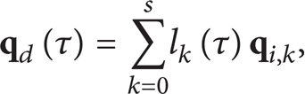
The Hamilton Principle of a multibody system with holonomic constraints and conservative forces can be stated as

$\delta S=\delta {\int }_{\mathrm{0}}^{t_f}\left(L(\mathbf{q},\dot{\mathbf{q}},t)-{\mathbf{\lambda }}^T\mathbf{\Phi }(\mathbf{q},t)\right)dt=\mathrm{0},$

(1)

where S is Hamilton action integral, L is Lagrangian, q, $\dot{\mathbf{q}}$ are generalized displacement and velocity, respectively, and λ is Lagrange multiplier vector corresponding to the constraint

$\mathbf{\Phi }\left(\mathbf{q},t\right)=\mathbf{0}\mathbf{.}$

(2)

Via variational method, the following Euler-Lagrange equations of a constrained mechanical system can be got:

$\begin{array}{c}\frac{d}{dt}\left(\frac{\partial L\left(\mathbf{q},\dot{\mathbf{q}},t\right)}{\partial \dot{\mathbf{q}}}\right)-\frac{\partial L\left(\mathbf{q},\dot{\mathbf{q}},t\right)}{\partial \mathbf{q}}+{\mathbf{\Phi }}^T\left(\mathbf{q},t\right)\mathbf{\lambda }=\mathbf{0}\mathbf{,}\\ \mathbf{\Phi }\left(\mathbf{q},t\right)=\mathbf{0}\mathbf{.}\end{array}$

(3)

It is a typical differential-algebraic equation which can be solved using different traditional numerical methods of DAEs [2, 3].

Following the variational integrators based on discrete variational principle, the time interval t∈[0,t _f ] is divided into N subintervals with time step h = t _f /N equally along with N + 1 grids, 0 = t₀,t₁,t₂,…, t_N–1, t _N = t _f , t _i = ih, i = 0,1,2,…, N. The discrete generalized displacement and velocity and Lagrangian multiplier can be denoted as q _i = q(t _i ), ${\dot{\mathbf{q}}}_i=\dot{\mathbf{q}}(t_i)$ , λ _i = λ(t _i ), i = 0,1,2,…, N. Equation (1) can be rewritten as the following discrete counterpart:

$\begin{array}{c}\delta S_d\left({\mathbf{q}}_{\mathrm{0}},{\mathbf{q}}_{\mathrm{1}},\dots ,{\mathbf{q}}_{N-\mathrm{1}},{\mathbf{q}}_N,{\mathbf{\lambda }}_{\mathrm{0}},\dots ,{\mathbf{\lambda }}_{N-\mathrm{2}},{\mathbf{\lambda }}_{N-\mathrm{1}}\right)\\ =\delta \sum _{i=\mathrm{0}}^{N-\mathrm{1}}{L}_d\left({\mathbf{q}}_i,{\mathbf{q}}_{i+\mathrm{1}},t_i\right)-\delta \sum _{i=\mathrm{0}}^{N-\mathrm{1}}{f}_d\left({\mathbf{q}}_i,{\mathbf{q}}_{i+\mathrm{1}},{\mathbf{\lambda }}_i,t_i\right)\\ =\mathrm{0},\end{array}$

(4)

where L _d (q _i ,q_{i + 1},h) and f _d (q _i ,q_{i + 1},λ _i ,t _i ) are defined as the discrete approximation of the integration of $L(\mathbf{q},\dot{\mathbf{q}},t)$ and λ ^T Φ(q,t) on the interval t∈[t _i ,t_{i + 1}],

$\begin{array}{c}{L}_d\left({\mathbf{q}}_i,{\mathbf{q}}_{i+\mathrm{1}},t_i\right)={\int }_{t_i}^{t_{i+\mathrm{1}}}L\left(\mathbf{q},\dot{\mathbf{q}},t\right)dt,\\ f_d\left({\mathbf{q}}_i,{\mathbf{q}}_{i+\mathrm{1}},{\mathbf{\lambda }}_i,t_i\right)={\int }_{t_i}^{t_{i+\mathrm{1}}}{\mathbf{\lambda }}^T\mathbf{\Phi }\left(\mathbf{q},t\right)dt.\end{array}$

(5)

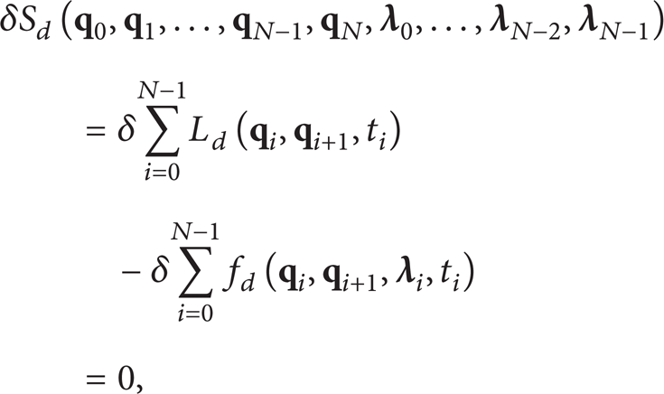
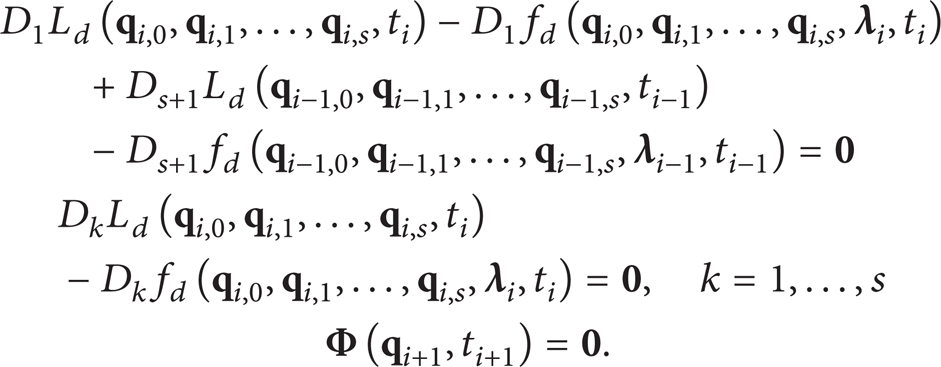
Using standard variational method, the discrete Euler-Lagrangian (DEL) equations are derived as

$\begin{array}{c}{D}_{\mathrm{1}}{L}_d\left({\mathbf{q}}_i,{\mathbf{q}}_{i+\mathrm{1}},t_i\right)+D_{\mathrm{2}}{L}_d\left({\mathbf{q}}_{i-\mathrm{1}},{\mathbf{q}}_i,t_{i-\mathrm{1}}\right)-h{\mathbf{\Phi }}_{\mathbf{q}}^T\left({\mathbf{q}}_i,t_i\right){\mathbf{\lambda }}_i=\mathbf{0}\mathbf{,}\\ \mathbf{\Phi }\left({\mathbf{q}}_{i+\mathrm{1}},t_{i+\mathrm{1}}\right)=\mathbf{0},\end{array}$

(6)

where D _j L _d (j = 1, 2) is the partial derivative of L _d with respect to the jth variable.

3. Higher Order Variational Galerkin Integrators of Multibody Systems with Constraints

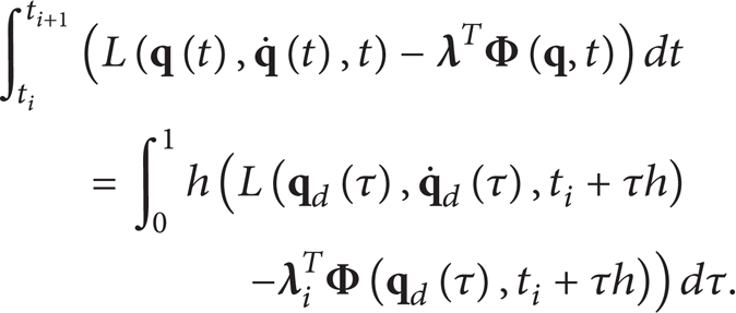
The key technique to improve the accuracy of variational integrators is the approximation of the discrete Hamiltonian action integral, which can be realized through general Galerkin methods [24, 25]. Using the same methods in this section, Hamiltonian action integral is approximated in a subinterval $[t_i,t_{i+\mathrm{1}}]$ with an introduced local time parameter $\tau \in [\mathrm{0,1}]$ , where

$\tau =\frac{t-t_i}{t_{i+\mathrm{1}}-t_i}.$

(7)

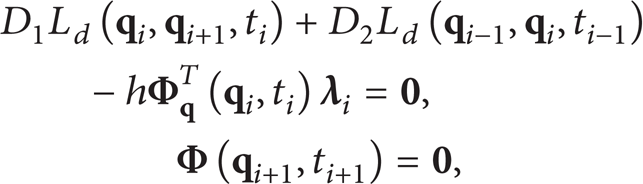
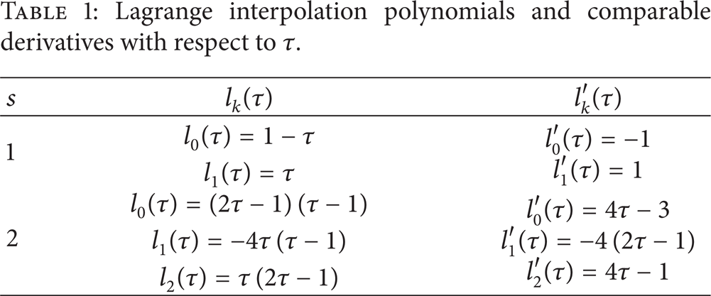
Given s + 1 control points 0 = τ₀<τ₁<⋯<τ _s = 1, for k = 0, 1,…, s, Lagrange interpolation polynomial l _k (τ):[0, 1]→R is defined as

$l_k\left(\tau \right)=\prod _{\mathrm{0}\le j\le s,j\ne k}\frac{\tau -{\tau }_j}{{\tau }_k-{\tau }_j}.$

(8)

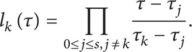
The state variables q(t) on $[t_i,t_{i+\mathrm{1}}]$ can be interpolated as follows:

${\mathbf{q}}_d\left(\tau \right)=\sum _{k=\mathrm{0}}^s{l}_k\left(\tau \right){\mathbf{q}}_{i,k},$

(9)

where ${\mathbf{q}}_{i,k}=\mathbf{q}(t_i+k·(h/s))$ . The derivative of q _d (τ) with respect to t provides an approximation of $\dot{\mathbf{q}}(t)$ on $[t_i,t_{i+\mathrm{1}}]$ as

${\dot{\mathbf{q}}}_d\left(\tau \right)=\frac{\mathrm{1}}{h}\sum _{k=\mathrm{0}}^s{l}_k^{\prime }\left(\tau \right){\mathbf{q}}_{i,k},$

(10)

where $l_k^{\prime }(\tau )=(\partial /\partial \tau )l_k(\tau )$ . Then, Hamiltonian action integral can be approximated on $[t_i,t_{i+\mathrm{1}}]$ as follows:

$\begin{array}{l}{\int }_{t_i}^{t_{i+\mathrm{1}}}\left(L(\mathbf{q}\left(t\right),\dot{\mathbf{q}}\left(t\right),t)-{\mathbf{\lambda }}^T\mathbf{\Phi }(\mathbf{q},t)\right)dt\\ ={\int }_0^{1}h(\phantom{{\mathbf{\lambda }}_i^T\mathbf{\Phi }({\mathbf{q}}_d\left(\tau \right),t_i+\tau h)}L({\mathbf{q}}_d\left(\tau \right),{\dot{\mathbf{q}}}_d\left(\tau \right),t_i+\tau h)-{\mathbf{\lambda }}_i^T\mathbf{\Phi }\left({\mathbf{q}}_d\left(\tau \right),t_i+\tau h\right))d\tau .\end{array}$

(11)

Lagrange interpolation polynomials in (9) and comparable derivatives with respect to τ in (10) are listed in Table 1.

Table 1:

Lagrange interpolation polynomials and comparable derivatives with respect to τ.

s	l k (τ)	l k ′(τ)
1	$\begin{array}{c}{l}_{\mathrm{0}}(\tau )=\mathrm{1}-\tau \\ l_{\mathrm{1}}(\tau )=\tau \end{array}$	$\begin{array}{c}{l}_{\mathrm{0}}^{\prime }(\tau )=-\mathrm{1}\\ l_{\mathrm{1}}^{\prime }(\tau )=\mathrm{1}\end{array}$
2	$\begin{array}{c}{l}_{\mathrm{0}}(\tau )=\left(\mathrm{2}\tau -\mathrm{1}\right)\left(\tau -\mathrm{1}\right)\\ l_{\mathrm{1}}(\tau )=-\mathrm{4}\tau \left(\tau -\mathrm{1}\right)\\ l_{\mathrm{2}}(\tau )=\tau \left(\mathrm{2}\tau -\mathrm{1}\right)\end{array}$	$\begin{array}{c}{l}_{\mathrm{0}}^{\prime }(\tau )=\mathrm{4}\tau -\mathrm{3}\\ l_{\mathrm{1}}^{\prime }(\tau )=-\mathrm{4}\left(\mathrm{2}\tau -\mathrm{1}\right)\\ l_{\mathrm{2}}^{\prime }(\tau )=\mathrm{4}\tau -\mathrm{1}\end{array}$

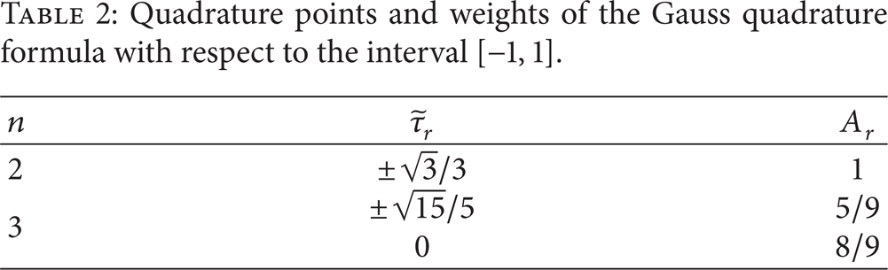
Using Gauss quadrature formula, which has maximal degree of accuracy 2n–1 for a fixed number n of quadrature points, we have

$\begin{array}{l}{\int }_{t_i}^{t_{i+\mathrm{1}}}\left(L(\mathbf{q}\left(t\right),\dot{\mathbf{q}}\left(t\right),t)-{\mathbf{\lambda }}^T\mathbf{\Phi }(\mathbf{q},t)\right)dt\\ =\sum _{r=\mathrm{1}}^n{A}_{r}h(\phantom{{\mathbf{\lambda }}_i^T\mathbf{\Phi }({\mathbf{q}}_d\left({\tilde{\tau }}_r\right),t_i+{\tilde{\tau }}_{r}h)}L\left({\mathbf{q}}_d\left({\tilde{\tau }}_r\right),{\dot{\mathbf{q}}}_d\left({\tilde{\tau }}_r\right),t_i+{\tilde{\tau }}_{r}h\right)-{\mathbf{\lambda }}_i^T\mathbf{\Phi }({\mathbf{q}}_d\left({\tilde{\tau }}_r\right),t_i+{\tilde{\tau }}_{r}h))\\ =L_d({\mathbf{q}}_{i,\mathrm{0}},{\mathbf{q}}_{i,\mathrm{1}},\dots ,{\mathbf{q}}_{i,s},t_i)-f_d\left({\mathbf{q}}_{i,\mathrm{0}},{\mathbf{q}}_{i,\mathrm{1}},\dots ,{\mathbf{q}}_{i,s},{\mathbf{\lambda }}_i,t_i\right),\end{array}$

(12)

where A _r is the weights and ${\tilde{\tau }}_r$ is the quadrature point. Quadrature points and weights of the Gauss quadrature formula with respect to the interval $[-1,1]$ are listed in Table 2.

Table 2:

Quadrature points and weights of the Gauss quadrature formula with respect to the interval [−1, 1].

n	${\tilde{\tau }}_r$	A r
2	$\pm \sqrt{\mathrm{3}}/\mathrm{3}$	1
3	$\pm \sqrt{\mathrm{15}}/\mathrm{5}$	5/9
	0	8/9

Apply discrete Hamilton's principle, the derivatives of the action with respect to q_i,k have to vanish for all i = 0, 1,…, N–1 and k = 0, 1,…, s. That leads to the discrete Euler-Lagrange equations

$\begin{array}{c}{D}_{\mathrm{1}}{L}_d\left({\mathbf{q}}_{i,\mathrm{0}},{\mathbf{q}}_{i,\mathrm{1}},\dots ,{\mathbf{q}}_{i,s},t_i\right)-D_{\mathrm{1}}{f}_d\left({\mathbf{q}}_{i,\mathrm{0}},{\mathbf{q}}_{i,\mathrm{1}},\dots ,{\mathbf{q}}_{i,s},{\mathbf{\lambda }}_i,t_i\right)+D_{s+\mathrm{1}}{L}_d\left({\mathbf{q}}_{i-\mathrm{1,0}},{\mathbf{q}}_{i-\mathrm{1,1}},\dots ,{\mathbf{q}}_{i-\mathrm{1},s},t_{i-\mathrm{1}}\right)-D_{s+\mathrm{1}}{f}_d\left({\mathbf{q}}_{i-\mathrm{1,0}},{\mathbf{q}}_{i-\mathrm{1,1}},\dots ,{\mathbf{q}}_{i-\mathrm{1},s},{\mathbf{\lambda }}_{i-\mathrm{1}},t_{i-\mathrm{1}}\right)=\mathbf{0}\\ D_k{L}_d\left({\mathbf{q}}_{i,\mathrm{0}},{\mathbf{q}}_{i,\mathrm{1}},\dots ,{\mathbf{q}}_{i,s},t_i\right)-D_k{f}_d\left({\mathbf{q}}_{i,\mathrm{0}},{\mathbf{q}}_{i,\mathrm{1}},\dots ,{\mathbf{q}}_{i,s},{\mathbf{\lambda }}_i,t_i\right)=\mathbf{0},\hspace{1em}k=\mathrm{1},\dots ,s\\ \mathbf{\Phi }\left({\mathbf{q}}_{i+\mathrm{1}},t_{i+\mathrm{1}}\right)=\mathbf{0}\mathbf{.}\end{array}$

(13)

4. Computation Procedure

The following computation procedure can be used to get the solution of the discrete Euler-Lagrange equations (13).

Step 1. Given the order of Lagrange interpolation polynomial s, the number of Gauss quadrature points n, fixed time step h, initial state variables q₀, and velocity variables ${\dot{\mathbf{q}}}_{\mathrm{0}}$ .

Step 2. Get q₁, ${\dot{\mathbf{q}}}_{\mathrm{1}}$ , and λ₁ by Euler method or Runge-Kutta method. Use q_0,0 = q₀, and q_0,s = q₁ to calculate q_0,k, k = 1,…, s–1.

Step 3. For i = 2 to N–1, solve (13) by Newton iteration method to get q_i,1,…,q_i,s and λi, thus q_{i + 1} = q_i,s, ${\dot{\mathbf{q}}}_{i+\mathrm{1}}={\dot{\mathbf{q}}}_d(\mathrm{1})=(\mathrm{1}/h){\sum }_{k=\mathrm{0}}^s{l}_k^{\prime }(\mathrm{1}){\mathbf{q}}_{i,k}$ .

Step 4. Use the solution qi, ${\dot{\mathbf{q}}}_{i+\mathrm{1}}$ , i = 0,1,…, N–1 to get the potential energy T, kinetic energy V, total energy of the system H = T + V, and constraints Φ.

5. Numerical Example

Consider a simple double pendulum system shown in Figure 1 the state variables are chosen as q = [x₁ y₁ x₂ y₂] ^T , then the potential energy, kinetic energy of the system are

$\begin{array}{c}T=\frac{\mathrm{1}}{\mathrm{2}}{m}_{\mathrm{1}}\left({\dot{x}}_{\mathrm{1}}^{\mathrm{2}}+{\dot{y}}_{\mathrm{1}}^{\mathrm{2}}\right)+\frac{\mathrm{1}}{\mathrm{2}}{m}_{\mathrm{2}}\left({\dot{x}}_{\mathrm{2}}^{\mathrm{2}}+{\dot{y}}_{\mathrm{2}}^{\mathrm{2}}\right),\mathrm{\hspace{0.17em}\hspace{0.17em}}\mathrm{\hspace{0.17em}\hspace{0.17em}}\mathrm{\hspace{0.17em}\hspace{0.17em}}\mathrm{\hspace{0.17em}\hspace{0.17em}}\mathrm{\hspace{0.17em}\hspace{0.17em}}\mathrm{\hspace{0.17em}\hspace{0.17em}}\mathrm{\hspace{0.17em}\hspace{0.17em}}\mathrm{\hspace{0.17em}\hspace{0.17em}}\mathrm{\hspace{0.17em}\hspace{0.17em}}\mathrm{\hspace{0.17em}\hspace{0.17em}}\mathrm{\hspace{0.17em}\hspace{0.17em}}\\ V=m_{\mathrm{1}}g{y}_{\mathrm{1}}+m_{\mathrm{2}}g{y}_{\mathrm{2}}.\end{array}$

(14)

The mass matrix is a constant matrix as follows:

$\mathbf{M}=\mathrm{diag}\left[\begin{array}{cccc}{m}_{\mathrm{1}}& m_{\mathrm{1}}& m_{\mathrm{2}}& m_{\mathrm{2}}\end{array}\right].$

(15)

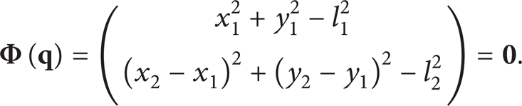
The constraint equations are

$\mathbf{\Phi }\left(\mathbf{q}\right)=\left(\begin{array}{c}{x}_{\mathrm{1}}^{\mathrm{2}}+y_{\mathrm{1}}^{\mathrm{2}}-l_{\mathrm{1}}^{\mathrm{2}}\\ {\left(x_{\mathrm{2}}-x_{\mathrm{1}}\right)}^{\mathrm{2}}+{\left(y_{\mathrm{2}}-y_{\mathrm{1}}\right)}^{\mathrm{2}}-l_{\mathrm{2}}^{\mathrm{2}}\end{array}\right)=\mathbf{0}\mathbf{.}$

(16)

Figure 1:

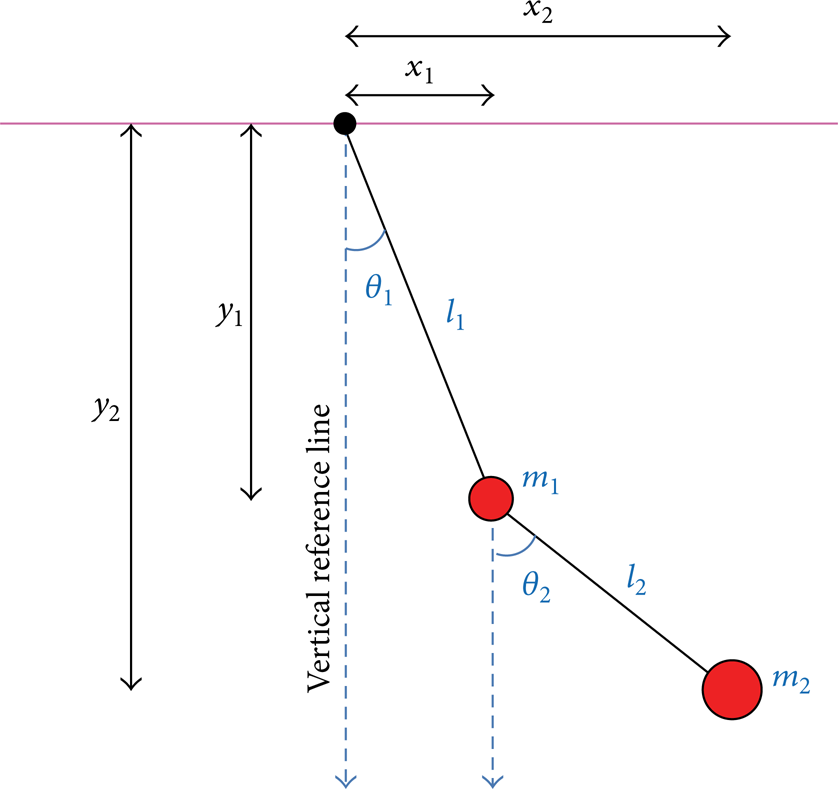
Double pendulum.

Given m₁ = m₂ = 1 kg, l₁ = l₂ = 1 m, with time step h = 0.01's, the results of the method presented in this paper are compared with the Runge-Kutta method in Table 3 for the terminal time 100's. Here, P1L-Q2G means that the order of Lagrange interpolation polynomial is 1 and the number of Gauss quadrature points is 2, and the same as P2L-Q2G and P2L-Q3G. ε(Η), ε(Φ) are the maximum errors of the total energy H and constraints Φ.

Table 3:

Comparison of the methods mentioned with time step h = 0.01.

Numerical method	Run time (s)	$\underset{}{\max }\left|\epsilon (H)\right|$	$\underset{}{\max }\left|\epsilon (\mathbf{\Phi })\right|$
Runge-Kutta	15.0385	3.0045	0.2345
P1L-Q2G	16.0993	0.4049	1.9984 × 10−15
P2L-Q2G	24.8510	0.2270	8.8818 × 10−16
P2L-Q3G	31.2938	0.2273	1.3323 × 10−15

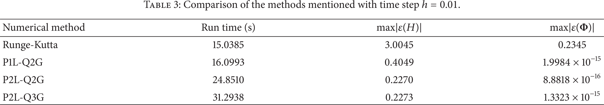
Using the traditional method such as Runge-Kutta method, to keep the errors of the total energy H and constraints Φ are all smaller, the time step should be chosen as about 0.001's in this example, and the total computation time is 99.7938's. But using the discrete variational methods presented in this paper, the time step can be chosen longer as 0.01's. Table 3 shows that, with this longer time step, the discrete variational methods can keep the total energy and constraints in higher accuracy than Runge-Kutta method, the cost instead is the longer computation time because of the iterations during the nonlinear equations solving process, but it is still shorter than the computation time of Runge-Kutta method with smaller time step to reach the same accuracy of the results.

It is also shown in Tables 3 and 4 that when the order of Lagrange interpolation polynomial is higher, the total energy and constraints can be kept better, but there are no big differences between 2 or 3 points in Gauss quadrature formula.

Table 4:

Comparison of the methods mentioned with time step h = 0.001.

Numerical method	Run time (s)	$\underset{}{\max }\left|\epsilon (H)\right|$	$\underset{}{\max }\left|\epsilon (\mathbf{\Phi })\right|$
Runge-Kutta	99.7938	4.7378 × 10−4	3.6633 × 10−5
P1L-Q2G	121.4468	0.0405	9.6040 × 10−11
P2L-Q2G	212.9882	0.0023	1.2912 × 10−9
P2L-Q3G	265.9505	0.0021	1.2912 × 10−9

Figure 2 shows the energies of the previously mentioned methods. With the time step h = 0.01's, the total energy is up and down around zero with little errors during the long-time simulation by the methods presented in this paper, while increases quickly during the simulation by Runge-Kutta method. The results of high order variational Galerkin integrators are better than low order integrators.

Figure 2:

Total energy of double pendulum by different method, h = 0.01.

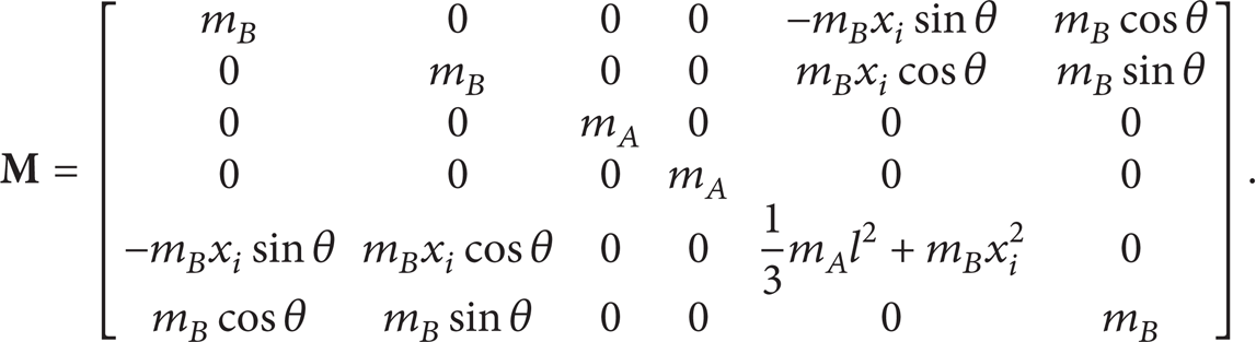
In the case of nonconstant mass matrix, the methods of higher order variational Galerkin integrators are also applicable. For another example, Figure 3 shows a rotary rod slider system. OA is a rigid rod with uniform mass m _A and length l, which rotates round O in the plane OXY. B is a slider with the mass m _B , and the stiffness of the spring on it is k; the mass of the spring is ignored. Suppose only gravity in the plane OXY is considered for the system.

Figure 3:

A rotary rod slider system.

The state variables are chosen as q = [R _{x ⁱ}  R _{y ⁱ}  R _{x ^j}  R _{y ^j} θ  x _i ] ^T . Then, the mass matrix is a nonconstant matrix

$\mathbf{M}=\left[\begin{array}{cccccc}{m}_B& \mathrm{0}& \mathrm{0}& \mathrm{0}& -m_B{x}_i\sin \theta & m_B\cos \theta \\ \mathrm{0}& m_B& \mathrm{0}& \mathrm{0}& m_B{x}_i\cos \theta & m_B\sin \theta \\ \mathrm{0}& \mathrm{0}& m_A& \mathrm{0}& \mathrm{0}& \mathrm{0}\\ \mathrm{0}& \mathrm{0}& \mathrm{0}& m_A& \mathrm{0}& \mathrm{0}\\ -m_B{x}_i\sin \theta & m_B{x}_i\cos \theta & \mathrm{0}& \mathrm{0}& \frac{\mathrm{1}}{\mathrm{3}}{m}_A{l}^{\mathrm{2}}+m_B{x}_i^2& \mathrm{0}\\ m_B\cos \theta & m_B\sin \theta & \mathrm{0}& \mathrm{0}& \mathrm{0}& m_B\end{array}\right].$

(17)

The constraint equations are

$\mathbf{\Phi }=\left(\begin{array}{c}{R}_{x^j}-\frac{l}{\mathrm{2}}\cos \theta \\ R_{y^j}-\frac{l}{\mathrm{2}}\sin \theta \\ \left(R_{x^j}-R_{x^i}\right)\cos \theta +\left(R_{y^j}-R_{y^i}\right)\sin \theta -x_i\\ \left(R_{x^j}-R_{x^i}\right)\sin \theta -\left(R_{y^j}-R_{y^i}\right)\cos \theta \end{array}\right)=\mathbf{0}\mathbf{.}$

(18)

Given l₁ = 2m, m _A = 2 kg, m _B = 5 kg, k = 1000 N/m. With the initial step length h = 0.01's and the terminal time 100's, using the method P1L-Q2G, where the order of Lagrange interpolation polynomial is 1 and the number of Gauss quadrature points is 2, the results are also satisfying. The total computer time is 86.0034's; the maximum errors of the total energy H and constraints Φ are 0.2611 and 3.8858 × 10⁻¹⁶, which is illustrated in Figures 4 and 5.

Figure 4:

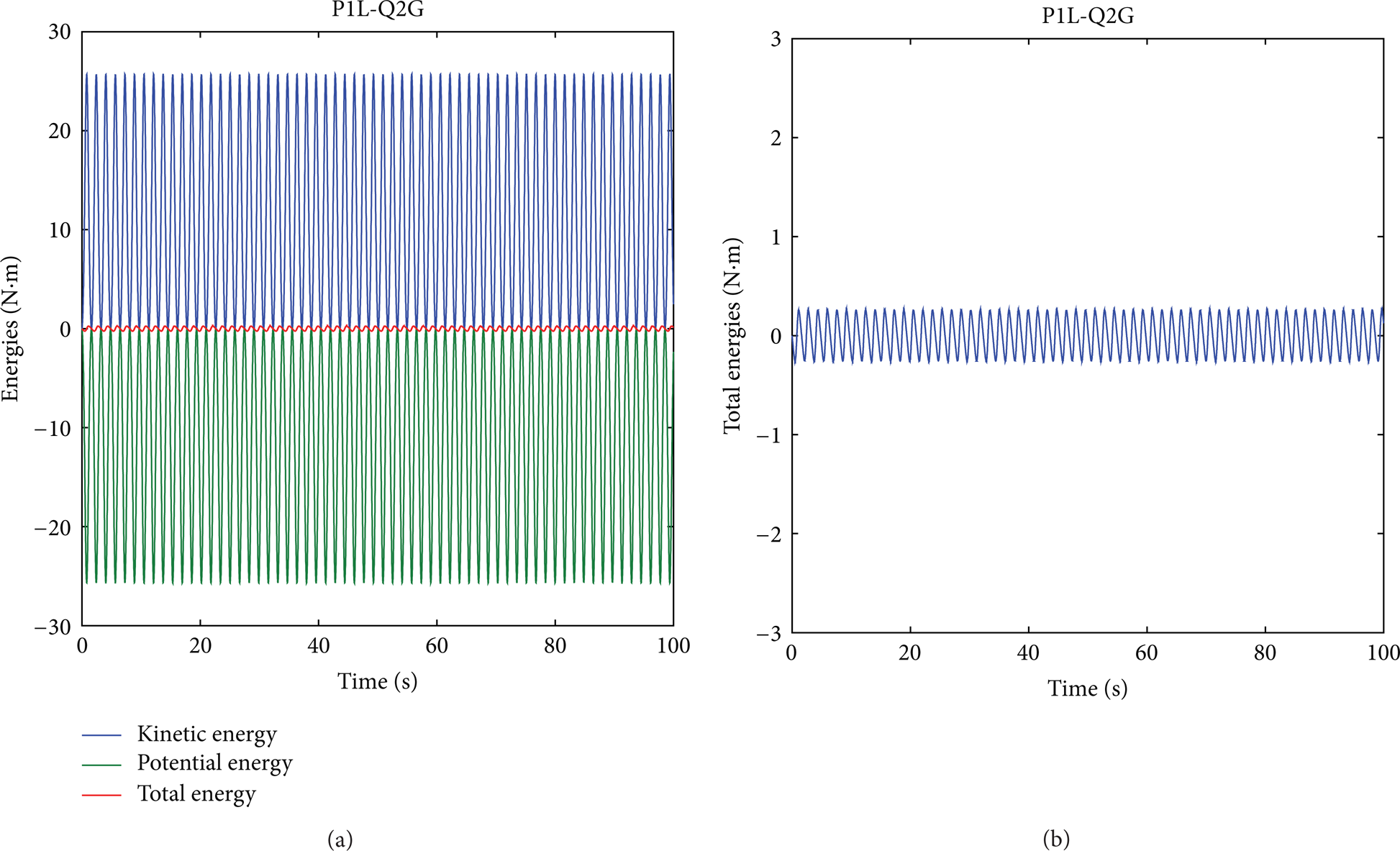
Energies of rotary rod slider system by method P1L-Q2G, h = 0.01.

Figure 5:

Constraints of rotary rod slider system by method P1L-Q2G, h = 0.01.

6. Conclusions

Based on Lagrange interpolation and Gauss quadrature, higher order variational Galerkin integrators have been developed for multibody systems with constraints. Numerical results validate the accuracy of the method for longer time step and long-time simulation. Nevertheless, as the computation is more complex, the computation cost is higher. Further study is needed to have more efficient integrators.

Conflict of Interests

The authors declare that there is no conflict of interests regarding the publication of this paper.