Broadcast Aggregation to Improve Quality of Service in Wireless Sensor Networks

Abstract

In-network aggregation is used in wireless sensor networks to reduce energy consumption on sensor nodes with limited capabilities. Typically, only packets with the same destination are aggregated along the routing path and these packets are sent by unicast. While this is adequate for traditional multipoint-to-point sensor network applications, this is not suitable when wireless sensor nodes are connected in a full mesh topology, as isthe case in the Internet of Things. In these full mesh topologies, queues will be filled with packets with many different destinations, which limits the aggregation possibilities. Furthermore, the Quality of Service level will decrease since packets have to wait longer to find aggregation candidates. Therefore, in this paper, we propose to use broadcast aggregation that can aggregate packets independent of their destination. Broadcast aggregation is analyzed through simulations against unicast aggregation and no aggregation. Results show that energy can be reduced up to 13% compared with unicast aggregation and up to 27% compared with no aggregation. In terms of reliability, the Quality of Service is improved up to 15% compared with unicast aggregation and up to 23% compared with no aggregation. The delay on its turnis decreased by 52% compared with unicast aggregation.

1. Introduction

Reducing energy consumption in wireless sensor networks has been extensively studied in recent years. Wireless sensor networks are networks that contain low-power and low-cost sensor nodes that are communicating through a wireless radio interface. These sensor nodes are often battery powered, and hence energy is a scarce resource [1]. A technique that is often used to reduce energy consumption is in-network aggregation [2]. In traditional in-network aggregation, many packets with the same (next-hop) destination are aggregated into one big packet and the aggregated packet is sent along the routing path by unicast messages. As a consequence, fewer transmissions and receptions are needed, and since radio communication consumes most of the sensor network energy, energy is saved by reducing the radio-on time.

However, the impact of in-network aggregation on the Quality of Service (QoS) level is currently not fully addressed and the trade-off between energy and QoS is often ignored. In previous work [3], we have already studied the impact of in-network aggregation on energy, delay, and reliability and we presented a tunable QoS-aware in-network aggregation scheme that makes a trade-off between energy consumption and a predefined QoS level. But we have observed that this technique works only well when there are many aggregation opportunities, which is true for traditional source-to-sink applications.

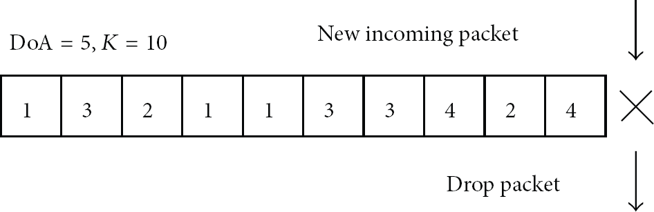
Today, more and more sensor networks are interconnected with the Internet, forming what is called the Internet of Things (IoT). For example, Libelium [4] lists 57 sensor applications for a smarter world situated in home, environments, industry, healthcare, and many more. These sensor nodes will join the Internet dynamically and use it to collaborate and accomplish their task [5]. A drawback is that there are many different communication paths which can lead to fewer aggregation opportunities and fewer packets that can be aggregated into one single packet (in the following referred to as the degree of aggregation, DoA) since the queues on the nodes become filled with packets with many different destinations. As a consequence, more energy is wasted and the QoS level is decreased since packets will have to wait longer resulting in a higher drop probability.

Therefore, in this paper, we propose to use broadcast aggregation to aggregate packets independent of their next-hop destination. We show that applying broadcast aggregation leads to faster aggregation with a higher overall QoS level and lower energy consumption.

The remainder of this paper is organized as follows. Section 2 gives an overview of the related work on QoS-aware unicast and broadcast in-network aggregation, while in Section 3 the applied broadcast mechanism is explained. A definition and problem statement is given first, followed by a performance analysis. Simulation results are discussed in Section 4. We end this paper with a conclusion and a look on future work in Section 5.

2. Related Work

Because energy is a main concern in wireless sensor networks and in-network aggregation is very suited to reduce energy consumption, in-network aggregation has been already extensively studied in recent years [2, 6]. Since packets are often exchanged by unicast messages or by broadcast messages, in-network aggregation protocols can be classified into unicast-based in-network aggregation protocols and broadcast-based in-network aggregation protocols. As we focus on both energy consumption and QoS, we limit ourselves to lossless QoS-aware in-network aggregation approaches. With lossless we mean that the initial data can be reconstructed and we do not consider aggregation functions such as minimum, maximum, and average.

In unicast-based in-network aggregation, aggregation is performed along the intermediate nodes of the routing path. It goes without saying that the routing algorithm and the routing path have a profound influence on the performance of the in-network aggregation. Examples can be found in [7–10].

In LUMP [7], a simple data aggregation protocol which enables QoS support for applications is proposed. Therefore, it prioritizes packets for differentiated services and facilitates aggregation decisions. The architecture has a cross-layer design and is a completely independent module residing between data link and network layer. The priority level represents the tolerable end-to-end latency of the packet.

The authors of [8] investigate data gathering and aggregation in a distributed, multihop sensor network under specific QoS constraints. Firstly, delay controlled Data Aggregation and Processing (Q-DAP) is performed at the intermediate nodes in a distributed fashion. Each node can decide independently if it performs aggregation. If the delay constraint can be satisfied, the report is deferred for a fixed time interval with a certain probability; otherwise, it is sent to the next hop. If it cannot be satisfied in any case, it is discarded. Secondly, a Localized Adaptive Data Collection and Aggregation (LADCA) approach is proposed for the end nodes. This algorithm defines the data sample rate taking into account energy-efficiency, delay, accuracy, and buffer overflow.

In [9], Padmanabh and Vuppala present an adaptive data aggregation algorithm with bursty sources in wireless sensor networks. In this paper, both lossy and lossless aggregation schemes are taken into account. Furthermore, the degree of aggregation is a controllable parameter and buffer management is used to optimize the QoS by minimizing the packet loss due to buffer overflow.

Finally, Akkaya et al. [10] describe an algorithm for achieving maximal possible energy savings through data aggregation while meeting the desired level of timeliness. In order to perform service differentiation and ensure bounded delay for constrained traffic, a weighted fair queuing based mechanism is employed.

Broadcast-based in-network aggregation takes advantage of the density of sensor networks in which one sensor node often has many neighbors. By broadcasting a packet, the packet can be received by many neighboring nodes, and for this reason, this approach is often used to increase reliability of multipath routing.

Most broadcast-based in-network aggregation techniques in the literature focus however on lossy aggregation (by using aggregation functions such as minimum, maximum, and average) and sending this aggregated value by multiple paths to the sink. A focus hereby is developing duplicate-sensitive aggregation functions since broadcast aggregation can lead to incorrect values at the sink node [11–14]. This is however out of scope of this paper.

In AIDA [15], a lossless adaptive application-independent data aggregation mechanism is presented. This solution contains an aggregation module that resides between the data link and network layer. Aggregation decisions are made in accordance with an adaptive feedback-based packet-scheduling scheme that dynamically controls the degree of aggregation in accordance with the MAC delay. This dynamic feedback scheme is based on the overall queuing delay imposed on AIDA payloads that are waiting for transmission. The default degree of aggregation is 1, while if the traffic builds up, a greater degree of aggregation is allowed prior to sending. If the packets that are ready to be aggregated are targeting the same next-hop node, AIDA sends a manycast packet (or a unicast packet in the case that there is only one packet) with the target node specified. However, when there are network packets that have to be aggregated with a different next-hop address, these packets are aggregated into a single packet and the MAC broadcast address is used as destination. A drawback of AIDA is that it only tries to reduce end-to-end delay, and energy consumption is more considered as benefit than as trade-off value. Our focus is on energy reduction within the QoS constraints.

3. Broadcast Aggregation

3.1. Definition and Problem Statement

When performing in-network aggregation, there will always be a trade-off between energy and QoS. For instance, a higher degree of aggregation will lead to less energy consumption, but packets will have to wait longer in the queue and, as a consequence, the delay increases. Since in this paper the focus is both on energy reduction and QoS improvement, we try to send as much packets with the highest possible degree of aggregation, within the limits of the given QoS constraints. So packets will be kept in the queue as long as the maximum degree of aggregation (or the maximum number of packets that physically can be aggregated into one single packet) is not reached. However, since packets will have a limit on their maximum end-to-end delay, a timeout time is introduced. This is the time that a packet maximally may reside inside a node before it should be sent to the next-hop node.

The number of packets that can be aggregated into a single packet strongly depends on the protocols being used for transferring application data. Highly compact proprietary solutions can be used leading to a high DoA. However, even when using IETF-based IoT protocols (e.g., 6LoWPAN, UDP, and CoAP [16]) up to 5 packets can be aggregated as can be seen in Figure 1. Including the PHY header, the MAC header and footer, and the compressed 6LoWPAN/UDP header for link-local addresses, this leaves us up to 8 bytes for the application header and data, which should be sufficient for simple sensor network transactions such as temperature, humidity, or light responses. When using CoAP as the application protocol, a typical CoAP response without any options consumes 4 bytes for the CoAP header and 1 byte for the payload marker, leaving 3 bytes available for the actual payload.

Figure 1

Minimal aggregated packet structure for Internet of Things packets based on 802.15.4 packets with SYNC (synchronization) header, PHY (physical) header, MHR (MAC header), MFR (MAC footer), and compressed 6LoWPAN/UDP header for link-local addresses where up to 5 packets can be aggregated.

In traditional unicast aggregation, many small packets with the same (next-hop) destination are aggregated into one big packet and sent by unicast to the next-hop node along the routing path. In typical source-to-sink applications such as temperature monitoring, there are many aggregation possibilities since many packets are routed to the sink. A high degree of aggregation is possible and, as a consequence, much energy can be saved and QoS is only marginally affected.

However, in the IoT, a huge amount of devices may be interconnected with many bindings between individual devices (e.g., sensor-actuator interactions), and as a consequence, many different nodes can send packets to many different destination. Each intermediate routing node may contain many packets that have to be routed to different destinations. This leads to fewer aggregation candidates, so packets will have to be routed without being aggregated, or with a lower degree of aggregation. However, when both the timeout time and the predefined $\text{Do}{\text{A}}_{\max }$ value (= the maximum number of packets that can be aggregated into one single packet) are not yet reached, packets will be dropped because the queue is fully occupied with packets that are waiting for the required number of aggregate candidates or for their timeout time. This is illustrated in Figure 2. Alternatively, instead of dropping packets, we could also send packets before their timeout time, but this will again increase the energy consumption. Furthermore, more packets that are not aggregated will lead to more packets in the air and a higher drop probability due to channel issues (collisions, etc.).

Figure 2

Queue overflow with predefined $\text{Do}{\text{A}}_{\max }=\mathrm{5}$ and maximum queue size $K=\mathrm{10}$ . A packet drop occurs since a new packet enters the system while the queue is fully occupied with packets that are waiting for the required number of aggregate candidates or for their timeout time.

To overcome these issues, we propose to use broadcast aggregation. Instead of aggregating packets with the same (next-hop) destination and sending them by unicast, packets are aggregated independent of their (next-hop) destination and sent by broadcast. This decouples aggregation from the routing path. In unicast communication, packets are sent to a single destination on the routing path, while by broadcast communication, a transmitted packet is received by every node within the coverage area. The receiving nodes can then extract the packet and retrieve the packet parts that are destined for them. This broadcast aggregation mechanism is visualized in Figure 3.

Figure 3

Broadcast aggregation mechanism: nodes 1, 2, and 3 send data packets (resp., $\hspace{0.17em}\hspace{0.17em}X$ , Y, and Z) sequentially ( $t_{\mathrm{1}}<t_{\mathrm{2}}<t_{\mathrm{3}}$ ) towards, respectively, nodes 7, 6, and 5. These packets wait in the intermediate node (node 4) until the requested DoA is reached and then they are aggregated independent of their next-hop destination. This aggregated packet is then sent by broadcast on $t_{\mathrm{4}}$ to the neighboring nodes. Destination nodes 5, 6, and 7 can then extract the data part that is destined for them (resp., Z, Y, and X).

3.2. Performance Analysis

In the following, we compare broadcast aggregation with unicast aggregation. As already explained in Section 3.1, broadcast aggregation is performed as soon as the number of available packets reaches the predefined $\text{Do}{\text{A}}_{\max }$ value or when the maximum timeout time has reached.

To summarize, broadcast aggregation is performed.

• (i)

When there are $\text{Do}{\text{A}}_{\max }$ packets in the system, $\text{Do}{\text{A}}_{\max }$ packets are aggregated and sent by broadcast $\Rightarrow B=\text{Do}{\text{A}}_{\max }$

(ii)

When fewer than $\text{Do}{\text{A}}_{\max }$ packets are in the system and the maximum timeout time has reached for at least one of the packets $\Rightarrow B<\text{Do}{\text{A}}_{\max }$ .

With B the number of packets that are aggregated in a single packet that is broadcasted to all 1-hop neighbors.

For unicast aggregation, it is not possible to select the first $\text{Do}{\text{A}}_{\max }$ packets since these packets can have different next-hop destinations.

Unicast aggregation is therefore performed.

• (i)

When there are $\text{Do}{\text{A}}_{\max }$ packets with the same next-hop destination in the system $\Rightarrow U=\text{Do}{\text{A}}_{\max }$

(ii)

When fewer than $\text{Do}{\text{A}}_{\max }$ packets with the same next-hop destination are in the system and the maximum timeout time has reached for at least one of the packets with the same next-hop destination   $\Rightarrow U<\text{Do}{\text{A}}_{\max }$ .

With U the number of packets that are aggregated in a single packet that is sent to a single next-hop node using unicast.

To compare the broadcast aggregation with unicast aggregation, we can use the $M/M/\mathrm{1}/GD/K/\infty$ queuing system. This is a queuing system in which the interarrival times and service time are exponentially distributed with rate λ and rate μ, respectively. There is only one serving unit and there is a general queue discipline. However, only K packets can enter the system. This queuing system is shown in Figure 4.

Figure 4

$M/M/\mathrm{1}/GD/K/\infty$ queuing system.

For $\lambda \ne \mu$ and with $\rho =\lambda /\mu$ the steady-state probabilities are given by:

$$\begin{array}{l}{p}_{\mathrm{0}}=\frac{\mathrm{1}-\rho }{\mathrm{1}-{\rho }^{K+\mathrm{1}}},\\ p_i={\rho }^i{p}_{\mathrm{0}}\hspace{1em}\left(i=\mathrm{1,2},\dots ,K\right),\\ p_i=\mathrm{0}\hspace{1em}\left(i=K+\mathrm{1},K+\mathrm{2},\dots \right).\end{array}$$

(1)

3.2.1. Reliability

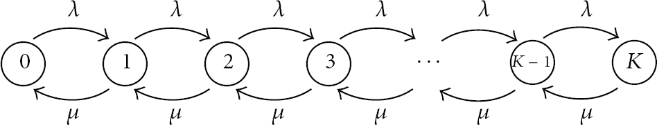
In a $M/M/\mathrm{1}/GD/K/\infty$ queuing system, the drop probability equals the probability that a new packet arrives when there are already K packets in the queue. Substituting $p_{\mathrm{0}}$ in $p_K$ , the reliability can be expressed as

$$\begin{array}{cc}& R=\mathrm{1}-p_K=\mathrm{1}-\frac{{\rho }^K\left(\mathrm{1}-\rho \right)}{\mathrm{1}-{\rho }^{K+\mathrm{1}}}.\end{array}$$

(2)

In Figure 5, the reliability (or the chance that a packet is not dropped from the queue) is shown for different μ values. The evaluation of (2) is done for $K=\mathrm{15}$ . This is a realistic assumption of the available buffer space on today's sensor nodes. For instance, the Zolertia Z1 sensor node [17] has 8 kB of RAM, but 4–6 kB is often used for code, which leaves only 2–4 kB for buffering. We can see from the figure that doubling the service rate can significantly improve the reliability, or in other words, doubling the service rate leads to an increased load capacity before a packet will be dropped.

Figure 5

Reliability analysis for different μ values (with μ the service rate, λ the interarrival rate, and $K=\mathrm{15}$ the maximum queue occupation).

So when broadcast aggregation is applied and the maximum timeout time has not passed, packets can be aggregated as soon as there are enough packets to meet the $\text{Do}{\text{A}}_{\max }$ value which will prevent from queue overflows. In unicast aggregation, the network topology determines the service rate since when there are many different streams with different next-hop destinations; it can take some time before there are enough packets with the same next-hop destination before aggregation can occur. So while B and U are the same, B will be reached earlier, which releases the queue earlier and increases the reliability.

In this section, we mentioned the node reliability caused by queue overflows. The end-to-end reliability will also be influenced by specific protocol implementations and channel related issues (e.g., collisions).

3.2.2. Delay

The delay or the average time that a packet resides in a node can be calculated from Little's queuing formula:

$$\begin{array}{cc}& D_{\text{avg}}=\frac{\overline{N}}{{\lambda }_{\text{eff}}}\end{array}$$

(3)

with $\overline{N}$ the average number of packets in the node and ${\lambda }_{\text{eff}}$ the average number of packets that actually enter the node. Recall that some packets may arrive in a fully occupied queue and will hence be dropped. These packets are not considered in ${\lambda }_{\text{eff}}$ .

${\lambda }_{\text{eff}}$ can be calculated as

$$\begin{array}{cc}& {\lambda }_{\text{eff}}=\sum _{k=\mathrm{0}}^K‍{\lambda }_k{p}_k=\lambda (\mathrm{1}-p_K)\end{array}$$

(4)

and $\overline{N}$ can be calculated as

$$\begin{array}{cc}& \overline{N}=\sum _{k=\mathrm{0}}^K‍k·p_k.\end{array}$$

(5)

Combining (3) with (4), (5), and (1), the average delay $D_{\text{avg}}$ that a packet resides inside the system can be expressed as follows:

$$\begin{array}{cc}& D_{\text{avg}}=\frac{\rho \left[\mathrm{1}-(K+\mathrm{1}){\rho }^K+K{\rho }^{K+\mathrm{1}}\right]}{\left(\mathrm{1}-{\rho }^{K+\mathrm{1}}\right)\left(\mathrm{1}-\rho \right)\lambda \left(\mathrm{1}-\left({\rho }^K\left(\mathrm{1}-\rho \right)/(\mathrm{1}-{\rho }^{K+\mathrm{1}})\right)\right)}.\end{array}$$

(6)

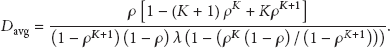
In Figure 6, the average delay is given for different μ values that are expressed in terms of the initial arrival rate λ. The evaluation of (6) is done for $K=\mathrm{15}$ . We can see from the figure that doubling the service rate can significantly reduce the average delay that a packet resides inside the system. So again, while B and U are the same, B will be reached earlier, which decreases the average (end-to-end) delay.

Figure 6

Delay analysis for different μ values (with μ the service rate, λ the interarrival rate, and $K=\mathrm{15}$ the maximum queue occupation).

3.2.3. Throughput

The end-to-end throughput of the network is expressed as the average rate of successfully delivered data from source to destination. This end-to-end throughput is influenced by two parts: a node throughput and a channel throughput. The node throughput equals the service rate μ. The channel throughput depends on channel overhead, transmission errors, and so forth. Aggregation in general is beneficial for channel utilization since fewer packets have to contend for the medium which leads to fewer packet drops.

3.2.4. Energy

In [3], we have shown that energy consumption can be reduced when aggregation is applied together with a sleep-wake-up scheme. Aggregation leads to fewer transmissions and receptions which results in more sleep opportunities and a reduced energy consumption level. The transmission energy consumption can be calculated as

$$\begin{array}{cc}& E_{\text{tx}}^{\text{reduction}}=\mathrm{1}-\frac{E_{\text{A}}}{E_{\text{NA}}}\end{array}$$

(7)

in which $E_{\text{A}}$ is the total transmission energy consumed when aggregation is performed and $E_{\text{NA}}$ is the total energy consumed when no aggregation is performed. Expressing $E_{\text{A}}$ in terms of $E_{\text{NA}}$ , this leads to

$$\begin{array}{cc}& E_{\text{tx}}^{\text{reduction}}\approx \mathrm{1}-\frac{E_{\text{TO}}+E_{\text{H}}^{\text{A}}+\text{Do}{\text{A}}_{\text{avg}}{E}_{\text{DATA}}^{\text{NA}}}{E_{\text{TO}}+E_{\text{H}}^{\text{NA}}+E_{\text{DATA}}^{\text{NA}}}\frac{\mathrm{1}}{\text{Do}{\text{A}}_{\text{avg}}}\end{array}$$

(8)

in which $E_{\text{TO}}$ is the energy consumption caused by transmission overhead per packet transmission. This contains the Clear Channel Assessment (CCA) time, the RX-TX turnaround time but also the overhead created by the MAC protocol, for example, by beacons. $E_{\text{H}}^{\text{NA}}$ is the energy consumed to send a not aggregated packet header, $E_{\text{H}}^{\text{A}}$ is the energy consumed to send a header of an aggregated packet, and $E_{\text{DATA}}^{\text{NA}}$ is the energy consumed to send individual data parts.

From (8), we can see that the energy reduction depends on the average DoA level ( $\text{Do}{\text{A}}_{\text{avg}}$ ). In general, the more packets that are aggregated (= a higher $\text{Do}{\text{A}}_{\text{avg}}$ ), the more energy that will be saved. Because in broadcast aggregation more packets are faster aggregated, more energy will be saved.

However, the total energy consumption will also depend on the applied sleep-wake-up scheme and the used MAC protocol. Since the impact is very protocol specific, this will be further discussed in the simulation results.

4. Simulation Results

4.1. Reliability

Simulations are done using Castalia, an OMNeT++ based network simulator for simulating wireless sensor networks [18]. We use a network scenario with 256 nodes, deployed in a square grid with size 75 m. This setup was chosen according to the RFC which describes the requirements for home automation routing in low power and lossy networks [19]. An own implementation of the DYMO protocol is chosen as routing protocol and the low power listening tunable MAC protocol that is available in the Castalia simulator is chosen as MAC protocol. The protocol operation is shown in Figure 7. Before node A transmits its data, it sends a CCA message to check if the channel is clear. If the medium is free, it starts periodically sending small beacon messages during a whole sleep interval. Afterwards, the actual data is sent. When node B receives a beacon message, it stays awake until the data transmission has finished. After this reception, it waits a listen interval before going back to sleep because other packets can follow. This behavior is the same for each node that receives beacon messages, regardless of the fact that this node is the destination for the actual data or not. Simulations are performed with $\text{DoA}=\mathrm{5}$ and with maximum queue size $K=\mathrm{15}$ .

Figure 7

Operation of the tunable MAC protocol. Node A sends a data packet to node B by first performing CCA, afterwards sending beacon messages, and finally sending the data packet. Node B stays awake when it receives one or more beacon messages until the data transfer is completed. Node C cannot receive these beacon messages and will again go to sleep after the listen interval.

In our scenario, each node (except the destination nodes) is transmitting packets to one of 20 randomly chosen destination nodes. A simulation lasts 3600 seconds, but statistics are generated in steady state between 300 and 3000 seconds. After 100 seconds, the network is up and running and the DYMO routes remain active during the entire simulation, as can be seen in Figure 8. This is, for instance, the case when there is a fixed communication between the sensor and actuator with regular traffic. The large amount of network setup traffic can be explained by the broadcast nature of the RREQ messages sent by the DYMO routing protocol. Simulation statistics later than 3000 seconds are not counted to ensure that all generated packets can reach their destination within the evaluated time. Furthermore, simulations are performed for different average traffic rates (from 1 to 30 packets/min) as given on the x-axis of the figures. For instance, when the average traffic rate is 5 packets/min, nodes choose a random traffic rate between 1 and 10 packets/min and send their packets according to this traffic rate without jitter. A higher average packet rate will lead to a higher network load. To assess the realism of these traffic rates, we can consider a scenario where a resource on a sensor node (e.g., the temperature) is being monitored using the CoAP observe option. In this case, the sensor node will send a notification every time the resource state changes (e.g., the temperature) or when its max-age value, which indicates the freshness of the resource state, expires. The default max-age value is 60 seconds, resulting in a minimum traffic rate of 1 packet/min. When values change more frequently, more messages will be sent. The maximum packet timeout was set to 10 seconds. This value gives nodes at low traffic rates enough time to find aggregate candidates before their timeout time passes. The used simulation settings can be found in Table 1.

Table 1

Simulation settings.

Parameter	Value
Simulation time	2700 s
Simulation field	75 m $\times$ 75 m
Number of nodes	256
Node deployment	$\mathrm{16}\times \mathrm{16}$ grid
Routing protocol	DYMO
MAC protocol	Tunable CSMA based MAC (Castalia)
	with duty cycle 0.2 (100 ms listening/400 ms sleeping)
Radio	CC2420 with no transmission errors
Wireless channel	No interference
Collision domain	$\pm$ 16 m, depends on the receiver signal strength
	( $\pm$ 2 hops)
Queue size (K)	15
DoA	5

Figure 8

Steady state calculation.

Figure 9 shows the overall reliability as the number of application packets received compared to the number of application packets sent. Figures 10 and 11 show, respectively, the number of packets dropped in the queue and the number of packets dropped due to the lower network layers (Radio, MAC, Physical channel). The packet error rate (PER) is expressed as the number of application packets dropped compared to the number of application packets sent. Packets in the queue are dropped due to queue overflows, while packets dropped by the lower layers are caused by the fact that a sensor node cannot simultaneously send and receive, and packets can collide.

Figure 9

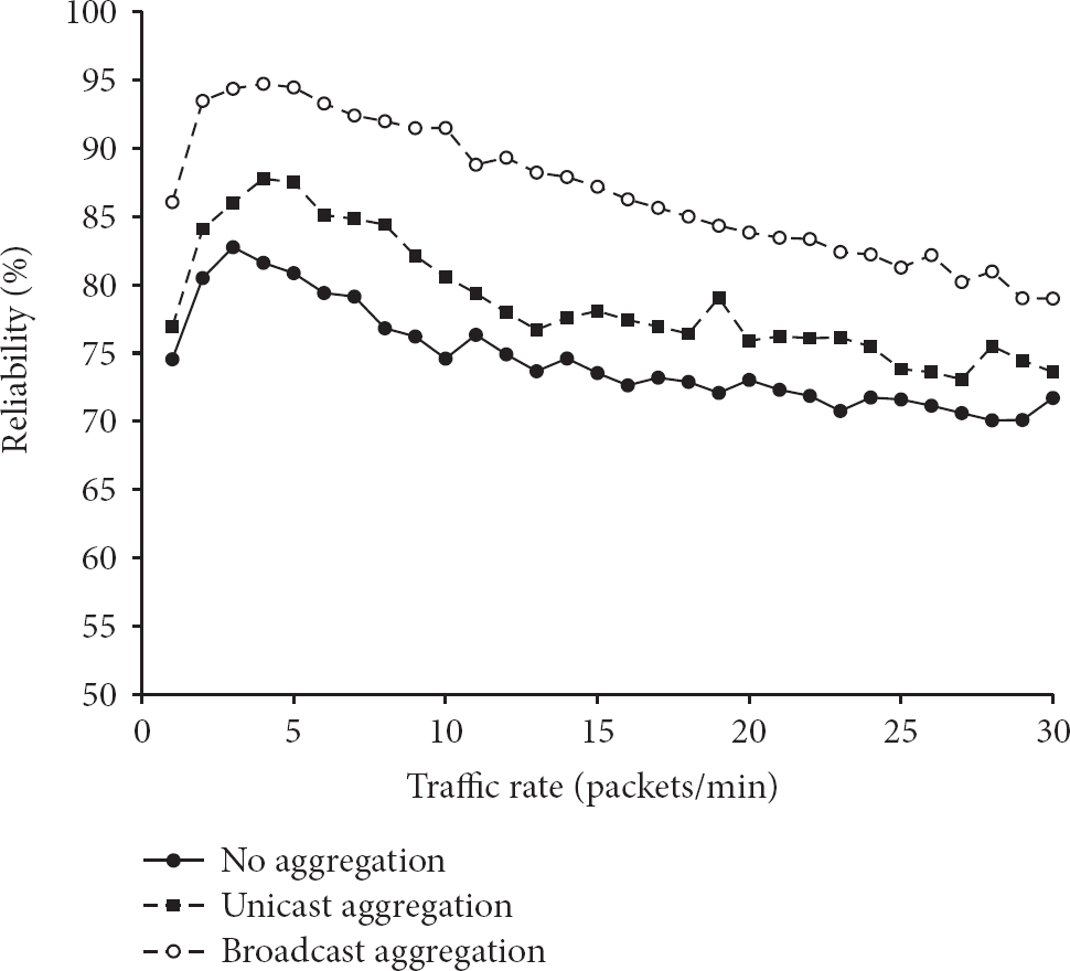
End-to-end reliability.

Figure 10

Packet error rate (PER): number of dropped packets in the queue compared with the number of packets sent.

Figure 11

Packet error rate (PER): number of dropped packets due to the lower network layers compared with the number of packets sent.

From Figure 10, we can see that for unicast aggregation, starting from an average traffic rate of 3 packets/min, packet drops occur in the queue. This is not the case in the no aggregation and broadcast aggregation scenario, since in the no aggregation scenario, packets do not have to wait for aggregation candidates and can be sent immediately. In the broadcast aggregation scenario, aggregated packets can be sent as soon as there are 5 packets in the queue. This effect can be seen in Figure 12 that shows the average queue occupation. We can see that the average queue occupation is on average 2 packets lower for broadcast aggregation than for unicast aggregation.

Figure 12

Average queue occupation.

Figure 11 shows on its turn the impact of the lower network layers on the reliability. The figure shows that in the beginning the packet error rate (PER) is relative high, then drops, and finally slowly increases again. The high PER at low traffic rates can be explained by the fact that each node will have approximately the same packet rate. Remember that the packet rate on the x-axis is the average packet rate of all the nodes. So at low packet rates, most sensor nodes will have the same packet rate and will try to enter the medium on the same time. As a consequence, more packets will be lost. From an average traffic rate of 5 packets/min, the PER starts increasing since more packets are in the air, which leads to a higher PER. Furthermore, we can see that the PER is higher in the no aggregation scenario, since when packets are not aggregated, more packets are in the air and more packets can be lost.

Since both unicast and broadcast aggregation combine packets into one big packet, we should expect that the packet loss due to the lower network layers should be approximately the same. This is however not the case at low traffic rates. This can be explained by a fact to which we refer in the following as “partial aggregation.”

A “partly aggregated” packet is a packet that contains fewer than DoA aggregated packet parts. For instance, when the DoA was set to 5, a partly aggregated packet will contain fewer than 5 aggregated packet parts. This effect is mainly caused by the timeout time that was introduced. At low traffic rates, the timeout time will pass before DoA packet parts can be aggregated. At this moment, the aggregated packet will be sent with as much packet parts that are available. This partial aggregation has a cascading effect. When a packet with DoA packet parts is sent, on the following node, there are obviously enough packets parts to send a new aggregated packet to the next-hop node. However, when a partly aggregated packet was received, this node will on its turn wait again on DoA packet parts, and again, the timeout time can pass. Figure 13 shows this actual average DoA at which aggregation is performed. We can see that, at lower traffic rates, this DoA value is indeed much lower due to the partial aggregation.

Figure 13

Average degree of aggregation (DoA) level at which aggregation occurs.

Partly aggregated packets however also mean more packets in the air and an increased chance on packet drops. The higher the load in the network, the fewer partly aggregated packets that exist, and the fewer packet drops that occur. We indeed observe in Figure 11 that for higher loads the PER is similar for unicast and broadcast aggregation. Figure 14 shows the ratio of MAC data packets sent to application packets sent. This ratio can be higher than 1 since the MAC data packets are measured through the network, and thus a MAC packet is measured on each intermediate node, while the application packets are only measured on the sending node. The figure clearly shows the effect of partial aggregation at low traffic rates. For the no aggregation scenario, the ratio equals the average number of hops, which is 4. When packets are aggregated, this ratio decreases and for high traffic rates, we can see that this ratio drops below 1 because there maximal aggregation (up to 5 packets) occurs. We can see that with broadcast aggregation, partial aggregation is reduced since more packets will be aggregated faster.

Figure 14

Ratio of MAC data packets sent to application packets sent.

Looking back on Figure 9, we can see that the end-to-end reliability of broadcast aggregation is increased up to 23% compared with the no aggregation scenario and up to 15% compared with the unicast aggregation scenario. Although there are no packet drops in the queue in the no aggregation scenario, we see that the reliability is significantly lower than the broadcast aggregation scenario. This has been explained earlier by the fact that with broadcast aggregation, fewer transmissions occur which is beneficial for the channel occupation and as a consequence, the reliability increases.

4.2. Delay

Figure 15 displays the average end-to-end packet delay. This packet delay is measured on the individual application packets, not on the aggregated packets. We can see that with broadcast aggregation, the delay can be reduced up to 52% compared with unicast aggregation. The delay is of course higher than with no aggregation since with aggregation packets are waiting in the queue for a certain period in order to have fewer transmissions and save energy.

Figure 15

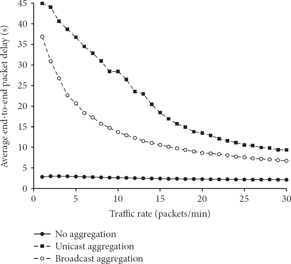
Average end-to-end packet delay.

4.3. Throughput

In Figure 16, the end-to-end throughput of the network is demonstrated. This throughput is expressed as the average number of successful received packets per second per node. We can see at an average traffic rate of 10 packets/min, up to 1.88 packets/min are more received with broadcast aggregation compared with no aggregation and at traffic rate of 12 packets/min, up to 1.59 packets/min are more received with broadcast aggregation compared with unicast aggregation. This is mainly caused by faster transmission and less packet loss.

Figure 16

End-to-end data throughput per node.

4.4. Energy

Figure 17 shows that the total transmit energy consumption with broadcast aggregation can be reduced up to 29% compared with unicast aggregation and up to 71% compared with no aggregation.

Figure 17

Total transmit energy consumption.

From (8) and the values in Table 2, we could calculate that theoretically up to 74% of energy could be saved when broadcast aggregation with $\text{Do}{\text{A}}_{\text{avg}}=\mathrm{5}$ is applied compared with no aggregation. The difference between the theoretical and the actual energy reduction could be explained by the fact that in our simulation $\text{Do}{\text{A}}_{\text{avg}}=\mathrm{5}$ is not reached. Furthermore, we can see that starting from an average traffic rate of 21 packets/min, broadcast aggregation consumes more energy than unicast aggregation. This is because lost packets are not taken into account. Indeed, with unicast aggregation, more packets are lost and since lost packets are not further routed, less energy is consumed than expected.

Table 2

Energy settings.

Parameter	Value
Transmit power	57.42 mW
Listen power	62 mW
Sleep power	1.4 mW
Receive power	62 mW
Beacon size	16 bytes
Beacons per transmission	8
CCA time	0.128 ms
Rx-Tx turnaround time	$2*\mathit{0.192}$  ms

Figures 18 and 19 show, respectively, the total energy consumption and the average energy consumption per successfully delivered packet.

Figure 18

Total energy consumption.

Figure 19

Average energy consumption per successful delivered data packet.

Taking into account the total energy consumption (Figure 18), 27% of energy can be saved compared with no aggregation and up to 13% compared with unicast aggregation. For the no aggregation scenario, we can also see that the total energy consumption stagnates and reaches a maximum because the network becomes congested. For the unicast and broadcast aggregation scenario, this maximum is expected somewhat later.

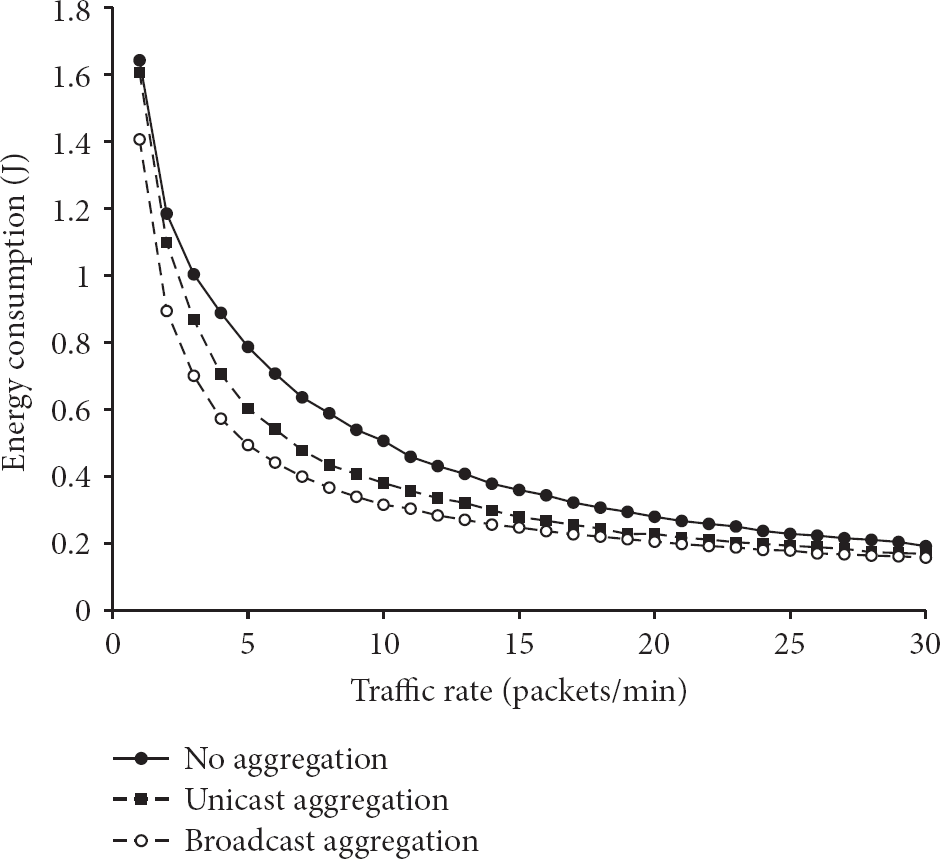
When we take a look at the energy per successfully delivered packet (Figure 19), we can see that up to 38% of energy can be saved compared with no aggregation and up to 19% compared with unicast aggregation.

From the figures, we see that the total energy reduction is much lower than the total transmit energy reduction. The reason can be found in the used MAC protocol and can be seen in Figure 20 that shows the energy distribution of broadcast aggregation in terms of transmit energy, idle listening energy, receive energy, and sleep energy. We can see that much energy is lost due to idle listening.

Figure 20

Total broadcast aggregation energy distribution.

A detailed overview of the energy contributions in Figure 20 can be found in Figures 21 to 23.

Figure 21

Total idle listening energy consumption.

In Figure 21, we can see that the idle listening time reaches a maximum in the no aggregation scenario. This can be explained by the used MAC protocol and the load. First, the number of sent packets increases, so the number of sent beacons also increases and nodes are longer awake. As a consequence, the time spent on idle listening, and thus the resulting energy consumption, increases. However, from a certain point, the time spent on idle listening will decrease since part of this time will be used to transmit/forward/receive the increasing amount of packets. This behavior is also expected for unicast and broadcast aggregation, but since the amount of traffic increases slower since more packets are aggregated, this point will occur at bigger traffic rates.

Figure 22 shows the total receive energy consumption. This is the energy consumed by receiving both beacons and data, even the data that is not destined for this node.

Figure 22

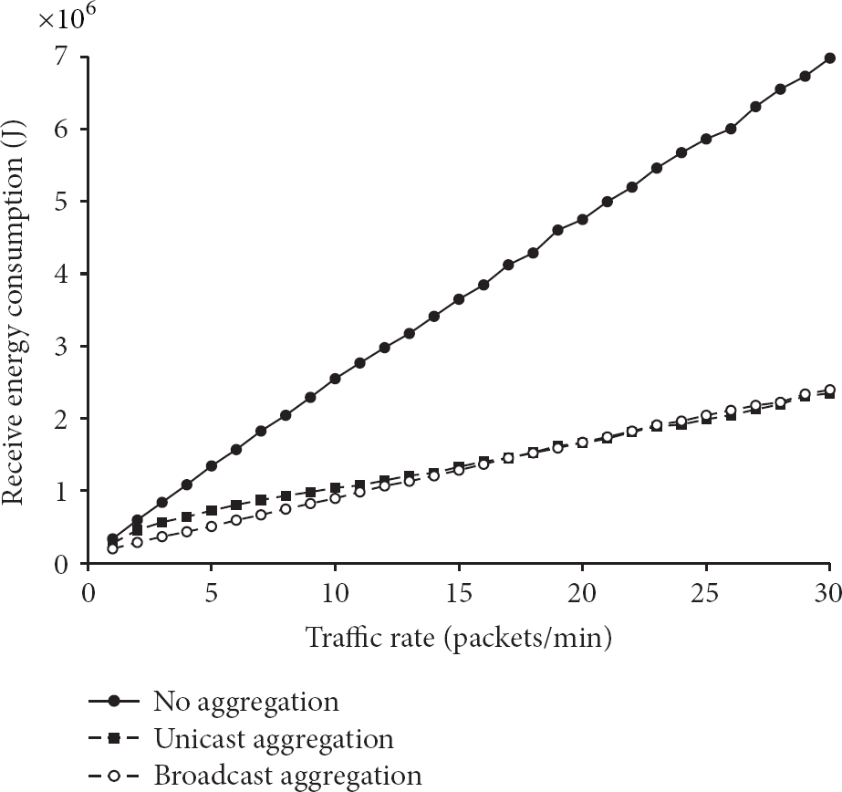
Total receive energy consumption.

Figure 23

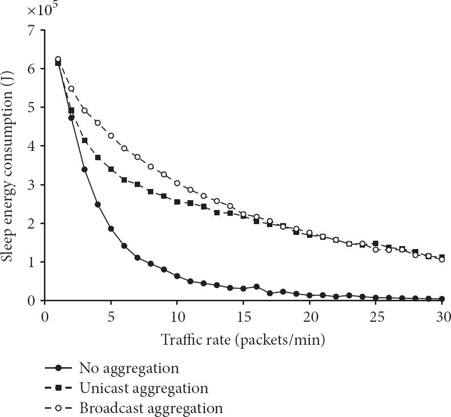
Total sleep energy consumption.

Finally, Figure 23 shows the total amount of energy that is consumed by sleeping. Both from Figures 22 and 23, we can see that broadcast aggregation seems to perform worse than unicast aggregation starting from an average traffic rate of 21 packets/min. This is however not true since lost packets are not taken into account. Unicast aggregation leads to more lost packets which are not routed. This results in less received energy consumption and more sleep energy consumption.

5. Conclusion and Future Work

In-network aggregation is a very efficient way to reduce energy consumption in wireless sensor networks. However, the traditional unicast-based in-network aggregation only works well for source-to-sink traffic. When there are multiple destinations, as is the case in the Internet of Things, aggregation becomes slower, delay increases, reliability drops, and energy consumption increases.

In this paper, we propose to use broadcast aggregation as a solution to overcome these drawbacks. We have shown that broadcast aggregation reduces the average queue occupation with 2 (of the 15 available) places, which leads to fewer packet drops. This leads on its turn to a throughput and reliability increase up to 23% compared with no aggregation and up to 15% compared with unicast aggregation. Moreover, we have shown that packets become less dependent of the individual timeouts per destination which reduces the drawbacks of partial aggregation.

Furthermore we have shown that the average queue delay is decreased by 52% compared with unicast aggregation because aggregation can be performed faster.

Finally, the average DoA is higher, which leads to fewer packets, less overhead, and as a consequence, an energy reduction up to 27% compared with no aggregation and up to 13% compared with unicast aggregation. The overall energy reduction is mainly realized by reducing the transmit energy. Further gains are to be expected by reducing the idle listening energy as well. To this end, several MAC optimizations will be investigated in order to further reduce the energy consumption. For instance, we will investigate the use of destination addresses in the beacon messages, so that nodes that are not the intended receiver can immediately go back to sleep.