RSSI and LQI Data Clustering Techniques to Determine the Number of Nodes in Wireless Sensor Networks

Abstract

With the rapid proliferation of wireless sensor networks, different network topologies are likely to exist in the same geographical region, each of which is able to perform its own functions individually. However, these networks are prone to cause interference to neighbor networks, such as data duplication or interception. How to detect, determine, and locate the unknown wireless topologies in a given geographical area has become a significant issue in the wireless industry. This problem is especially acute in military use, such as spy-nodes detection and communication orientation systems. In this paper, three different clustering methods are applied to classify the RSSI and LQI data recorded from the unknown wireless topology into a certain number of groups in order to determine the number of active sensor nodes in the unknown wireless topology. The results show that RSSI and LQI data are capable of determining the number of active communication nodes in wireless topologies.

1. Introduction

Security maintenance has been a well-studied problem in wireless sensor networks. A wireless sensor network (WSN) is a collaborative network that contains a collection of sensor nodes, each of which has a power source, and is able to individually and autonomously complete the function of discovering and maintaining routing to other sensors through wireless links. Due to these properties, data are collected, processed, and transmitted automatically without any personnel. However, it might give rise to potential security perils during data transmission; for example, “spy” nodes can duplicate the transmitted data and relay it to other wireless topologies without being discovered. In addition, commercial applications apply to such a problem as multiple communication networks can operate in the same frequency ranges, which give rise to interference, errors, and competition.

These security issues often happen when many different wireless topologies locate within the same geographical area. This paper focuses on how to determine the number of “spy” nodes in an unknown network topology. Consider the scenario illustrated in Figure 1. In Figure 1, two networks have been deployed in the same geographical location and have overlapping coverage areas. Hence, they may interfere with one another and cause security issues when operating under the same frequency range, use a common communication protocol, or are directly competing for bandwidth.

Figure 1

Illustration of two networks that have been deployed to the same geographical location and overlap in coverage.

However, in real-world deployment of such networks, the information regarding the overall topology of the network is unknown. To illustrate this we use a coalition network example. That is, as illustrated in Figure 1 the US sensors are unaware that there are British sensors nearby and do not know the number of sensors that have been deployed to the region. The same example can be applied to the commercial sector of two communication companies with coverage over a given city or region. In this paper, we seek to determine the number of nodes as a preliminary study to further determine the topology of the unknown networks without acquiring authentication or encryption. We focus on the use of pattern recognition, clustering, and other classification and identification tools to seek a solution. Firstly, we apply the pattern recognition methodologies commonly used in mathematical morphology (MM) [1–3] known as granulometric size distribution (GSD); secondly, we apply a “bottom up” clustering method known as agglomerative hierarchical clustering (AHC) to build a hierarchy of clusters. Finally, partitioning around medoids (PAM) algorithm otherwise known as K-Medoids clustering technique is used. The primary goal of this paper is to apply these three methods to process the received signal strength indicator (RSSI) and link quality indicator (LQI) data collected from the unknown wireless topology as means to try isolating patterns and determine the number of nodes actively communicating in a network. To the best of our knowledge, it is the first time that clustering techniques are applied to classify RSSI and LQI data for nodes' number information in the research fields.

2. Related Work and Background

RSSI and LQI data is utilized in this paper as two major parameters in wireless sensor networks to apply clustering techniques. These two indicators do not require a priori information regarding the communication protocol and security encryption. These indicators can be observed as the signals are passively collected by a receiver. Hence, if there are inherent patterns associated with the network topology, it is a clear indicator that allows a method to gain insight regarding the unknown network topology.

2.1. RSSI

Received signal strength indicator (RSSI) as the name suggests is a measure of the strength of a received wireless signal. It is obvious that the power of the received signal would decrease with distance. To be precise, power $P_R$ of the received signal is inversely proportional to the square of the distance between the receiver and the transmitter [4]. RSSI can then be defined as the ratio of received power $P_R$ to the reference power $P_{\text{Ref}}$ . Reference power $P_{\text{Ref}}$ is typically taken as 1 mW [5]. In [5], RSSI is defined as

$$\begin{array}{cc}& \text{RSSI}=10·\log \frac{P_{\text{RX}}}{P_{\text{Ref}}},\end{array}$$

(1)

where $P_{\text{RX}}$ is defined as

$$\begin{array}{cc}& P_{\text{RX}}=P_{\text{TX}}·G_{\text{TX}}·G_{\text{RX}}{\left(\frac{\vartheta }{4\pi d}\right)}^2,\end{array}$$

(2)

where $P_{\text{TX}}$ is the transmission power of sender, $P_{\text{RX}}$ is the remaining power of the wave at the receiver, $G_{\text{TX}}$ and $G_{\text{RX}}$ are the gain of transmitter and receiver, respectively, ϑ is the wave length, and lastly d is the distance between the sender and the receiver.

The distance between antennas will directly influence the RSSI value [6, 7]. Hence, RSSI is often used as a tool of localization in wireless sensor networks; please refer to [5, 8–10] as examples of RSSI used in localization of receivers. Localization through RSSI is possible due to the signal attenuation according to the inverse squared rule.

Because of its relationship with distance, ideally RSSI would be a very accurate measure of the receiver's distance from the source. It, however, can get affected from a number of factors such as reflections from objects, electromagnetic fields, diffraction, refraction, and other multipath effects [5]. Due to these effects, only a region of possible location of a sender can be attained. The precision varies and can be improved through proper signal processing techniques and/or characterization of the operating environment.

2.2. LQI

The link quality indicator (LQI) has been used as a substitute to RSSI. LQI represents the quality of the received packet and is not affected as much as the RSSI, by the environment. The LQI represents the number of required retransmissions to receive one radio packet correctly [5]. Basing LQI on the chip error rate and not the strength of the received signal makes LQI perform better than RSSI, since it is not affected drastically by reflections from objects, electromagnetic fields, diffraction, refraction, and so forth. We can see the difference between RSSI data and LQI in Figure 2.

Figure 2

RSSI and LQI data received by the same node.

2.3. Using RSSI and LQI in WSN

As per the definition of RSSI and LQI mentioned above, these two parameters are mostly used for nodes' localization and distance measurement [11–13].

In [14], several measurement-based models including RSSI, time of arrival (TOA), and angle of arrival were described to provide people with statistic models when localizing nodes in cooperative WSNs. Also, Haeberlen et al. [15] designed a system based on probabilistic techniques to localize sensor nodes in an office building by walking around with a laptop recording the observed signal intensities of this building's unmodified base stations. However, to the best of our knowledge, none of these researches have focused on determining the number of nodes by processing RSSI and LQI in WSN.

Instead, we use these two types of parameters to determine if each sensor's information can result in an estimate of its surroundings. In this paper, we seek simple yet effective means to determine the number of participants in the unknown network. Localization methods require more sophisticated methods. We look at the received signals from the unknown topology and use quantitative classification to derive how many nearby nodes could be transmitting at any given point in time, since each sensor is collecting independent information. The estimates should give us insight regarding the number of possible nodes in the unknown topology. Furthermore, since the signal strength is a function of distance, we can determine possible location regions. This results in a geographical estimate of the position of a possible unknown network participant.

This paper is organized as follows. Firstly, we explain the methodology of using GSD functions, AHC, and PAM clustering algorithms, respectively, as means to identify the RSSI and LQI patterns. Secondly, we describe experimental details carried out on a small Zigbee network. Finally, result analysis and conclusion are provided.

3. Methodologies

In this paper, a shape driven clustering technique granulometric size distribution (GSD), a statistical distance clustering approach agglomerative hierarchical clustering (AHC), and a traditional clustering method partition around medoids (PAM) are separately explored to analyze if insight regarding the number of wireless nodes in a nearby network can be determined through collected RSSI and LQI data from sniffer nodes. We employ the GSD, AHC, and PAM methods to separate the patterns of RSSI and LQI from sensor nodes. Accordingly, we developed a real experiment explained in the proceeding section and apply the corresponding tools to generate the results analysis.

3.1. Granulometric Size Distribution

Given the signals of RSSI and LQI, we develop the analysis by employing the granulometric size distribution (GSD) using MM tools. These tools have been fully illustrated through example in [16]. Specifically, we use the GSD method to reduce the dimension of the signal.

The GSD function is generated by continuously using the increasing multiples of structuring elements to probe (remove) the morphological granulometries in the subgraph until all the subgraph area has been diminished. The subgraph area $\text{SG}(f)$ is the area between the curve $f(x)$ and X-axis; structuring elements are kinds of predefined regular shapes, such as a triangle or a rectangle. The MM mentioned in [16] is for the better understanding of the following innovative method called GSD method, because the procedures of generating a GSD function are very similar to the opening operations of the MM theory.

In this paper, a unit square with side length equal to 1 is regarded as the structuring element. The GSD of a signal waveform is denoted as

$$\begin{array}{cc}& \text{GS}{\text{D}}_{\alpha }\left(S\left(t\right)\right)=\frac{\Psi \left(\alpha \right)}{S_0},\end{array}$$

(3)

where $S_0$ is the total subgraph area of the signal waveform. $\Psi (\alpha )$ is the total opening part of the subgraph of that signal waveform, which is defined as

$$\begin{array}{cc}& \Psi \left(\alpha \right)={\displaystyle \sum }_{i=1}^{\alpha }‍\gamma \left(i\right),\end{array}$$

(4)

where $\gamma (i)$ is the opening of a signal waveform $S(t)$ by structuring element $\alpha B$ :

$$\begin{array}{cc}& \gamma \left(\alpha \right)=S_{\alpha B}\left(t\right),\end{array}$$

(5)

where α is a positive integer, which will increase by 1 at each time when opening the signal waveform. B is the structuring element and $\gamma (\alpha )$ is called the trimming area by using α times of B to cut the remaining area of the original waveform. t is the sampling time. According to formula (3), it is clear to see that the pattern spectrum of GSD is a probability distribution according to the definition.

GSD clustering method has been proposed and utilized in several modern researches. In [17], Ayala et al. introduced the concept of granulometric size distribution in detail. In [18], GSD clustering method is adopted to classify the solar radiation patterns of the year. In [16], a new nonparametric method is applied to differentiate signals from noise based on GSD method.

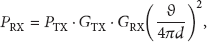
We employ the definitions in [16–18] to generate GSD functions of motifs of the RSSI and LQI signals gathered from an unknown network topology. In Figure 3, an example of GSD function is illustrated. In Figure 3(a), we have a given signal. Then, through the application of the aforementioned definitions, we first generate a stepwise function of the signal with an appropriate base length α, which is illustrated in Figure 3(b). From this stepwise function, we attain a representative GSD function, as shown in Figure 3(c). In this paper, we employ the GSD method to separate the patterns of RSSI and LQI from sensor nodes.

Figure 3

Illustrative example of GSD function.

3.2. Agglomerative Hierarchical Clustering

In this paper, AHC method is utilized to explore if any hierarchical relationship inherently exists inside the RSSI and LQI data, hence allowing derivation of nodes' number. The Hierarchical clustering technique is now a widely used data analysis tool in many applications, such as data mining, statistics, machine learning, spatial database, biology, and marketing strategy [19–21]. In literature [22], Mirkin described the basic concept of AHC clustering method in detail.

We explore AHC to the RSSI and LQI to generate a binary tree (also named “Dendrogram” [22]) derived from the architecture of the data, hoping to directly observe the number of clusters by counting the number of branches of this tree.

Each binary tree has the following characteristics:

• (1)

root node: the whole data set;

(2)

height of the tree: distance between each pair of data points or clusters;

(3)

intermediate nodes: the level to which the objects are closed to each other;

(4)

leaf nodes: corresponding data points;

(5)

clustering criteri: cutting the dendrogram at different levels.

The basic thought procedure of the hierarchical clustering method can be briefly described by the following steps.

Step 1.

Classify each data point into its own singleton cluster.

Step 2.

Each pair of two data points are combined into a single cluster based on closest shortest distance. The distance mainly uses Euclidean distance.

Step 3.

Continuously merge two clusters into one cluster based on closest shortest distance.

Step 4.

Repeat Step 3 until there is only one cluster containing all the points.

Figure 4 shows a binary tree of data. In the binary tree, it is easy to observe that each level of the result is a segmentation of the data and all the data points are successively classified into groups.

Figure 4

A simple example of a binary tree with 30 data points.

In agglomerative clustering, every data point is regarded as its own cluster and pairs of clusters are merged into a bigger cluster until all data points are in one cluster. We use Euclidean distance to calculate the dissimilarities between each RSSI and LQI data pair that are recorded on the same sampling point. Each RSSI and LQI data forms a 2-dimension coordinate: the X-axis is RSSI data and the Y-axis is LQI data. AHC can produce an ordering of object, displaying the data informatively to the researchers. Also, the clusters generated by AHC are relatively smaller [22], which may be helpful for discovery.

3.3. Partitioning Around Medoids

Finally, we apply a traditional clustering algorithm known as PAM to classify the RSSI and LQI data into groups based on the Euclidean distance in order to derive the number of active nodes. PAM is fully described in chapter 2 of Kaufman and Rousseeuw [23]. The purpose of PAM is to find a sequence of targets called medoids, which are centrally placed in clusters. A medoid can be defined as a data point inside a cluster whose average distance (generally using Euclidean distance) to all other data points in the same cluster is minimized [23]. Assume the total number of objects is N and PAM first computes K selected medoids and the number of unselected objects is $Q=N-K$ . The primary goal of the PAM clustering method is to make sure that the average distance of objects to their closest medoid is minimal. PAM has 2 main steps, build and swap [23].

Build. Select a collection of k objects as medoids for an initial set M.

Swap. If the distance or dissimilarity between unselected objects and medoids can be reduced by exchanging a medoid with an unselected object, then the swap step is carried out. The swap step continues until the distance between medoids and unselected objects cannot be reduced any further.

Figure 5 shows a simple example of PAM clustering method, through which the data are classified into 4 groups.

Figure 5

A simple example of PAM clustering result.

Through PAM, we hope to find the various structural features of object, such as the number of medoids (number of groups) which represents the number of clusters and hence the number of active nodes.

Euclidean distance is also used in PAM. Similar to the data format employed in AHC, data pairs are also used as coordinate points, each of which includes one RSSI and one LQI data.

4. Experimental Details

The experiments were conducted using the $TinyOS$ network operating system on $TelosB$ sensor motes. $TelosB$ motes have an 8 MHz TI MSP430 Microprocessor with 10 KB of RAM. The motes have a Chipcon CC2420 radio for wireless communication which is $IEEE\mathrm{802.15.4}/Zigbee$ compliant. The CC2420 radio has programmable power levels. The experiments were run at the default power level of 0 dB and the radio channel was set at 2475 MHz. Experiments were performed indoors. The communication range of the CC2420 radio is approximately 20 m to 30 m indoors and 75 m to 100 m outdoors. In the CC2420, the RSSI value is measured over the first 8 symbols after the start frame delimiter (SFD) of the received physical layer header.

The experimental setup consisted of one node attached to the laptop acting as a base station and three nodes working as sniffers. The sniffer nodes collected the RSSI and LQI values of each packet they overheard from the field nodes and sent this data to the base station. Thus, for each packet transmitted by a field node, the base station had a set of three RSSI and LQI readings from the three sniffers. The experiments were conducted, first, with two field nodes communicating, then with three, and then with four. Each experiment was repeated for three different sizes of the network packet: 10 bytes, 75 bytes, and 115 bytes. In the indoor experiment, distances between the nodes were considerably small. It was assured that no moving objects interfered with the signals. In our experiment, 4 nodes and 3 sniffers are randomly placed. The topology of the nodes in the experiment can be seen in Figure 6.

Figure 6

Node topologies for indoor experiments.

The initial experiment consisted of three sniffers and two field nodes placed in the lab as shown in Figure 6. The two field nodes were routing messages back and forth. Sniffer nodes listened to each radio transmission and collected the RSSI and LQI values of each received packet. The data from all the three sniffer nodes was accumulated at the base station. This experiment was performed for three difference packet sizes, which were 10 bytes, 75 bytes, and 115 bytes. An additional experiment was performed where a third field node was included, with the nodes now communicating in a ring. This configuration was again run for 10 bytes, 75 bytes, and 115 bytes packet sizes and RSSI and LQI data was collected by the sniffers. The last experiment consisted of a fourth additional node and similarly data was collected for this configuration with the three different packet sizes.

5. Result Analysis

5.1. GSD Results

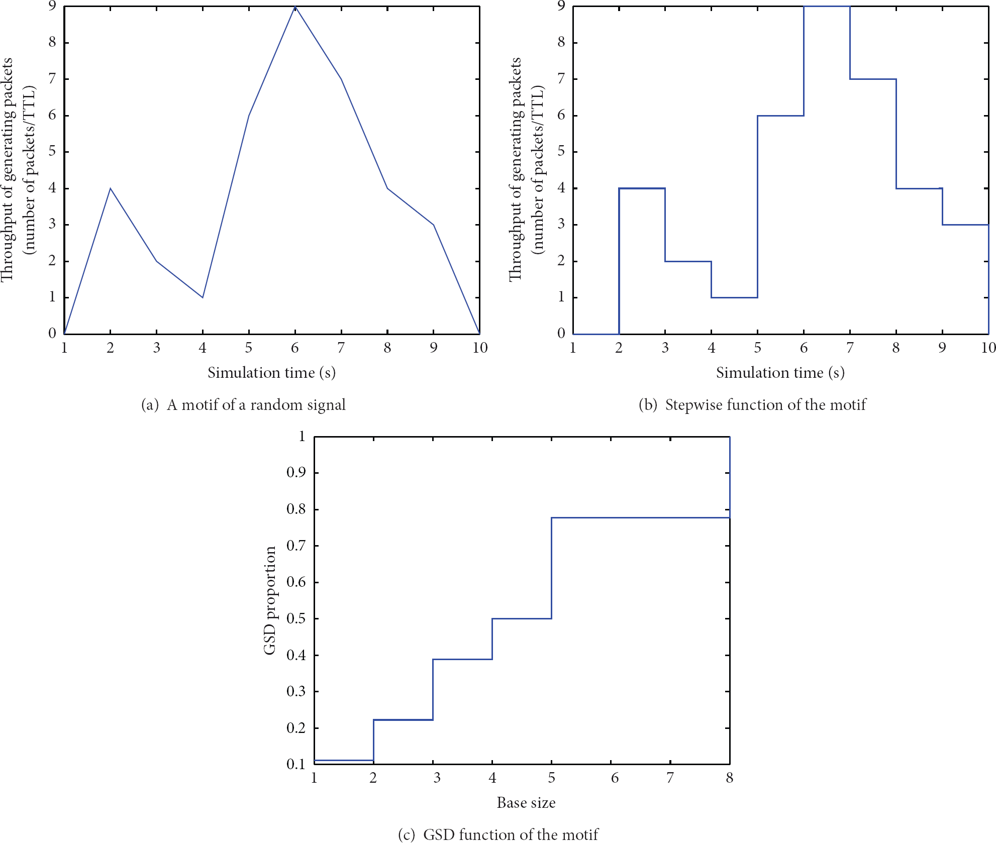
The RSSI and LQI data was converted through the employment of the GSD method. According to the different definition between RSSI and LQI, the corresponding GSD curves are obviously different. Figure 7(a) and Figure 7(b) show the GSD curve of the RSSI and LQI data randomly picked from each sniffer when all 4 nodes are active and communicating with each other.

Figure 7

GSD results of RSSI and LQI.

In Figure 7(a), it is easy to observe that almost all GSD functions of RSSI keep the same low levels, which is flat and close to the X-axis. However, it is very difficult to differentiate them when they are combined together into a single drawing. This is due to the RSSI data being inherently stable according to its mathematical definition and fluctuates narrowly during the entire transmission, while GSD method is a shape driven clustering method and is mostly determined by the shape of the original data.

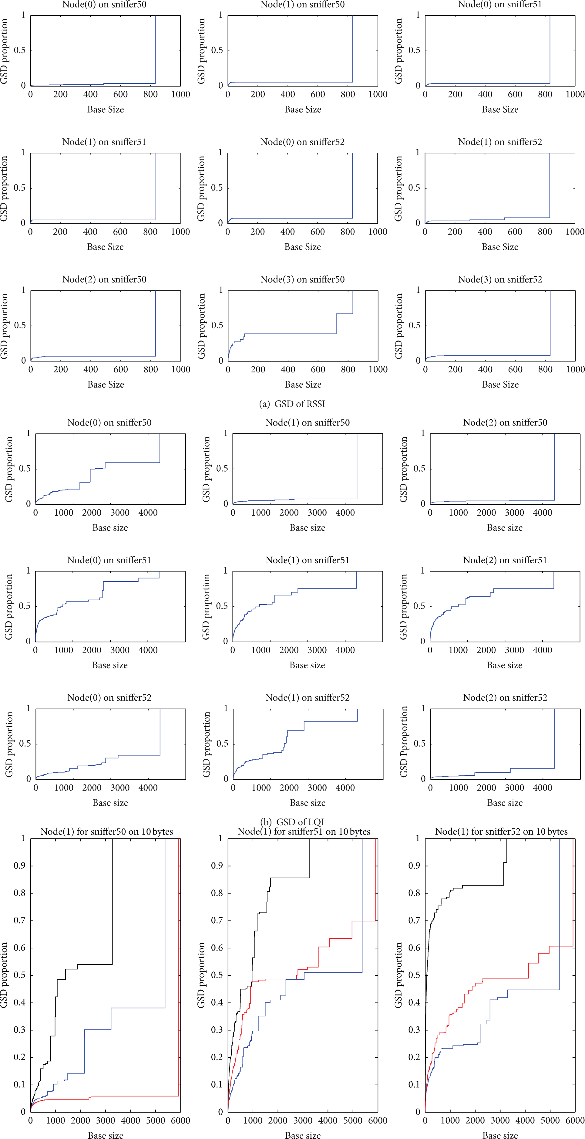
However, in Figure 7(b), the GSD functions of LQI data perform much better than RSSI. Figure 7(b) shows that the GSD functions have more levels and the shape of the GSD functions is dissimilar, which increases the possibility to differentiate them when they are combined together. However, another problem comes when they are combined. Figure 7(c) shows the GSD functions of LQI when combining them together to differentiate them. The blue curves stand for 2 active nodes, the red curves stand for 3 active nodes, and the black curves stand for 4 active nodes, respectively.

The circumstances of different number of active nodes are separated clearly in Figure 7(c). However, they are not consistent for each circumstance and every instance. In most of cases, the 3 curves twist about each other, especially at the beginning of the curves. In other words, it is very hard to draw a linear boundary (a criterion) between each pair of adjacent curves which can clearly divide them. Similarly, the curves also twist each other when using 10 and 115 bytes transmitting packets size. The results of GSD function of LQI are inconsistent, which make it very hard and unclear to determine the number of active nodes. Hence, from the analysis mentioned above, the GSD clustering method is incapable of providing sufficient information of the number of active nodes when classifying RSSI and LQI data.

5.2. AHC Results

Figure 8 shows the dendrogram of agglomerative clustering method when RSSI and LQI data were collected under different circumstances.

Figure 8

AHC results of RSSI and LQI.

From Figure 8, several observations can be made.

•  (1)

Because there are thousands of RSSI and LQI data pairs and each leaf node stands for a data pair, all leaf nodes bunch up together so that it is impossible to know which data pair is classified into which cluster. At the bottom of each figure, where it would be desirable to clearly show the data points, the data points are now bunching up together and become several bold lines.

 (2)

The numbers of clusters are determined by cutting the trees at appropriate levels. However, from Figure 8, it is difficult to come up with a method or criteria to determine where the dendrogram should be cut. Hence, it is unclear how to find an appropriate height level where the trees can be cut to obtain the number of clusters.

 (3)

The intermediate nodes in hierarchical binary tree provide no information about how many clusters there are after classification.

Due to the reasons presented above, it is concluded that RSSI and LQI data are incapable of providing sufficient information about the number of active nodes in an unknown wireless topology when applying the agglomerative clustering technique. Agglomerative clustering method is incapable of classifying the data. Hence, it is unable to provide enough information with regard to how many nodes are communicating in an unknown wireless topology.

5.3. PAM Results

PAM clustering results will be shown in clustering plots. A clustering plot is a two-dimensional coordinate axis. Each data pair (RSSI, LQI) is mapped to the coordinate axes. The X-axis represents RSSI and the Y-axis represents LQI. Figure 9 shows some PAM clustering results. The results from different circumstances are described as (number of active nodes)_(transmitting packets size)_(sniffer that data received). For example, $2\_10\_50$ means the RSSI and LQI received by sniffer 50 when two nodes are communicating simultaneously using 10-byte packet size.

Figure 9

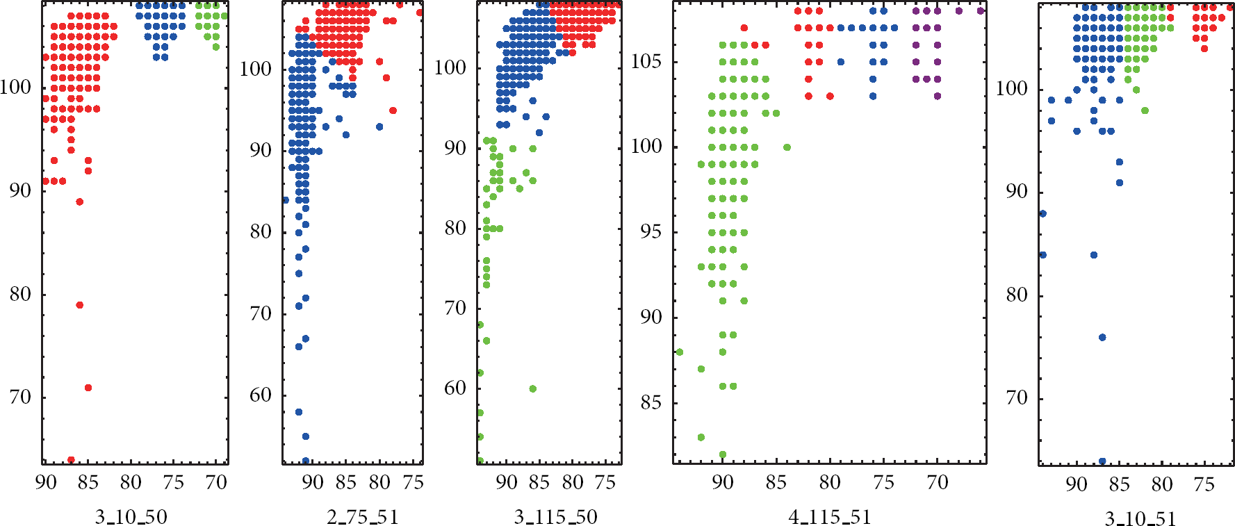
PAM results of RSSI and LQI.

In Figure 9, it is observed that the number of clusters that PAM classified equals the number of active sensor nodes that are placed in the unknown wireless topology. Each color stands for a cluster. The number of data in each cluster is tabulated in Table 1. The results in Table 1 show that the number of data points in each cluster is almost equal to the average data number of the entire data, which means that the clustering results are very reasonable.

Table 1

Number of data in each cluster.

	3_10_50	2_75_51	3_115_50	3_10_51	4_115_51
Cluster1	1334	2011	1289	1337	999
Cluster2	1332	1989	1348	1357	1006
Cluster3	1334		1373	1306	995
Cluster4					1000

However, not all results under different circumstances are consistently correct. In some cases, the number of clusters is less than the number of active nodes. The clusters that contain more nodes need to be further clustered in order to obtain more accurate results. In other cases, the number of clusters is more than the number of active nodes. In these cases, some clusters contain only a few nodes, which are obviously less than other clusters, can be regarded as bad clusters, and need to be excluded. These clusters are generated due to the noise or interference during transmission. All PAM results are shown in Table 2. In Table 2, there are 16 correct clustering results in the total 27 circumstances; the rate of accuracy is 59%. The results show that although it is not completely reliable, PAM clustering method is indeed usable to classify the data into corresponding number of groups.

Table 2

PAM clustering results.

Receiver	Sniffer0
Number of nodes	2			3			4
Packets size (bytes)	10	75	115	10	75	115	10	75	115
Clustering results	3	4	2	3	2	3	2	2	3
Further processing results	2	2	*	*	3	*	4	6	4
Receiver	Sniffer1
Number of nodes	2			3			4
Packets size (bytes)	10	75	115	10	75	115	10	75	115
Clustering results	2	2	13	3	2	2	2	2	4
Further processing results	*	*	2	*	3	5	2	3	*
Receiver	Sniffer2
Number of nodes	2			3			4
Packets size (bytes)	10	75	115	10	75	115	10	75	115
Clustering results	3	3	5	3	4	2	1	2	7
Further processing results	2	3	5	*	4	4	1	3	3

${}^{\mathrm{*}}$ No need to be further processed.

6. Conclusion

In this paper, a practical network problem in WSN is presented. Different kinds of clustering mechanisms are proposed as means to classify the RSSI and LQI data, which is generated by the corresponding sensor nodes in the adjacent wireless network when they are transmitting simultaneously. RSSI is a distance based network parameter, which is a parameter to measure signal strength, while LQI is a metric of the link quality of the received signal. Experiments and literature prove that LQI data fluctuate very dramatically and frequently during transmission. Neither RSSI nor LQI are security parameters and both of them are easily recorded and collected.

Three different clustering techniques are applied to analyze the RSSI and LQI data to explore their inherent characteristics, from which information can be obtained about the number of active nodes in a nearby unknown wireless topology. Corresponding clustering results are shown in this paper. Finally, PAM is capable of classifying the RSSI and LQI data. This implies that, in a wireless network, RSSI and LQI generated by sensor nodes indeed contain information of how many nodes are transmitting data simultaneously in that wireless network. These results were found by unsupervised classification. Although PAM clustering method performs better than GSD and hierarchical agglomerative clustering method, its results are not reliably correct. Future research should explore other clustering methods that perform better than PAM clustering method.