Localization Algorithms in Large-Scale Underwater Acoustic Sensor Networks: A Quantitative Comparison

Abstract

Recently underwater acoustic sensor networks (UASNs) have drawn much attention because of their great value in many underwater applications where human operation is hard to carry out. In this paper, we introduce and compare the performance of four localization algorithms in UASNs, namely, distance vector-hop (DV-hop), a new localization algorithm for underwater acoustic sensor networks (NLA), large-scale hierarchical localization (LSHL), and localization scheme for large scale underwater networks (LSLS). The four algorithms are all suitable for large-scale UASNs. We compare the localization algorithms in terms of localization coverage, localization error, and average energy consumption. Besides, we analyze the impacts of the ranging error and the number of anchor nodes on the performance of the localization algorithms. Simulations show that LSHL and LSLS perform much better than DV-hop and NLA in localization coverage, localization error, and average energy consumption. The performance of NLA is similar to that of the DV-hop. The advantage of DV-hop and NLA is that the localization results do not rely on the number of anchor nodes; that is, only a small number of anchor nodes are needed for localization.

1. Introduction

Oceans cover about 71% of the Earth's surface, but most of them have not been explored up to now. Recently, there has been a growing interest in ocean exploration activities [1]. UASNs have been widely applied in many fields, such as naval defense, environmental pollution monitoring, earthquake or tsunami forewarning, and ocean life monitoring systems. Sensor nodes are deployed both underwater and on the water surface covering the entire monitored space to cooperatively fulfill monitoring tasks. In all applications, localization is a fundamental and significant task in UASNs.

Although localization in terrestrial wireless sensor networks (TWSNs) has been well studied up to now, localization in UASNs is still a challenging problem due to the following reasons [2]: (I) unavailability of global positioning system (GPS); (II) low bandwidth, long delay, and high bit error rate of underwater acoustic links; (III) necessity of large number of sensor nodes to cover wide and deep oceanographic regions. What is more, some uncontrollable factors such as the mobility caused by water current and oceanographic animals bring a new set of challenges to localization in UASNs.

Sensor nodes in the network can be classified into two categories according to whether they know their positions, namely, anchor node (beacon node) and ordinary node (unknown node). Anchor nodes are those who can directly get their absolute positions from GPS or by other means. Ordinary nodes are those who can communicate with anchor nodes to estimate their own positions using localization algorithms.

Recently many localization algorithms for WSNs and UASNs have been proposed [3–6]. The authors classify localization algorithms into two categories [7]: range-based algorithms and range-free algorithms. The former contains the protocols which calculate locations of unknown nodes by estimating absolute point-to-point distances or angles, while the latter makes no assumption about the availability or validity of such range information. Although range-based schemes can provide more accurate position estimations, they need additional hardware for distance measurement, which leads to the increase in the network cost correspondingly. Relatively, range-free schemes do not need additional hardware support. However, range-free schemes can only provide coarse position estimations. Localization algorithms also can be classified into distributed and centralized [8]. In distributed algorithms, each unknown node plays a part in localization information collection and runs a distance estimation algorithm individually. On the contrary, in centralized localization algorithms, a central unit is responsible for estimating the location of each unknown node, which will be bound to increase the burden of the central unit and reduce the lifetime of the whole networks. Experiments show that distributed localization protocols are more effective for large-scale UASNs.

The main contribution of this paper is that we introduce and compare the performance of four distributed localization algorithms which are suitable for large-scale UASNs. The schemes are distance vector-hop (DV-hop), a new localization algorithm for underwater acoustic sensor networks (NLA), large-scale hierarchical localization (LSHL), and localization scheme for large-scale underwater networks (LSLS). We use MATLAB as the simulation tool and compare the performance of the algorithms in terms of localization coverage, localization error, and average energy consumption. To compare the algorithms more comprehensively, we analyze the impacts of the ranging error and the number of anchor nodes on the performance of the localization algorithms.

The remainder of the paper is organized as follows. Section 2 summarizes the related works in UASNs. Section 3 describes DV-hop, NLA, LSHL, and LSLS algorithms in detail. Section 4 presents a detailed analysis of simulation results. Section 5 draws conclusions and summarizes contributions.

2. Related Work

As mentioned above, localization in UASNs faces some unavoidable challenges. Global positioning system (GPS) is commonly used in TWSNs, while it is impractical in UASNs since GPS signals cannot propagate in water. Radio signal propagates at long distances through water only at extra low frequency between 30 Hz and 300 Hz, which requires long antennae and high propagation power [8]. Moreover, the variable speed of sound and the node mobility caused by water current aggravate new challenges to localization issues in UASNs.

Due to the challenges mentioned above, localization algorithms in UASNs should be specifically designed. Experiments show that acoustic signal attenuates less and travels further in the water. Thus, acoustic communication is assumed to be the most promising mode for underwater communication. Both range-based algorithms and range-free algorithms have their own advantages and disadvantages. We will overview some representative range-based and range-free localization algorithms in Sections 2.1 and 2.2, respectively.

2.1. Range-Based Algorithms

Othman et al. proposed a node discovery and localization protocol (NDLP) for UASNs [9, 10]; it is an anchor-free and range-based localization method. Localization begins with a node discovery phase by a seed node, which is aware of its self-position and selects other seeds iteratively. Seed nodes are responsible for assisting the other nodes with localization. Large scale of unknown nodes can be localized by selecting seed nodes continuously. However, the node discovery phase will spend much time and consume more energy, since each node participates in message exchange in order to select the seed nodes. What is more, in sparse sensor networks, it is possible that no sensor node can be selected as seed nodes, which will result in failure of localization.

Mirza and Schurgers aim at solving the localization problem in mobile UASNs by using a centralized localization technique, called collaborative localization scheme (CLS) [11]. In CLS, sensor nodes collaboratively determine their positions without using long range transponders which are equipped on surface buoys or ships. Starting at the ocean surface where the network is deployed, sensor nodes use buoyancy control to descend deeper into the ocean. Once a maximum desired depth is reached, the sensor node travels back to the ocean surface. While sensor nodes are descending, although they can calculate their depths by using pressure sensors, their positions in the other two dimensions are changing continuously with water current, which cannot be estimated. CLS is an anchor-free and cost effective strategy. The main drawback of CLS is that the localization results depend highly on network architecture. Besides, the performance of CLS will be seriously affected in sparse and heterogeneous networks.

Isik and Akan proposed a localization algorithm called three-dimensional underwater localization (3DUL) [12]. 3DUL algorithm can achieve network wide robust 3D localization by using a distributed and iterative algorithm. It is emphasized that 3DUL algorithm exploits only three surface buoys for localization initially. 3DUL algorithm requires that sensor nodes in the network should be equipped with conductivity, temperature, and depth (CTD) sensors to estimate the sound speed. The depth information is also used for the projection of the anchor nodes. Generally speaking, 3DUL contains two phases. During the first phase, unknown nodes estimate their distances to neighboring anchor nodes. In the second phase, unknown nodes use these pair wise distances and depth information to project the anchor nodes onto their horizontal levels and form virtual geometric structures. If the structure is robust, the unknown node locates itself by using dynamic trilateration method and upgrades to be an anchor node to assist other unknown nodes in localization. This process dynamically repeats to localize as many nodes as possible. Simulations show that the 3DUL algorithm can achieve relatively high accuracy in UASNs.

2.2. Range-Free Algorithms

Chandrasekhar and Seah hold the view that, for large-scale UASNs, obtaining the exact location of each unknown node may be infeasible [13]. Therefore, they proposed a range-free algorithm called area localization scheme (ALS) to achieve localization. It is notable that ALS estimates the position of each unknown node within a certain area rather than its exact location. In ALS, anchor nodes are responsible for sending out signals under different levels of power to localize unknown nodes. Unknown nodes simply listen to the signals and record the anchor nodes’ IDs and their corresponding power levels. Then the collected data and the recorded information are sent to the sink node, which is able to draw out the map of areas divided by all the anchor nodes’ transmitting signals and localize the unknown nodes. ALS is a range-free localization algorithm without synchronization requirement. However, since ALS is a coarse localization scheme, it is not suitable for accurate localization and instant information gathering.

Ma and Hu proposed a maximum-likelihood source localization approach (MLSL) for UASNs [14]. Sensor arrays are used during localization and each sensor node is equipped with an array. Sensor nodes are attached to the sensor arrays via wire connections. Each target which waits to be localized periodically emits a narrow-band acoustic signal. Sensor nodes which have received the signal can obtain the target locations and signal amplitudes by using the negative log-likelihood function. The maximum likelihood estimation of the target location is obtained based on the global likelihood function, which is the sum of the local likelihood function. MLSL approach does not require distance measurement and time synchronization. It is analyzed that computation overhead of sensor nodes and targets is low, while communication overhead and energy consumption are high, as all the local likelihood functions are forwarded to a fusion center. MLSL is not suitable for large-scale UASNs due to the fact that sensor nodes are attached to the sensor arrays via wire connections and global wireless network architecture.

Range-based localization algorithms can achieve relatively high accuracy in theory. However, they need additional hardware and time synchronization, which increases the cost of UASNs. Therefore, range-free localization algorithms are more popular in real applications, especially when the network does not require high localization accuracy. In range-free algorithms, neighboring distances or angle information cannot be acquired due to hardware limitation. Thus, there should be trade-off among localization performance evaluation metrics, such as localization accuracy, energy consumption, and convergence speed, depending on the application requirements. Only by being familiar with the characteristics of different kinds of localization algorithms and their application occasions can we propose novel algorithms with better performance and efficiency for UASNs in the future. In this paper, we choose LSHL and LSLS as representative range-based algorithms and NLA and DV-hop as representative range-free algorithms. To compare the four algorithms in a more comprehensive and fair way, the two algorithms which we choose under the same category have similar localization mechanisms. Next we will analyze and compare the performance of the four localization algorithms in detail.

3. Distributed Localization Algorithms for Large-Scale UASNs

In this section, we introduce four localization algorithms which are suitable for large-scale UASNs. DV-hop and NLA are range-free localization algorithms; LSHL and LSLS are range-based algorithms.

3.1. DV-hop Algorithm

The DV-hop is a classic localization algorithm [15, 16]. The algorithm consists of three subphases. Firstly, unknown nodes will compute the least hop counts to each anchor node. Secondly, shortest hop-length between an unknown node and an anchor node can be calculated. Then, the distances between unknown nodes and anchor nodes can be computed correspondingly. Finally, unknown nodes will calculate their positions by using trilateration method.

Now we will introduce the DV-hop localization algorithm in detail. The three subphases of the DV-hop localization algorithm are as follows.

(a) Computing the Least Hop Counts. Each anchor node sends its information to its neighboring nodes by broadcasting message packages. The message package includes identifier ID, its coordinates, and hop count $H_i$ , where the initial value of $H_i$ is zero. Each sensor node which receives message packages will save these pieces of information as a vector; then it will transmit the information to its neighboring nodes and increase $H_i$ by one. When a sensor node receives a message package from the same ID, the sensor node will compare the received $H_i$ with the existing $H_i$ . If the new value is smaller than the old one, it means there is a shorter path to the same anchor node; then, the old $H_i$ will be replaced by the new one. Otherwise, the sensor node will discard this message package and stop transmitting the information to its neighboring nodes. By this propagation method, unknown nodes in the networks can calculate the least hop counts to each anchor node.

(b) Estimating Distances among Sensor Nodes. After step (a), each sensor node saves the coordinates of all the anchor nodes and the least hops to the anchor nodes. Thus, each anchor node can calculate the one-hop distance. The average of one-hop distances can be computed by the following formula:

$$\begin{array}{cc}& \text{One-Ho}{\text{p}}_i=\frac{{\sum }_{j\ne i}\sqrt{{\left(x_i-x_j\right)}^{\mathrm{2}}+{\left(y_i-y_j\right)}^{\mathrm{2}}+{\left(z_i-z_j\right)}^{\mathrm{2}}}}{{\sum }_{j\ne i}{h}_i},\end{array}$$

(1)

where $(x_i,y_i,z_i)$ and $(x_j,y_j,z_j)$ are coordinates of anchor node i and j, respectively. $h_i$ is the hop count between anchor nodes i and anchor node j. Each anchor node broadcasts the one-hop distance in the network. Unknown nodes receive and save the first arriving one-hop distance information. At the same time, they transmit the one-hop distance to their neighboring nodes.

At the end of this phase, unknown nodes will calculate distances to all the anchor nodes by the following formula:

$$\begin{array}{cc}& d_i=\text{One-Ho}{\text{p}}_i\times H_i.\end{array}$$

(2)

(c) Computing the Locations of Unknown Nodes. Since unknown nodes have already known their distances to each anchor node and the coordinates of the anchor nodes, the unknown nodes can calculate their coordinates by using the multilateration method.

Generally speaking, DV-hop is a relatively simple localization algorithm to realize. However, unknown nodes use multihop anchor nodes to help in localization, which will result in big localization error during localization process.

3.2. NLA Algorithm

Famoori and Javida proposed the NLA for underwater acoustic sensor networks [17]. Firstly, the authors introduced the ad hoc positioning system (APS) algorithm. APS is a distributed and connectivity-based localization algorithm which estimates locations of unknown nodes with the support of at least four anchor nodes. Each anchor node propagates its location to all the other sensor nodes in the network using the concept of distance vector (DV) exchange, where sensor nodes in a network periodically exchange their routing tables with their one-hop neighboring nodes. When an anchor node obtains distances to other anchor nodes, it will calculate an average one-hop count (called the correction factor), which is then propagated throughout the network. The correction factor $c_i$ of anchor i is calculated by the following formula:

$$\begin{array}{cc}& c_i=\frac{{\sum }_{j\ne i}\sqrt{{\left(x_i-x_j\right)}^{\mathrm{2}}+{\left(y_i-y_j\right)}^{\mathrm{2}}+{\left(z_i-z_j\right)}^{\mathrm{2}}}}{{\sum }_{j\ne i}{h}_i}.\end{array}$$

(3)

Since the unknown nodes have already known the locations of the anchor nodes and the correction factors, they are able to estimate their own locations like the way the DV-hop algorithm does. Once a sensor node receives a correction factor, it will ignore the others to ensure that each sensor node only uses one correction factor. As shown in Figure 1, S is an unknown node and $A_{\mathrm{1}}$ , $A_{\mathrm{2}}$ , $A_{\mathrm{3}}$ , and $A_{\mathrm{4}}$ are anchor nodes. Assume that the correction factors of $A_{\mathrm{1}}$ , $A_{\mathrm{2}}$ , $A_{\mathrm{3}}$ , and $A_{\mathrm{4}}$ are $c_{\mathrm{1}}$ , $c_{\mathrm{2}}$ , $c_{\mathrm{3}}$ , and $c_{\mathrm{4}}$ , respectively. Since $A_{\mathrm{3}}$ is the closest anchor node to S, according to ASP, distances between S and the four anchor nodes are $\mathrm{3}\times c_{\mathrm{3}}$ , $\mathrm{2}\times c_{\mathrm{3}}$ , $\mathrm{1}\times c_{\mathrm{3}}$ , and $\mathrm{3}\times c_{\mathrm{3}}$ , respectively.

Figure 1

An example of ASP localization.

Since the average of the distances between unknown nodes and anchor nodes is presented as an average distance, the average distance is not accurate, which will result in inaccuracy in coordinates estimation of the unknown nodes. Authors then proposed a new algorithm to improve the localization performance of the APS algorithm by creating a neural network. The new method solves the localization problem by creating a neural network using the received data from anchor nodes, so a general map of the sensor nodes’ positions is estimated by this way. This method uses neural network to estimate the positions of the unknown nodes. In short, the neural network is divided into several areas according to the communication range of the anchor nodes. Each unknown node knows which area it belongs to. Then each unknown node will compute its distance to the anchor nodes around.

In this paper, to compare NLA and DV-hop algorithms, we use the multilateration method to calculate the coordinates of unknown nodes.

3.3. LSHL Algorithm

Zhou et al. presented the LSHL algorithm for UASNs [18]. Figure 2 shows the network architecture of the LSHL algorithm. There are three types of sensor nodes in the network, surface buoys, anchor nodes, and ordinary nodes. Surface buoys are those who drift on the water surface and can get their absolute locations from GPS or by other means. It is assumed that surface buoys can always get accurate location information. Anchor nodes can directly communicate with the surface buoys in order to get their positions and they also can communicate with ordinary nodes and help them in localization. Ordinary nodes can only communicate with the anchor nodes to locate themselves.

Figure 2

A typical underwater sensor network setting.

A hierarchical localization approach is proposed to handle the large-scale UASNs. The researchers divided the whole localization process into two subprocesses: anchor node localization process and unknown node localization process. Experimental results show that, with advanced signal processing technologies, most of these anchor nodes can obtain their accurate positions even for mobile underwater environment. Thus, they pay more attention to unknown node localization, for which they propose a distributed range-based scheme, which combines a 3D Euclidean distance estimation method with a recursive location estimation method.

During the unknown node localization process, there are two types of nodes: reference nodes and nonlocalized nodes. In the initialization phase, all anchor nodes label themselves as reference nodes and set their confidence values to 1. All the ordinary nodes are nonlocalized nodes. Each reference node periodically broadcasts a beacon message, containing its ID. All the neighboring nodes which receive this beacon message can estimate their distances to this reference node using measurement techniques. Each nonlocalized node contains a counter m, which represents the number of the reference nodes that it knows distances to, and a counter n, which represents the number of the localization messages that it broadcasts.

Once the localization process begins, each nonlocalized node keeps checking m. If $m<4$ , the nonlocalized node broadcasts a localization message which contains all the received coordinates of the reference nodes and its estimated distances. Otherwise, the nonlocalized node will use three-dimensional Euclidean distance estimation to estimate distances to more nonneighboring reference nodes. After this step, m is increased and the nonlocalized node returns to the m-checking phase. Until $m\ge \mathrm{4}$ , then, the nonlocalized node will select four reference nodes with the highest confidence values to calculate its coordinates. After the calculation, the nonlocalized node will compute its trust value η. If η is larger than or equal to the trust threshold λ, the nonlocalized node becomes a new reference node. Otherwise, it remains to be a nonlocalized node.

The location error δ and confidence value η are calculated by the following formulas:

$$\begin{array}{cc}& \delta =\sum _i\left|{\left(u-x_i\right)}^{\mathrm{2}}+{\left(v-y_i\right)}^{\mathrm{2}}+{\left(w-z_i\right)}^{\mathrm{2}}-l_i^{\mathrm{2}}\right|\\ \eta =\{\begin{array}{cc}\mathrm{1}\hfill & \left\{\text{if}\hspace{0.17em}\text{node}\hspace{0.17em}\text{is}\hspace{0.17em}\text{the}\hspace{0.17em}\text{initial}\hspace{0.17em}\text{anchor}\right\}\hfill \\ \mathrm{1}-(\phantom{{+{\left(w-z_i\right)}^{\mathrm{2}}\phantom{\sum _i‍})}^{-1}}\delta \times (\sum _i‍{\left(u-x_i\right)}^{\mathrm{2}}\hfill & \hfill \\ \hspace{1em}\hspace{1em}\hspace{1em}\hspace{1em}\hspace{1em}+{\left(v-y_i\right)}^{\mathrm{2}}\hfill & \hfill \\ \hspace{1em}\hspace{1em}\hspace{1em}\hspace{0.5em}\hspace{0.17em}\hspace{0.17em}\hspace{1em}{+{\left(w-z_i\right)}^{\mathrm{2}}\phantom{\sum _i‍})}^{-1})\hfill & \left\{\text{others}\right\},\hfill \end{array}\end{array}$$

(4)

where $(u,v,w)$ are the estimated coordinates of the unknown node, $(x_i,y_i,z_i)$ are the coordinates of the reference node i, and $l_i$ is the measurement distance between the unknown node and node i.

3.4. LSLS Algorithm

Cheng et al. presented the LSLS algorithm for UASNs [19]. Similar to LSHL algorithm, any successfully localized node can become reference node to help in localization in LSLS algorithm, if its trust threshold value is larger than or equal to the trust threshold.

The LSLS algorithm is based on a basic time synchronization free localization (BSFL) algorithm. The BSFL algorithm is a general localization method that will work as long as the three anchors are not collinear. However, it can only be applicable to sensors that reside in the feasible space of three anchors that can mutually hear each other. The LSLS algorithm utilizes the BSFL algorithm as a prime method to localize large-scale underwater networks while retaining the nice features of the BSFL algorithm such as free time synchronization.

The LSLS includes three phases, sea surface anchor localization phase, iterative localization phase, and complementary phase. In the first phase, three surface anchors in communication range send their beacon messages sequentially as described in the BSFL algorithm. Figure 3 shows an example of the projection technique. A, B, C are anchor nodes; S is an unknown node. A, B, C project the three beacons onto the horizontal plane containing S. Then, trilateration is performed to transform these range estimates into coordinates. Thus, it successfully transforms 3D underwater localization problem into a problem of localizing an unknown node in a horizontal plane with the projection technique.

Figure 3

An example of projection technique.

In the second phase, once an unknown node is localized, it can become an active node and join the process of anchor group construction. The selection of new reference nodes and the localization procedure are repeated iteratively. The iterative phase of selecting the new reference nodes is similar to that of the LSHL algorithm. The difference between the two algorithms is that, at each round, the LSLS algorithm chooses as small number of reference nodes as possible, so that most of the nodes are still passive. In addition, the authors also provided an anchor selection strategy to maximize the coverage overlap among the three new anchors.

In the third phase, if an unknown node fails to be localized in the first two phases, it will send a location request. A new group of anchors will then be selected to localize the unknown nodes. To preserve communication overhead, the selected groups of anchors should cover as large to-be-localized area as possible. Then the unknown nodes that are covered by the elected anchor group localize themselves by using BSFL algorithm.

4. Performance Analysis and Comparison

In this paper, we use MATLAB to simulate the performance of DV-hop, NLA, LSHL, and LSLS algorithms. We compare the localization algorithms in terms of localization coverage, localization error, and average energy consumption. Besides, we analyze the impacts of the ranging error and the number of anchor nodes on the performance of the localization algorithms. In simulations, sensor nodes are randomly deployed in a 500 m * 500 m * 500 m monitored space and all the nodes in the network are assumed to be stationary.

Localization coverage is defined as the ratio of the localizable ordinary nodes to the total number of ordinary nodes. Localization error is the average distance between the estimated positions and the real positions of the ordinary nodes. Average energy consumption is defined as the overall energy consumption in the network which is divided by the number of the localizable ordinary nodes.

In our simulations, we design two groups of experiments for each evaluation criterion. In the first group, we change the communication range of the nodes from 95 m to 130 m with a step of 5 m while keeping the number of nodes 500 which include 100 anchor nodes and 400 unknown nodes. In the second group, we change the number of nodes from 500 to 800 with a step of 50 while keeping the communication range 100 m. We take the average of 50 simulation runs as the final results to reduce accidental errors. The simulation results are displayed as follows.

4.1. Localization Coverage

From Figure 4, we can observe that, with the increase of communication range, the average localization coverage of LSHL and LSLS algorithms increases slowly and they have much higher localization coverage than NLA and DV-hop algorithms. For the LSHL, when communication range changes from 95 m to 100 m, localization coverage increases significantly. After that, it performs almost the same as the LSLS algorithm. When the communication range is relatively small, localization coverage of the LSLS is larger than that of the LSHL, due to the fact that the LSLS transforms 3D localization problem into 2D localization problem with projection technique. In other words, only three anchor nodes are needed to localize an unknown node, which contributes to the improvement of localization coverage. The NLA algorithm has slightly higher localization coverage than the DV-hop algorithm because different correction factors are used to estimate the distances between anchor nodes and unknown nodes in the NLA, while the DV-hop just chooses the closest anchor nodes’ correction factors. Since NLA and DV-hop algorithms use multihop anchor nodes to help in localization, the localization errors are relatively larger than those of LSHL and LSLS algorithms, which results in the decrease in localization coverage.

Figure 4

Localization coverage with varying communication ranges.

It can be observed from Figure 5 that, with the increase in the number of nodes, localization coverage of NLA and DV-hop algorithms does not change obviously and their localization coverage is much smaller than that of the other two algorithms. For NLA and DV-hop algorithms, although large number of nodes can be localized, the estimated positions are not accurate. The localization coverage of NLA and DV-hop algorithms is quite low and not influenced by the number of nodes significantly. For LSHL and LSLS algorithms, localization coverage increases with the increase in the number of nodes and their localization coverage maintains high, because when more nodes are deployed in the network, anchor nodes can help more ordinary node with localization, which increases localization coverage. In addition, when the number of ordinary nodes is 500, since localization coverage of LSHL and LSLS algorithms has already reached high values, when the number of nodes continues to increase, localization coverage will not increase prominently.

Figure 5

Localization coverage with varying number of nodes.

4.2. Localization Error

Figure 6 depicts the relationship between the localization error and the communication range. For LSHL and LSLS algorithms, localization errors decrease slowly with the increase of communication range. It is reasonable that, with the increase of communication range, more ordinary nodes can be localized by anchor nodes instead of reference nodes, which can improve localization accuracy. For NLA and DV-hop algorithms, localization errors vary up and down with the increase of communication range. On the one hand, when communication range is relatively small, one-hop distance estimation is not accurate. On the other hand, with the increase of communication range, more anchor nodes could play a part in one-hop distance estimation, which also may increase estimation errors.

Figure 6

Localization error with varying communication ranges.

Figure 7 describes the relationship between the localization errors and the number of nodes. For NLA and DV-hop algorithms, localization errors decrease with the increase of the number of nodes. This is because that, when the number of anchor nodes is the same, the increase of the number of nodes will not change the correction factors so the localization error does not change significantly. For LSHL and LSLS algorithms, localization errors increase with the increase of the number of nodes, because more ordinary nodes can be localized by reference nodes rather than anchor nodes, which results in accumulating errors. However, the increase of the ordinary nodes provides more choices to select reference nodes with relatively higher trust values, which can improve localization accuracy to some extent. Therefore, the increase of the localization errors is not prominent.

Figure 7

Localization error with varying number of nodes.

4.3. Average Energy Consumption

Figure 8 presents the relationship between the average energy consumption and different communication ranges. Simulations show that the average energy consumption of NLA and DV-hop algorithms does not change with the communication range, because the message packages of the two algorithms in the network keep the same, no matter whether the ordinary nodes can be localized. Thus, once the number of ordinary nodes is decided in the network, the average energy consumption does not change. The average energy consumption of NLA and DV-hop algorithms is higher than that of LSHL and LSLS algorithms. The NLA algorithm consumes much more energy than the DV-hop algorithm, because in APS phase, different correction factors are computed for estimating distances between anchor nodes and ordinary nodes, which results in the increase of computation consumption. For LSHL and LSLS algorithms, average energy consumption increases obviously with the increase of communication range, because more message packages are exchanged during the localization process, which results in the increase in energy consumption of each node correspondingly.

Figure 8

Energy consumption with varying communication ranges.

Figure 9 depicts the relationship between the average energy consumption and the number of nodes. For LSHL and LSLS algorithms, average energy consumption does not change significantly with the number of nodes. It can be explained that, with the increase of the number of nodes, more message packets are exchanged in the network, while the average energy consumption is defined as the overall energy consumption in the network which is divided by the number of localized nodes. It also can be observed that the average energy consumption of the LSLS is smaller than that of the LSHL, because only three anchor nodes or reference nodes are needed to localize an unknown node in the LSLS, which could reduce computation energy consumption to some degree. For NLA and DV-hop algorithms, average energy consumption increases linearly and the average energy consumption of the NLA algorithm is higher than that of the DV-hop algorithm. In the NLA, different correction factors are used instead of the correction factor which is the closest to the anchor node, which increases the computation energy.

Figure 9

Energy consumption with the varying number of nodes.

4.4. Impact of Ranging Error

In this part, we analyze the impact of the ranging error on localization coverage, localization error, and average energy consumption. We use 500 sensor nodes which include 100 anchor nodes and 400 ordinary nodes. Communication range is set to be 100 m. Ranging error varies from 2 m to 12 m. Simulation results are displayed as follows.

Figure 10 depicts the influence of the ranging error on the localization coverage of NLA, DV-hop, LSHL, and LSLS algorithms. It can be observed from Figure 10 that the localization coverage of the four algorithms decreases slightly with the increase of the ranging error. Since the increase of the ranging error will result in a larger distance error, therefore, the number of the localizable ordinary nodes decreases correspondingly.

Figure 10

Localization coverage with different ranging errors.

Figure 11 shows the relationship between localization errors and the ranging errors. We can observe from Figure 11 that, for LSHL and LSLS algorithms, localization errors increase rapidly with the increase of ranging errors, while for NLA and DV-hop algorithms, localization errors increase slightly. That is because LSHL and LSLS are range-based localization algorithms; estimation locations of ordinary nodes depend on the estimating distances between reference nodes and ordinary nodes. While NLA and DV-hop are range-free localization algorithms, estimating distances between anchor nodes and ordinary nodes is based on one-hop distance. Therefore, localization errors of NLA and DV-hop algorithms do not increase obviously with the increase in the ranging error.

Figure 11

Localization error with different ranging errors.

Figure 12 shows the relationship between the average energy consumption and the ranging error. As we analyzed above, average energy consumption of NLA and DV-hop algorithms does not change when the total number of sensor nodes is fixed. For LSHL and LSLS algorithms, average energy consumption decreases as ranging error increases. Since the increase of ranging error results in the increase of localization error and the decrease of localization coverage, less message packages need to be exchanged in the network.

Figure 12

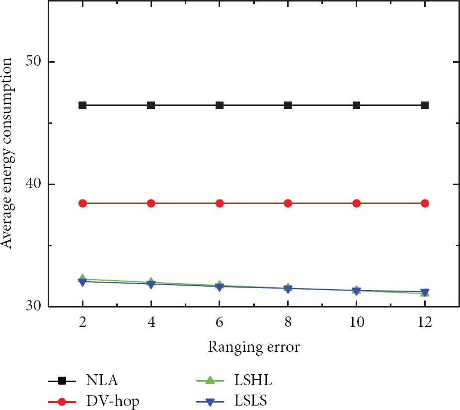
Average energy consumption with different ranging errors.

4.5. Impact of the Number of Anchor Nodes

In this part, we analyze the influence of the number of anchor nodes. In this set of simulations, we set trust threshold to be 0.95 and communication range to be 100 m. The number of anchor nodes changes from 80 to 140. Simulation results are shown as follows.

Figure 13 shows the relationship between localization coverage and the number of anchor nodes. For NLA and DV-hop algorithms, localization coverage changes slowly with the increase of the number of anchor nodes. Besides, the number of anchor nodes has a very small impact on the localization coverage for NLA and DV-hop algorithms. At the beginning, localization coverage of LSHL and LSLS algorithms increases with the increase in the number of anchor nodes. When the number of anchor nodes continues to increase, localization coverage will not change obviously, because with the increase in the number of anchor nodes in the network, more ordinary nodes can upgrade to be reference nodes to help another ordinary node with localization, which brings a larger localization coverage.

Figure 13

Localization coverage with varying number of anchor nodes.

We can observe from Figure 14 that localization errors of NLA and DV-hop algorithms decrease with the increase in number of anchor nodes, because the calculated one-hop distance can achieve higher accuracy with the increase in the number of anchor nodes, which contributes to the decrease in localization errors. For LSHL and LSLS algorithms, localization errors decrease slowly with the increase in the number of anchor nodes. With more anchor nodes deployed in the network, more ordinary nodes have opportunities to communicate with anchor nodes directly, which can improve the localization accuracy.

Figure 14

Localization error with varying number of anchor nodes.

Figure 15 depicts the influence of the number of anchor nodes on average energy consumption. For NLA and DV-hop algorithms, more message packages will be exchanged when the number of anchor nodes increases; that is why the average energy consumption increases with the increase in number of anchor nodes. For LSHL and LSLS algorithms, more ordinary nodes can be localized with the increase in the number of anchor nodes, which leads to the increase in total energy consumption.

Figure 15

Localization coverage with varying number of anchor nodes.

5. Conclusion

Localization is a fundamental and important task in UASNs. In this paper, we introduce four distributed localization algorithms for large-scale UASNs and compare the performance of them in terms of localization coverage, localization error, and average energy consumption. Simulations show that LSLS and LSHL algorithms can achieve higher localization coverage, lower localization error, and average energy consumption than DV-hop and NLA algorithms. The advantage of NLA and DV-hop algorithms is that they are range-free localization algorithms and do not need any extra hardware to realize localization. NLA and DV-hop algorithms can be used in situations where localization accuracy is not so emphasized. The NLA algorithm performs better than the DV-hop algorithm in the aspects of localization coverage and localization error. Besides, we analyze the impact of the ranging error and the number of anchor nodes on the performance of the algorithms. Simulations show that the localization coverage and localization accuracy can be improved with the increase in the number of anchor nodes, especially for LSHL and LSLS algorithms.

In the future, we will propose more effective localization algorithms based on the existing algorithms. Besides, localization in mobile UASNs will be investigated and studied.