Automatic Deduction Theorem of Overall Transfer Equation of Multibody System

Abstract

Transfer matrix method for multibody System (MSTMM) is a new multibody dynamics method developed in recent 20 years. It has been widely used in both science research and engineering for its special features as follows: without global dynamics equations of the system, high programming, low order of system matrix, and high computational speed. Based on MSTMM and its above features, a theorem to deduce automatically the overall transfer equations of multibody systems by handwriting or by computer is proposed in this paper. The theorem is effective for multibody systems with various topological structures, including chain systems, closed-loop systems, tree systems, general systems composed of one tree subsystem, and some closed-loop subsystems. This theorem makes it possible to program large scale software of multibody system dynamics with muchhigher programming, and much higher computational speed because of the above features of MSTMM. Formulations of the proposed method as well as two examples are given to verify this method.

1. Introduction

Lots of methods dealing with multibody system dynamics (MSD) have been studied by many authors since 1960s [1–18]. They are widely used in many engineering fields such as aeronautics, astronautics, spacecraft, vehicle, robot, precision machinery, and biomechanics. It is well known that almost all the previous ordinary methods for MSD have the same characteristics as follows: it is necessary and very complicated to develop the global dynamics equations of the system; the order of system matrix depends on the number of degrees of freedom of the system and hence it is rather high for complex multibody system.

To avoid establishing the global dynamics equations of the system, simplify the study procedure and especially keep high computational efficiency independent of the number of degree of freedom of system in studying MSD, new analytical method for MSD, namely, transfer matrix method for multibody system (MSTMM), is presented by Rui and his co-workers [19–21] and constantly developed in recent 20 years [22–25]. Nowadays, MSTMM is widely applied in science research and engineering [26–29] for the features of this method as follows: study MSD without global dynamics equations of the system, keep low order of the system matrix so very high computational speed, and avoid the difficulties in computation caused by high-order matrices and high programming. It has been proved by lots of theories and experiments that MSTMM is effective for linear time-invariant multibody systems [22], nonlinear time-variant multibody systems, multi-rigid-body systems [19, 21], multi-rigid-flexible-body systems [22–24], and controlled multibody systems [19, 29].

Generally speaking, various multibody systems may be considered as one of the following four cases in topology [24]: (1) chain system, (2) closed-loop system, (3) tree system, (4) general systems composed of one tree subsystem, and some closed-loop subsystems. A chain system can be considered as a special example of a tree system at the case with only two boundary ends. By “cutting” at one connection point of a system, a closed-loop system can be considered as a chain system, and a general system composed of one tree subsystem and some closed-loop subsystems can be dealt with a tree system [24]. Based on MSTMM and its above features, a theorem to deduce automatically the overall transfer equations of various multibody systems mentioned above by handwriting and by computer is proposed in this paper.

2. General Theorems and Steps of MSTMM

2.1. Basic Idea of MSTMM

The basic idea of MSTMM [19] is to break up a multibody system into the elements containing bodies (including rigid bodies, flexible bodies, lumped masses, etc.) and hinges (including joints, ball-and-sockets, pins, springs, rotary springs, dampers and rotary dampers, etc.) whose dynamics properties can be readily expressed in matrix forms. These matrices of elements are considered as building blocks that provide the dynamics properties of the entire system when assembling them together according to the topology of the system. Particularly, the positions of bodies and hinges are considered equivalent in transfer equations and transfer matrices, which is totally different from ordinary methods for MSD [1–18] and results in the very low order of system matrix and very high computational speed in MSTMM.

2.2. State Vector, Transfer Equation, and Transfer Matrix of Element

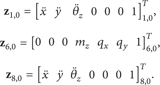
The same coordinate systems and sign conventions as are described in [19, 21, 30] will be used. The state vector of the connection point between any rigid body and hinge moving in space is defined as

$\mathbf{z}={\left[\begin{array}{ccccccccccccc}\ddot{x}& \ddot{y}& \ddot{z}& {\ddot{\theta }}_x& {\ddot{\theta }}_y& {\ddot{\theta }}_z& m_x& m_y& m_z& q_x& q_y& q_z& 1\end{array}\right]}^T,$

(1)

or

$\mathbf{z}={\left[\begin{array}{ccccc}{\ddot{\mathbf{r}}}^T& {\ddot{\mathit{\theta }}}^T& {\mathbf{m}}^T& {\mathbf{q}}^T& 1\end{array}\right]}^T,$

(2)

where

$\begin{array}{c}\ddot{\mathit{r}}=\left[\begin{array}{c}\ddot{x}\\ \ddot{y}\\ \ddot{z}\end{array}\right],\hspace{1em}\hspace{1em}\ddot{\mathit{\theta }}=\left[\begin{array}{c}{\ddot{\theta }}_x\\ {\ddot{\theta }}_y\\ {\ddot{\theta }}_z\end{array}\right],\\ \mathit{m}=\left[\begin{array}{c}{m}_x\\ m_y\\ m_z\end{array}\right],\hspace{1em}\hspace{1em}\mathit{q}=\left[\begin{array}{c}{q}_x\\ q_y\\ q_z\end{array}\right].\end{array}$

(3)

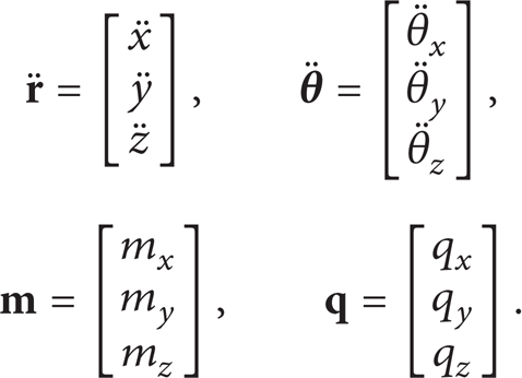
The state vector of connection point between flexible body and hinge moving in space is defined as

$\begin{array}{c}\mathbf{z}=[\ddot{x},\ddot{y},\ddot{z},{\ddot{\theta }}_x,{\ddot{\theta }}_y,{\ddot{\theta }}_z,m_x,m_y,m_z,\\ {q_x,q_y,q_z,{\ddot{q}}^{\mathrm{1}},{\ddot{q}}^{\mathrm{2}},\dots ,{\ddot{q}}^n,\mathrm{1}]}^T,\end{array}$

(4)

where $\ddot{x}$ , $\ddot{y}$ , and $\ddot{z}$ are the accelerations of the connection point with respect to the global inertial coordinate system oxyz; ${\ddot{\theta }}_x$ , ${\ddot{\theta }}_y$ , and ${\ddot{\theta }}_z$ are the second time derivatives of the orientation angles of the body using space-three-angles 1–2–3 θ _x , θ _y , and θ _z defined in [18]; m_x, m_y, m_z, q_x, q_y, and q_z are the corresponding internal torques and internal forces in the same reference system, respectively; ${\ddot{q}}^{\mathrm{1}},{\ddot{q}}^{\mathrm{2}},\dots ,{\ddot{q}}^n$ are the second time derivatives of the generalized coordinates describing the deformation of flexible bodies using modal method; the superscript n is the highest order of the modal considered, $\ddot{\mathit{r}}$ , $\ddot{\mathit{\theta }}$ , m , and q are the column matrices of accelerations, second time derivatives of the space-three angles, internal torques, and internal forces in oxyz, respectively.

For body and hinge elements moving in a plane, a similar definition of the state vector can be introduced, which is a special example of spatial motion.

The transfer equations of the jth element can be obtained easily by rewriting its dynamics equations as follows [19, 21, 30]

${\mathbf{z}}_{j,j+\mathrm{1}}={\mathit{U}}_j\left(t_i\right){\mathbf{z}}_{j,j-\mathrm{1}},$

(5)

where U _j (t _i ) is the transfer matrix of the jth element, which expresses the relationship between the state vectors of its output end z_{j,j + 1} and input end z_j,j–1 and is already known at time instant t_i.

It should be pointed out that there are general linear relations among accelerations, angular accelerations, forces, and torques of any mechanics system in an inertial coordinate system oxyz, according to Newton motion law and Euler theorem of moment of momentum. It is to say that there are strict linear relations between the state vectors of output end and input end of any element and among all state vectors of a multibody system. Thus, the transfer equation (5) is a general equation and effective for any mechanics element in the inertial coordinate system.

2.3. Overall Transfer Equation and Overall Transfer Matrix of the System

The overall transfer equations of a chain system can be deduced automatically as [19, 24]

${\mathbf{z}}_{\mathrm{1,0}}={\mathit{U}}_{n-\mathrm{1}}{\mathbf{z}}_{n,\mathrm{0}},$

(6)

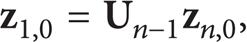
where the overall transfer matrix of the system is

${\mathit{U}}_{n-\mathrm{1}}={\mathit{U}}_{\mathrm{1}}{\mathit{U}}_{\mathrm{2}}{\mathit{U}}_{\mathrm{3}}\cdots {\mathit{U}}_n.$

(7)

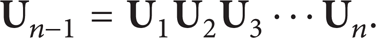
From equations (6) and (7), the features of the overall transfer equation for a chain system can be clearly seen; overall transfer matrix of a chain system can be deduced automatically by successive premultiplication of transfer matrices of every element of the system along the transfer path from the one end to another end.

2.4. Solutions of the System Motion

Applying the boundary conditions of the system, z_1,0 and z_n,0, to the overall system transfer equation (6), the unknown state variables in the boundary state vectors can be computed. Then, the state vectors of each element at time t_i can be computed by the repeated use of corresponding transfer equations of element (5). Then, using the computed values of the last step as the initial conditions, the entire procedure can be repeated from time t_{i + 1} until the time required for complete analysis. It can be seen clearly from equations (5)–(7) that MSTMM belongs to one of strict analytical methods in principle.

3. Topology Figure of a Multibody System and Sign Conventions

3.1. Topology Figure of a Multibody System

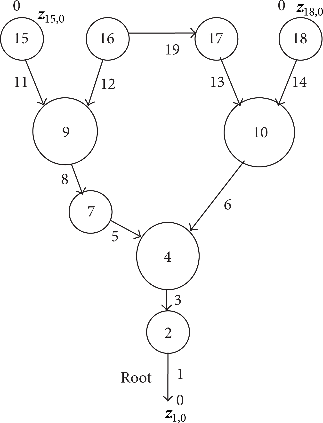
A dynamics model of any complex multibody system can be constructed with dynamics elements including bodies and hinges. In order to describe the transfer relationship among the state vectors of elements and the transfer directions in a system, the topology Figure of the model will be very useful for deduction of overall transfer equation in MSTMM. And the topology figure of the dynamics model of a system, for example, a tree multibody system, as shown in Figure 1, can be got very easily and directly from its dynamics model if using the following sign conventions.

Figure 1:

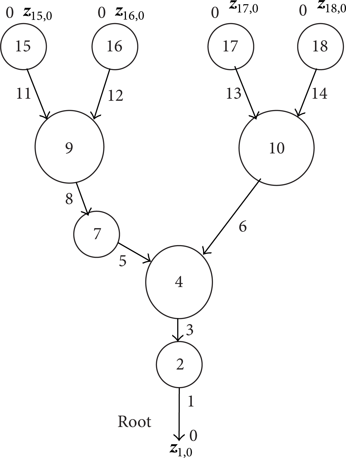
Topology figure of a dynamics model of tree multibody system.

3.2. The Sign Conventions

Besides the sign conventions introduced in [19, 21], the sign conventions as follows are used in the paper.

1. A circle ○ denotes a body element and the number inside this circle is the sequence number of the body element.

2. An arrow → denotes a hinge element and the transfer direction of state vectors; the number beside the arrow is the sequence number of the hinge element.

3. Each body element is dealt with single output end and single input end if the body has two connection ends with other elements; otherwise, it is dealt with single output end and multiple input ends if the body has more two connection ends.

4. For a nonboundary end, the first and second subscripts, i and j (i,j≠0), in a state vector z_i,j of the end denote the sequence numbers of the adjacent body element and hinge element, respectively. For a boundary end, the second subscript j = 0 in the state vector z_i,j that is, the second subscript 0 means boundary end; then the first subscript i in the state vector z_i,0 of the boundary end stands for the sequence number of the element involved.

5. In a multibody system, only one boundary end is considered as the root; the state vector of root is noted as z_i,0, where i is the sequence number of the root element; all of other boundary ends are considered as the tips; the state vectors of tips are denoted as z_j,0, where j is the sequence number of the tip element. The transfer directions of a system are always from its tips to the root.

6. The subscript i in transfer matrix U i denotes the sequence number of element i. The subscript (i-k) in the transfer matrix U _i-k and the partitioned matrix u _i-k means from element i to element k. U _i-k and u _i-k mean the successive premultiplication of the transfer matrices of all elements in the transfer path from the element i to element k of the system.

4. Automatic Deduction of Overall Transfer Equations of System

4.1. Automatic Deduction of the Overall Transfer Equation of a Chain System

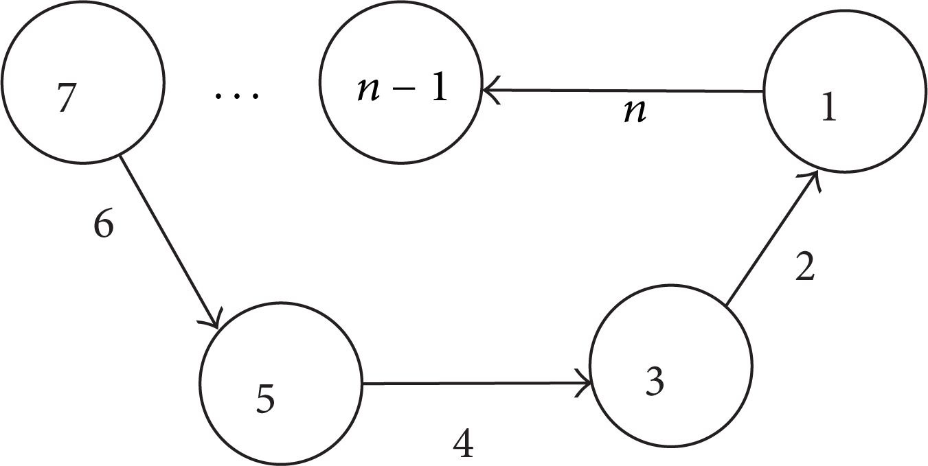
The topology Figure of any chain system is shown in Figure 2.

Figure 2:

Topology figure of a chain system.

It is clear that we can rewrite the overall transfer equation (6) of the chain system as

${\mathbf{U}}_{\text{all}}{\left[\begin{array}{cc}{\mathbf{z}}_{\mathrm{1,0}}^T& {\mathbf{z}}_{n,\mathrm{0}}^T\end{array}\right]}^T=\mathrm{0},\hspace{1em}{\mathbf{U}}_{\text{all}}=\left[\begin{array}{cc}-\mathbf{I}& {\mathbf{U}}_{n-\mathrm{1}}\end{array}\right].$

(8)

From equations (6) or (7), it can be seen clearly that the overall transfer matrix of any chain system U_all can be deduced automatically by handwriting and by computer. In the overall transfer matrix, the coefficient matrix of the state vector of root is a minus unit matrix I, while the coefficient matrix of the state vector of tip U_n–1 is the successive premultiplication of the transfer matrices of all elements in the transfer path from this tip to the root as shown in equation (7).

The highest order of the overall transfer matrix is 13 for spatial chain multi-rigid-body system or (13 + n) for chain multi-rigid-flexible-body system, where n is the highest order of the modal considered.

4.2. Automatic Deduction of the Overall Transfer Equations of a Closed-Loop System

For any closed-loop system, whose topology Figure is shown in Figure 3, after “cutting” at the junction of any two adjacent elements such as body 1 and hinge n as shown in Figure 4, consider the couple of “cutting point” as the “boundary ends” with the same state vectors noted as z_n,0 and z_1,0. Then the original closed-loop system becomes a chain system with the same “boundary ends” state vectors, z_n,0 and z_1,0, as shown in Figure 4.

Figure 3:

Topology figure of a closed-loop system.

Figure 4:

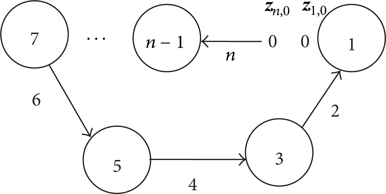
Topology figure of a closed-loop system after “cutting” the hinge n.

Thus, the transfer equation of the closed-loop system can be deduced automatically as is achieved for the chain system

${\mathbf{z}}_{\mathrm{1,0}}={\mathbf{U}}_{n-\mathrm{1}}{\mathbf{z}}_{n,\mathrm{0}}$

(9)

according to the proposed sign conventions, where

${\mathbf{U}}_{n-\mathrm{1}}={\mathbf{U}}_{\mathrm{1}}{\mathbf{U}}_{\mathrm{2}}{\mathbf{U}}_{\mathrm{3}}\cdots {\mathbf{U}}_n.$

(10)

Attention should be paid that the state vectors of a couple of “cutting points” are the same, namely

${\mathbf{z}}_{n,\mathrm{0}}={\mathbf{z}}_{\mathrm{1,0}}.$

(11)

Then, the transfer equation (9) of the closed-loop system can be deduced automatically by handwriting and by computer

${\mathbf{U}}_{\text{all}}{\mathbf{z}}_{\mathrm{1,0}}=\mathrm{0},\hspace{1em}{\mathbf{U}}_{\text{all}}=\left(\mathbf{I}-{\mathbf{U}}_{n-\mathrm{1}}\right).$

(12)

4.3. Automatic Deduction of the Overall Transfer Equations of a Tree System

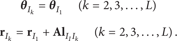
For each body element with more than two ends, as is mentioned in the convention, only one of the ends is considered as output end and all the other ends are input ends. Moreover, its transfer equations should cover the geometrical relationship between its first input end and output end and describe the mechanical principle for the forces and moments acting on the element. Thus, it can be verified later that the transfer equations of a rigid body j with L input ends can be written in the following form

${\mathbf{z}}_{j,O}={\mathbf{U}}_j{\mathbf{z}}_{j,I_{\mathrm{1}}}+{\mathbf{U}}_{j,I_{\mathrm{2}}}{\mathbf{z}}_{j,I_{\mathrm{2}}}+\cdots +{\mathbf{U}}_{j,I_L}{\mathbf{z}}_{j,I_L},$

(13)

where the subscript j is the sequence number of the body; O and I₁,I₂,I₃⋯I _L denote the output end and input ends respectively, and the first input end I1 is considered as the dominant input end; z_j,O and z_{j,I k} (k = 2, 3, 4,…, L) are the state vectors of the output end and the kth input end of the body element respectively; Uj is just the transfer matrix of element j when point I1 and point O are considered as the only input end and output end of this element; U_{j,I k} is the corresponding extraction matrix that extracts the force variables (including internal force and internal moment) from the state vector when it premultiplies z_{j,I k} , acted on the same point.

However, in equation(13), the number of unknown variables is more than that of algebraic equations. Therefore, geometrical equations of the body, which describes the geometrical relationship between the first input end and kth (k = 2, 3, 4,…, L) input end of the body, should be introduced for body elements with single output end and multiple input ends. It is verified later that the geometrical equation can be written in the form of

${\mathbf{H}}_j{\mathbf{z}}_{j,I_{\mathrm{1}}}={\mathbf{H}}_{j,I_k}{\mathbf{z}}_{j,I_k}\hspace{1em}\left(k=\mathrm{2,3},\mathrm{4},\dots ,L\right),$

(14)

where Hj is a constant matrix extracting displacement variables (including position coordinates and orientation angles) from a state vector when premultiplying z_j,I1 H_{j,I k} is related to the relative position between the first input end and kth input end of body. The number of the geometrical equations is (L–1).

A spatial motion rigid body with more than two ends is shown in Figure 5; the concrete form of the transfer equations and geometrical equations of body element will be exhibited.

Figure 5:

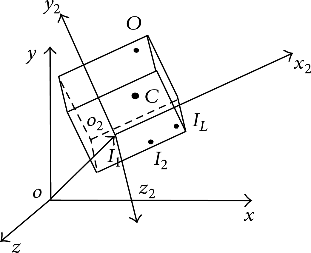
A spatial motion rigid body with more than two ends.

The state vectors of inboard ends and outboard ends of the rigid body, as defined in Section 2.2, are

$\begin{array}{c}{\mathbf{z}}_{I_k}={\left[\ddot{x},\ddot{y},\ddot{z},{\ddot{\theta }}_x,{\ddot{\theta }}_y,{\ddot{\theta }}_z,m_x,m_y,m_z,q_x,q_y,q_z,\mathrm{1}\right]}_{I_k}^T\\ \hspace{1em}\hspace{1em}\hspace{1em}\hspace{1em}\hspace{1em}\hspace{1em}\hspace{1em}\hspace{1em}\hspace{1em}\hspace{1em}\hspace{1em}\hspace{1em}\hspace{1em}\hspace{1em}\left(k=\mathrm{1,2},\dots ,L\right)\\ {\mathbf{z}}_O={\left[\ddot{x},\ddot{y},\ddot{z},{\ddot{\theta }}_x,{\ddot{\theta }}_y,{\ddot{\theta }}_z,m_x,m_y,m_z,q_x,q_y,q_z,\mathrm{1}\right]}_O^T.\end{array}$

(15)

As shown in Figure 5, I _k (k = 1, 2,…, L), O, and C denote the inboard ends, outboard end, and mass center of the rigid body, respectively; the coordinate system with subscript 2 denotes the body-fixed coordinate system whose initial point o2 is on the first inboard end I1 of the rigid body. According to the properties of a rigid body, the geometrical relationship between the first inboard end and the outboard end of the rigid body can be obtained as

$\begin{array}{c}{\mathbf{\theta }}_O={\mathbf{\theta }}_{I_{\mathrm{1}}},\\ {\mathbf{r}}_O={\mathbf{r}}_{I_{\mathrm{1}}}+\mathbf{A}{\mathbf{l}}_{I_{I}O},\end{array}$

(16)

where θ _{I 1} and θO are the column matrices of the orientation coordinates of the first inboard end I1 and the outboard end O; rO and l _{I I O} are the column matrices of the position coordinates of point O with respect to the global inertial coordinate system oxyz and the body-fixed coordinate system o₂x₂y₂z₂ respectively; A is the direction cosine matrix that defines the orientation of the body-fixed coordinate system o₂x₂y₂z₂ in the global inertial coordinate system oxyz.

Similarly, the geometrical equations between the first inboard end I1 and the other inboard ends I _k (k = 1, 2,…, L) can be obtained easily

$\begin{array}{c}{\mathbf{\theta }}_{I_k}={\mathbf{\theta }}_{I_{\mathrm{1}}}\hspace{1em}\left(k=\mathrm{2,3},\dots ,L\right)\\ {\mathbf{r}}_{I_k}={\mathbf{r}}_{I_{\mathrm{1}}}+\mathbf{A}{\mathbf{l}}_{I_I{I}_k}\hspace{1em}\left(k=\mathrm{2,3},\dots ,L\right).\end{array}$

(17)

Using Newton's laws of motion and considering the sign conventions, the dynamics equations of the rigid body can be obtained in the global inertial reference frame as [30]

$\begin{array}{c}m{\ddot{\mathbf{r}}}_C={\displaystyle \sum }_{k=\mathrm{1}}^L{\mathbf{q}}_{I_k}-{\mathbf{q}}_O+{\mathbf{f}}_C,\\ {\dot{\mathbf{G}}}_{I_{\mathrm{1}}}=-{\displaystyle \sum }_{k=\mathrm{1}}^L{\mathbf{m}}_{I_k}+{\displaystyle \sum }_{k=\mathrm{2}}^L{\tilde{\mathbf{r}}}_{I_{\mathrm{1}}{I}_k}{\mathbf{q}}_{I_k}+{\mathbf{m}}_O-{\tilde{\mathbf{r}}}_{I_{\mathrm{1}}O}{\mathbf{q}}_O-\mathbf{m}{\tilde{\mathbf{r}}}_{I_{\mathrm{1}}C}{\ddot{\mathbf{r}}}_{I_{\mathrm{1}}}+{\mathbf{m}}_C+{\tilde{\mathbf{r}}}_{I_{\mathrm{1}}C}{\mathbf{f}}_C,\end{array}$

(18)

where m and ${\ddot{\mathbf{r}}}_C$ are the mass and the column matrix of mass center acceleration of the rigid body respectively; q _{I k} (k = 1,2,…, L) and qO are the column matrices of internal forces acting on the point I _k (k = 1,2,…, L) and O, respectively; fC and mC are the column matrices of external force and the external torque acting on the mass center of the rigid body; G _{I 1} is the column matrix of relative moment of momentum with respect to the first input end I1 of the body element; m _{I k} (k = 1,2,…, L) and mO are the column matrices of internal torques acting on points I _k (k = 1,2,…, L) and O, respectively; r _{I 1 P} represents the column matrix of position vectors from I1 to point P with respect to the inertial coordinate system, where P represents I _k (k = 2,3,…, L), C, or O.

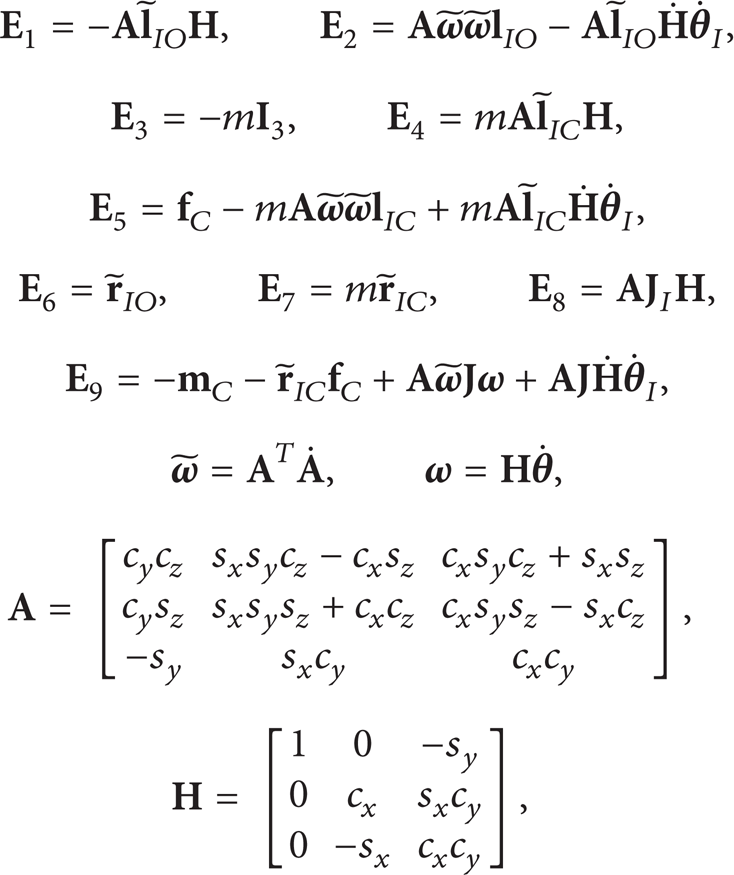
By equations (16), (18), and rewriting them in the form of equation (13), transfer matrices can be obtained as

$\begin{array}{c}{\mathbf{U}}_j=\left[\begin{array}{ccccc}{\mathbf{I}}_{\mathrm{3}}& {\mathbf{E}}_{\mathrm{1}}& {\mathbf{O}}_{\mathrm{3}\times \mathrm{3}}& {\mathbf{O}}_{\mathrm{3}\times \mathrm{3}}& {\mathbf{E}}_{\mathrm{2}}\\ {\mathbf{O}}_{\mathrm{3}\times \mathrm{3}}& {\mathbf{I}}_{\mathrm{3}}& {\mathbf{O}}_{\mathrm{3}\times \mathrm{3}}& {\mathbf{O}}_{\mathrm{3}\times \mathrm{3}}& {\mathbf{O}}_{\mathrm{3}\times \mathrm{1}}\\ {\mathbf{E}}_{\mathrm{6}}{\mathbf{E}}_{\mathrm{3}}+{\mathbf{E}}_{\mathrm{7}}& {\mathbf{E}}_{\mathrm{6}}{\mathbf{E}}_{\mathrm{4}}+{\mathbf{E}}_{\mathrm{8}}& {\mathbf{I}}_{\mathrm{3}}& {\mathbf{E}}_{\mathrm{6}}& {\mathbf{E}}_{\mathrm{6}}{\mathbf{E}}_{\mathrm{5}}+{\mathbf{E}}_{\mathrm{9}}\\ {\mathbf{E}}_{\mathrm{3}}& {\mathbf{E}}_{\mathrm{4}}& {\mathbf{O}}_{\mathrm{3}\times \mathrm{3}}& {\mathbf{I}}_{\mathrm{3}}& {\mathbf{E}}_{\mathrm{5}}\\ {\mathbf{O}}_{\mathrm{1}\times \mathrm{3}}& {\mathbf{O}}_{\mathrm{1}\times \mathrm{3}}& {\mathbf{O}}_{\mathrm{1}\times \mathrm{3}}& {\mathbf{O}}_{\mathrm{1}\times \mathrm{3}}& \mathrm{1}\end{array}\right],\end{array}$

(19)

where lAB is the column matrix of the position vector from point A to point B in the body-fixed coordinate whose original point is the first input end I1; ${\tilde{\mathbf{l}}}_{AB}$ is the cross product matrix of lAB. The meanings of other signs are the same with those in [19, 30].

By geometrical equations (17) and rewriting them in the form of equation (14), the concrete form of matrices Hj and H_{j,I k} can be acquired as

$\begin{array}{c}{\mathbf{U}}_{j,I_k}=\left[\begin{array}{ccccc}{\mathbf{O}}_{\mathrm{3}\times \mathrm{3}}& {\mathbf{O}}_{\mathrm{3}\times \mathrm{3}}& {\mathbf{O}}_{\mathrm{3}\times \mathrm{3}}& {\mathbf{O}}_{\mathrm{3}\times \mathrm{3}}& {\mathbf{O}}_{\mathrm{3}\times \mathrm{1}}\\ {\mathbf{O}}_{\mathrm{3}\times \mathrm{3}}& {\mathbf{O}}_{\mathrm{3}\times \mathrm{3}}& {\mathbf{O}}_{\mathrm{3}\times \mathrm{3}}& {\mathbf{O}}_{\mathrm{3}\times \mathrm{3}}& {\mathbf{O}}_{\mathrm{3}\times \mathrm{1}}\\ {\mathbf{O}}_{\mathrm{3}\times \mathrm{3}}& {\mathbf{O}}_{\mathrm{3}\times \mathrm{3}}& {\mathbf{I}}_{\mathrm{3}}& {\tilde{\mathbf{r}}}_{I_{\mathrm{1}}{I}_k}& {\mathbf{O}}_{\mathrm{3}\times \mathrm{1}}\\ {\mathbf{O}}_{\mathrm{3}\times \mathrm{3}}& {\mathbf{O}}_{\mathrm{3}\times \mathrm{3}}& {\mathbf{O}}_{\mathrm{3}\times \mathrm{3}}& {\mathbf{I}}_{\mathrm{3}}& {\mathbf{O}}_{\mathrm{3}\times \mathrm{1}}\\ {\mathbf{O}}_{\mathrm{1}\times \mathrm{3}}& {\mathbf{O}}_{\mathrm{1}\times \mathrm{3}}& {\mathbf{O}}_{\mathrm{1}\times \mathrm{3}}& {\mathbf{O}}_{\mathrm{1}\times \mathrm{3}}& \mathrm{1}\end{array}\right]\\ \phantom{\text{hhhhhhhhhhhhhhh}}\phantom{\text{hhhh}}(k=\mathrm{2,3},\mathrm{4},\dots ,L),\end{array}$

(20)

It can be clearly seen from equation (19) that the matrix is exactly the same with the transfer matrix of rigid body with single input end and single output end, which in fact can be regarded as a special case of rigid body with more than two ends (multiple input ends and single output end).

Based on the transfer equations and geometrical equations of elements, it is then easy to get the overall transfer equation of the system automatically.

According to the topology Figure of the system shown in Figure 1, the relations among the state vectors and transfer equations of elements can been described more intuitively and directly using topology described by state vectors and transfer equations as shown in Figure 6.

Figure 6:

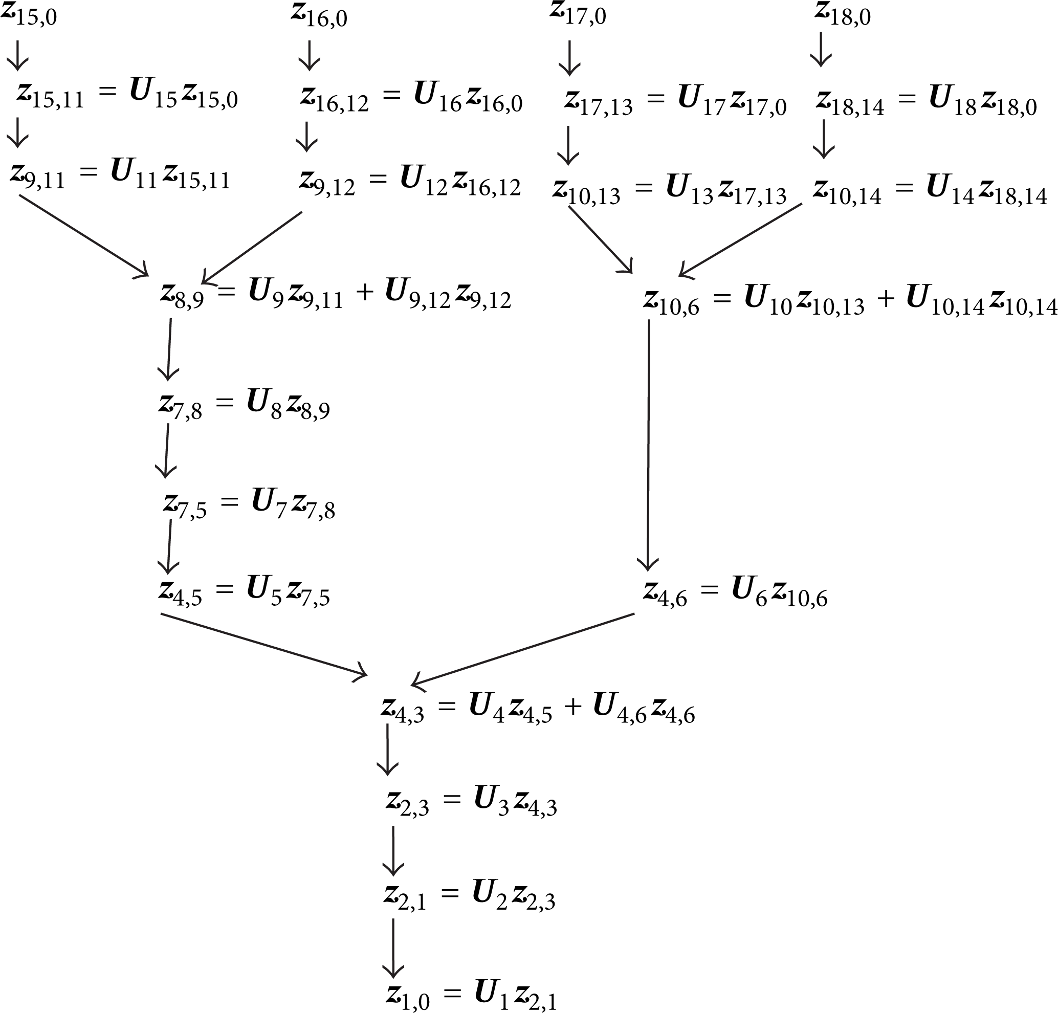
System topology described by state vectors and transfer equations.

Then the main transfer equations of the system in Figure 6 can be easily deduced, that is,

$\begin{array}{c}{\mathbf{E}}_{\mathrm{1}}=-\mathbf{A}{\tilde{\mathbf{l}}}_{IO}\mathbf{H},\hspace{1em}\hspace{1em}{\mathbf{E}}_{\mathrm{2}}=\mathbf{A}\tilde{\mathbf{\omega }}\tilde{\mathbf{\omega }}{\mathbf{l}}_{IO}-\mathbf{A}{\tilde{\mathbf{l}}}_{IO}\dot{\mathbf{H}}{\dot{\mathbf{\theta }}}_I,\\ {\mathbf{E}}_3=-m{\mathit{I}}_3,\hspace{1em}\hspace{1em}{\mathbf{E}}_4=m\mathit{A}{\tilde{\mathbf{l}}}_{IC}\mathit{H},\\ {\mathbf{E}}_{\mathrm{5}}={\mathbf{f}}_C-m\mathbf{A}\tilde{\mathbf{\omega }}\tilde{\mathbf{\omega }}{\mathbf{l}}_{IC}+m\mathbf{A}{\tilde{\mathbf{l}}}_{IC}\dot{\mathbf{H}}{\dot{\mathbf{\theta }}}_I,\\ {\mathbf{E}}_{\mathrm{6}}={\tilde{\mathbf{r}}}_{IO},\hspace{1em}\hspace{1em}{\mathbf{E}}_{\mathrm{7}}=m{\tilde{\mathbf{r}}}_{IC},\hspace{1em}\hspace{1em}{\mathbf{E}}_{\mathrm{8}}=\mathbf{A}{\mathbf{J}}_I\mathbf{H}\mathbf{,}\\ {\mathbf{E}}_{\mathrm{9}}=-{\mathbf{m}}_C-{\tilde{\mathbf{r}}}_{IC}{\mathbf{f}}_C+\mathbf{A}\tilde{\mathbf{\omega }}\mathbf{J}\mathbf{\omega }+\mathbf{A}\mathbf{J}\dot{\mathbf{H}}{\dot{\mathbf{\theta }}}_I,\\ \tilde{\mathbf{\omega }}={\mathbf{A}}^T\dot{\mathbf{A}},\hspace{1em}\hspace{1em}\mathbf{\omega }=\mathbf{H}\dot{\mathbf{\theta }},\\ \mathbf{A}=\left[\begin{array}{ccc}{c}_y{c}_z& s_x{s}_y{c}_z-c_x{s}_z& c_x{s}_y{c}_z+s_x{s}_z\\ c_y{s}_z& s_x{s}_y{s}_z+c_x{c}_z& c_x{s}_y{s}_z-s_x{c}_z\\ -s_y& s_x{c}_y& c_x{c}_y\end{array}\right],\\ \mathbf{H}=\left[\begin{array}{ccc}\mathrm{1}& \mathrm{0}& -s_y\\ \mathrm{0}& c_x& s_x{c}_y\\ \mathrm{0}& -s_x& c_x{c}_y\end{array}\right],\end{array}$

(21)

where

$\begin{array}{c}{\mathbf{H}}_j=\left[\begin{array}{cc}{\mathbf{I}}_{\mathrm{6}}& {\mathbf{O}}_{\mathrm{6}\times \mathrm{7}}\end{array}\right]\\ {\mathbf{H}}_{j,I_k}=\left[\begin{array}{ccccc}{\mathbf{I}}_{\mathrm{3}}& \mathbf{A}{\tilde{\mathbf{l}}}_{I_{\mathrm{1}}{I}_k}\mathbf{H}& {\mathbf{O}}_{\mathrm{3}\times \mathrm{3}}& {\mathbf{O}}_{\mathrm{3}\times \mathrm{3}}& \mathbf{A}{\tilde{\mathbf{l}}}_{I_{\mathrm{1}}{I}_k}\dot{\mathbf{H}}\dot{\mathbf{\theta }}-\mathbf{A}\tilde{\mathbf{\omega }}\tilde{\mathbf{\omega }}{\mathbf{l}}_{I_{\mathrm{1}}{I}_k}\\ {\mathbf{O}}_{\mathrm{3}\times \mathrm{3}}& {\mathbf{I}}_{\mathrm{3}}& {\mathbf{O}}_{\mathrm{3}\times \mathrm{3}}& {\mathbf{O}}_{\mathrm{3}\times \mathrm{3}}& {\mathbf{O}}_{\mathrm{3}\times \mathrm{1}}\end{array}\right]\\ (k=\mathrm{2,3},\mathrm{4},\dots ,L).\end{array}$

(22)

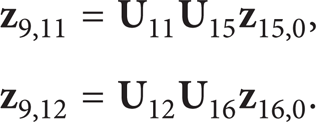
Further, the geometrical equation of the body element 9 is

$\begin{array}{c}{\mathbf{z}}_{\mathrm{1,0}}={\mathbf{U}}_{\mathrm{1}}{\mathbf{z}}_{\mathrm{2,1}}={\mathbf{U}}_{\mathrm{1}}{\mathbf{U}}_{\mathrm{2}}{\mathbf{U}}_{\mathrm{3}}{\mathbf{z}}_{\mathrm{4,3}}={\mathbf{U}}_{\mathrm{1}}{\mathbf{U}}_{\mathrm{2}}{\mathbf{U}}_{\mathrm{3}}{\mathbf{U}}_{\mathrm{4}}{\mathbf{z}}_{\mathrm{4,5}}+{\mathbf{U}}_{\mathrm{1}}{\mathbf{U}}_{\mathrm{2}}{\mathbf{U}}_{\mathrm{3}}{\mathbf{U}}_{\mathrm{4,6}}{\mathbf{z}}_{\mathrm{4,6}}\\ \hspace{1em}\hspace{1em}\hspace{1em}={\mathbf{U}}_{\mathrm{1}}{\mathbf{U}}_{\mathrm{2}}{\mathbf{U}}_{\mathrm{3}}{\mathbf{U}}_{\mathrm{4}}{\mathbf{U}}_{\mathrm{5}}{\mathbf{U}}_{\mathrm{7}}{\mathbf{U}}_{\mathrm{8}}{\mathbf{z}}_{\mathrm{8,9}}+{\mathbf{U}}_{\mathrm{1}}{\mathbf{U}}_{\mathrm{2}}{\mathbf{U}}_{\mathrm{3}}{\mathbf{U}}_{\mathrm{4,6}}{\mathbf{U}}_{\mathrm{6}}{\mathbf{z}}_{\mathrm{10,6}}\\ \hspace{1em}\hspace{1em}\hspace{1em}={\mathbf{U}}_{\mathrm{1}}{\mathbf{U}}_{\mathrm{2}}{\mathbf{U}}_{\mathrm{3}}{\mathbf{U}}_{\mathrm{4}}{\mathbf{U}}_{\mathrm{5}}{\mathbf{U}}_{\mathrm{7}}{\mathbf{U}}_{\mathrm{8}}{\mathbf{U}}_{\mathrm{9}}{\mathbf{z}}_{\mathrm{9,11}}+{\mathbf{U}}_{\mathrm{1}}{\mathbf{U}}_{\mathrm{2}}{\mathbf{U}}_{\mathrm{3}}{\mathbf{U}}_{\mathrm{4}}{\mathbf{U}}_{\mathrm{5}}{\mathbf{U}}_{\mathrm{7}}{\mathbf{U}}_{\mathrm{8}}{\mathbf{U}}_{\mathrm{9,12}}{\mathbf{z}}_{\mathrm{9,12}}+{\mathbf{U}}_{\mathrm{1}}{\mathbf{U}}_{\mathrm{2}}{\mathbf{U}}_{\mathrm{3}}{\mathbf{U}}_{\mathrm{4,6}}{\mathbf{U}}_{\mathrm{6}}{\mathbf{U}}_{\mathrm{10}}{\mathbf{z}}_{\mathrm{10,13}}+{\mathbf{U}}_{\mathrm{1}}{\mathbf{U}}_{\mathrm{2}}{\mathbf{U}}_{\mathrm{3}}{\mathbf{U}}_{\mathrm{4,6}}{\mathbf{U}}_{\mathrm{6}}{\mathbf{U}}_{\mathrm{10,14}}{\mathbf{z}}_{\mathrm{10,14}}\\ \hspace{1em}\hspace{1em}\hspace{1em}={\mathbf{T}}_{\mathrm{15}-\mathrm{1}}{\mathbf{z}}_{\mathrm{15,0}}+{\mathbf{T}}_{\mathrm{16}-\mathrm{1}}{\mathbf{z}}_{\mathrm{16,0}}+{\mathbf{T}}_{\mathrm{17}-\mathrm{1}}{\mathbf{z}}_{\mathrm{17,0}}+{\mathbf{T}}_{\mathrm{18}-\mathrm{1}}{\mathbf{z}}_{\mathrm{18,0}},\end{array}$

(23)

Applying system topology described by state vectors and transfer equations in Figure 6, the state vectors z_9,11 and z_9,12 can be expressed using state vectors of system boundaries as

$\begin{array}{c}{\mathbf{T}}_{\mathrm{15}-\mathrm{1}}={\mathbf{U}}_{\mathrm{1}}{\mathbf{U}}_{\mathrm{2}}{\mathbf{U}}_{\mathrm{3}}{\mathbf{U}}_{\mathrm{4}}{\mathbf{U}}_{\mathrm{5}}{\mathbf{U}}_{\mathrm{7}}{\mathbf{U}}_{\mathrm{8}}{\mathbf{U}}_{\mathrm{9}}{\mathbf{U}}_{\mathrm{11}}{\mathbf{U}}_{\mathrm{15}},\\ {\mathbf{T}}_{\mathrm{16}-\mathrm{1}}={\mathbf{U}}_{\mathrm{1}}{\mathbf{U}}_{\mathrm{2}}{\mathbf{U}}_{\mathrm{3}}{\mathbf{U}}_{\mathrm{4}}{\mathbf{U}}_{\mathrm{5}}{\mathbf{U}}_{\mathrm{7}}{\mathbf{U}}_{\mathrm{8}}{\mathbf{U}}_{\mathrm{9,12}}{\mathbf{U}}_{\mathrm{12}}{\mathbf{U}}_{\mathrm{16}},\\ {\mathbf{T}}_{\mathrm{17}-\mathrm{1}}={\mathbf{U}}_{\mathrm{1}}{\mathbf{U}}_{\mathrm{2}}{\mathbf{U}}_{\mathrm{3}}{\mathbf{U}}_{\mathrm{4,6}}{\mathbf{U}}_{\mathrm{6}}{\mathbf{U}}_{\mathrm{10}}{\mathbf{U}}_{\mathrm{13}}{\mathbf{U}}_{\mathrm{17}},\\ {\mathbf{T}}_{\mathrm{18}-\mathrm{1}}={\mathbf{U}}_{\mathrm{1}}{\mathbf{U}}_{\mathrm{2}}{\mathbf{U}}_{\mathrm{3}}{\mathbf{U}}_{\mathrm{4,6}}{\mathbf{U}}_{\mathrm{6}}{\mathbf{U}}_{\mathrm{10,14}}{\mathbf{U}}_{\mathrm{14}}{\mathbf{U}}_{\mathrm{18}}.\end{array}$

(24)

Substituting equation (26) into equation (25), one obtains

${\mathbf{H}}_{\mathrm{9}}{\mathbf{z}}_{\mathrm{9,11}}={\mathbf{H}}_{\mathrm{9,12}}{\mathbf{z}}_{\mathrm{9,12}}.$

(25)

which can be written as

$\begin{array}{c}{\mathbf{z}}_{\mathrm{9,11}}={\mathbf{U}}_{\mathrm{11}}{\mathbf{U}}_{\mathrm{15}}{\mathbf{z}}_{\mathrm{15,0}},\\ {\mathbf{z}}_{\mathrm{9,12}}={\mathbf{U}}_{\mathrm{12}}{\mathbf{U}}_{\mathrm{16}}{\mathbf{z}}_{\mathrm{16,0}}.\end{array}$

(26)

where

$-{\mathbf{H}}_{\mathrm{9}}{\mathbf{U}}_{\mathrm{11}}{\mathbf{U}}_{\mathrm{15}}{\mathbf{z}}_{\mathrm{15,0}}+{\mathbf{H}}_{\mathrm{9,12}}{\mathbf{U}}_{\mathrm{12}}{\mathbf{U}}_{\mathrm{16}}{\mathbf{z}}_{\mathrm{16,0}}=\mathbf{0}$

(27)

Similarly, the geometrical equations corresponding to body elements 10 and 4 can be deduced as

${\mathbf{G}}_{\mathrm{15}-\mathrm{9}}{\mathbf{z}}_{\mathrm{15,0}}+{\mathbf{G}}_{\mathrm{16}-\mathrm{9}}{\mathbf{z}}_{\mathrm{16,0}}=\mathbf{0}\mathbf{,}$

(28)

where

$\begin{array}{c}{\mathbf{G}}_{\mathrm{15}-\mathrm{9}}=-{\mathbf{H}}_{\mathrm{9}}{\mathbf{U}}_{\mathrm{11}}{\mathbf{U}}_{\mathrm{15}},\\ {\mathbf{G}}_{\mathrm{16}-\mathrm{9}}={\mathbf{H}}_{\mathrm{9,12}}{\mathbf{U}}_{\mathrm{12}}{\mathbf{U}}_{\mathrm{16}}.\end{array}$

(29)

The overall transfer equation of the system can be obtained by combining the main transfer equation (23) and all the geometrical equations (28) and (30) of the system:

$\begin{array}{c}{\mathbf{G}}_{\mathrm{17}-\mathrm{10}}{\mathbf{z}}_{\mathrm{17,0}}+{\mathbf{G}}_{\mathrm{18}-\mathrm{10}}{\mathbf{z}}_{\mathrm{18,0}}=\mathbf{0}\mathbf{,}\\ {\mathbf{G}}_{\mathrm{15}-\mathrm{4}}{\mathbf{z}}_{\mathrm{15,0}}+{\mathbf{G}}_{\mathrm{16}-\mathrm{4}}{\mathbf{z}}_{\mathrm{16,0}}+{\mathbf{G}}_{\mathrm{17}-\mathrm{4}}{\mathbf{z}}_{\mathrm{17,0}}+{\mathbf{G}}_{\mathrm{18}-\mathrm{4}}{\mathbf{z}}_{\mathrm{18,0}}=\mathbf{0}\mathbf{,}\end{array}$

(30)

where

$\begin{array}{c}{\mathbf{G}}_{\mathrm{17}-\mathrm{10}}=-{\mathbf{H}}_{\mathrm{10}}{\mathbf{U}}_{\mathrm{13}}{\mathbf{U}}_{\mathrm{17}},\\ {\mathbf{G}}_{\mathrm{18}-\mathrm{10}}={\mathbf{H}}_{\mathrm{10,14}}{\mathbf{U}}_{\mathrm{14}}{\mathbf{U}}_{\mathrm{18}},\\ {\mathbf{G}}_{\mathrm{15}-\mathrm{4}}=-{\mathbf{H}}_{\mathrm{4}}{\mathbf{U}}_{\mathrm{5}}{\mathbf{U}}_{\mathrm{7}}{\mathbf{U}}_{\mathrm{8}}{\mathbf{U}}_{\mathrm{9}}{\mathbf{U}}_{\mathrm{11}}{\mathbf{U}}_{\mathrm{15}},\\ {\mathbf{G}}_{\mathrm{16}-\mathrm{4}}=-{\mathbf{H}}_{\mathrm{4}}{\mathbf{U}}_{\mathrm{5}}{\mathbf{U}}_{\mathrm{7}}{\mathbf{U}}_{\mathrm{8}}{\mathbf{U}}_{\mathrm{9,12}}{\mathbf{U}}_{\mathrm{12}}{\mathbf{U}}_{\mathrm{16}},\\ {\mathbf{G}}_{\mathrm{17}-\mathrm{4}}={\mathbf{H}}_{\mathrm{4,6}}{\mathbf{U}}_{\mathrm{6}}{\mathbf{U}}_{\mathrm{10}}{\mathbf{U}}_{\mathrm{13}}{\mathbf{U}}_{\mathrm{17}},\\ {\mathbf{G}}_{\mathrm{18}-\mathrm{4}}={\mathbf{H}}_{\mathrm{4,6}}{\mathbf{U}}_{\mathrm{6}}{\mathbf{U}}_{\mathrm{10,14}}{\mathbf{U}}_{\mathrm{14}}{\mathbf{U}}_{\mathrm{18}}.\end{array}$

(31)

According to the sign conventions and equations (32) and (33), it can be seen clearly that the overall transfer equation of the tree system, such as Figure 1, can be deduced automatically by handwriting and by computer. For more details, see Section 5 please.

As a short conclusion, in the overall transfer equation, z_all consists of all the state vectors at the boundary ends of system. Besides the main transfer equation, there exists a geometrical equation at multiple input body elements that finally leads to a branch in a tree system. Moreover, the number of geometrical equations in the overall transfer equation of a system is equal to the number of tips of a tree minus one. For the system shown in Figure 1, the number of the tips is 4; thus the number of geometric equations of the system is 3.

It can be seen clearly that overall transfer equation (8) of a chain system is a special example of overall transfer equations (32) and (33) at the case of the tree system with only two boundary ends.

4.4. Automatic Deduction of the Overall Transfer Equations of a General System

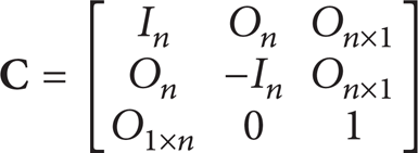
As is shown in Figure 7, a general multibody system can be considered as a system which consists of one tree subsystem and some closed-loop subsystems. After “cutting” at the junction of any two adjacent elements body 16 and hinge 19 in a closed-loop subsystem, a couple of “new boundaries” noted as z_16,0 and z_19,0, which are the same in nature, will emerge at the “cutting point.” Then, as shown in Figure 8, the original nontree system shown in Figure 7 will become a tree system with the same two “new boundaries” state vectors z_16,0 and z_19,0 at the “cutting points.” And the overall transfer equation of the general system with closed-loop subsystems can be deduced automatically by handwriting and by computer according to the method proposed in Section 4.3.

Figure 7:

Topology figure of a nontree system.

Figure 8:

Topology figure of a nontree system becoming a tree system after “cutting” the hinge 19.

It should be pointed out that either z_16,0 or z_19,0 is the input end state vector of elements 16 or 19 respectively. Thus, the internal force and internal moment in z_16,0 and z_19,0 are of the same quantities but with opposite direction due to the sign conventions, that is,

${\mathbf{U}}_{\text{all}}{\mathbf{z}}_{\text{all}}=\mathbf{0},$

(32)

where

$\begin{array}{c}{\mathbf{U}}_{\text{all}}=\left[\begin{array}{ccccc}-\mathbf{I}& {\mathbf{T}}_{\mathrm{15}-\mathrm{1}}& {\mathbf{T}}_{\mathrm{16}-\mathrm{1}}& {\mathbf{T}}_{\mathrm{17}-\mathrm{1}}& {\mathbf{T}}_{\mathrm{18}-\mathrm{1}}\\ \mathbf{O}& {\mathbf{G}}_{\mathrm{15}-\mathrm{9}}& {\mathbf{G}}_{\mathrm{16}-\mathrm{9}}& \mathbf{O}& \mathbf{O}\\ \mathbf{O}& \mathbf{O}& \mathbf{O}& {\mathbf{G}}_{\mathrm{17}-\mathrm{10}}& {\mathbf{G}}_{\mathrm{18}-\mathrm{10}}\\ \mathbf{O}& {\mathbf{G}}_{\mathrm{15}-\mathrm{4}}& {\mathbf{G}}_{\mathrm{16}-\mathrm{4}}& {\mathbf{G}}_{\mathrm{17}-\mathrm{4}}& {\mathbf{G}}_{\mathrm{18}-\mathrm{4}}\end{array}\right],\\ {\mathbf{z}}_{\text{all}}=\left[\begin{array}{c}{\mathbf{z}}_{\mathrm{1,0}}\\ {\mathbf{z}}_{\mathrm{15,0}}\\ {\mathbf{z}}_{\mathrm{16,0}}\\ {\mathbf{z}}_{\mathrm{17,0}}\\ {\mathbf{z}}_{\mathrm{18,0}}\end{array}\right].\end{array}$

(33)

n is equal to 3 for planar motion or 6 for spatial motion.

Considering the method proposed in Section 4.3 for a tree system, and regarding equation (34) concerned with the relationship between z_16,0 and z_19,0, the overall transfer equations of a general system with a closed-loop subsystem shown in Figure 8 can be obtained automatically by handwriting and by computer:

${\mathbf{z}}_{\mathrm{19,0}}=\mathbf{C}{\mathbf{z}}_{\mathrm{16,0}},$

(34)

where

$\mathbf{C}=\left[\begin{array}{ccc}{I}_n& O_n& O_{n\times \mathrm{1}}\\ O_n& -I_n& O_{n\times \mathrm{1}}\\ O_{\mathrm{1}\times n}& \mathrm{0}& \mathrm{1}\end{array}\right]$

(35)

Considering that z_19,0 can be explicitly expressed by z_16,0 due to equation (34), the overall transfer equation, the overall transfer matrix, and the overall state vectors equation (37) of the general system can be rewritten in the following form

${\mathbf{U}}_{\text{all}}{\mathbf{z}}_{\text{all}}=\mathbf{0}\mathbf{,}$

(36)

where

$\begin{array}{c}{\mathbf{U}}_{\text{all}}=\left[\begin{array}{ccccc}-\mathbf{I}& {\mathbf{T}}_{\mathrm{15}-\mathrm{1}}& {\mathbf{T}}_{\mathrm{16}-\mathrm{1}}& {\mathbf{T}}_{\mathrm{19}-\mathrm{1}}& {\mathbf{T}}_{\mathrm{18}-\mathrm{1}}\\ \mathbf{O}& {\mathbf{G}}_{\mathrm{15}-\mathrm{9}}& {\mathbf{G}}_{\mathrm{16}-\mathrm{9}}& \mathbf{O}& \mathbf{O}\\ \mathbf{O}& \mathbf{O}& \mathbf{O}& {\mathbf{G}}_{\mathrm{19}-\mathrm{10}}& {\mathbf{G}}_{\mathrm{18}-\mathrm{10}}\\ \mathbf{O}& {\mathbf{G}}_{\mathrm{15}-\mathrm{4}}& {\mathbf{G}}_{\mathrm{16}-\mathrm{4}}& {\mathbf{G}}_{\mathrm{19}-\mathrm{4}}& {\mathbf{G}}_{\mathrm{18}-\mathrm{4}}\\ \mathbf{O}& \mathbf{O}& \mathbf{C}& -\mathbf{I}& \mathbf{O}\end{array}\right],\\ {\mathbf{z}}_{\text{all}}=\left[\begin{array}{c}{\mathbf{z}}_{\mathrm{1,0}}\\ {\mathbf{z}}_{\mathrm{15,0}}\\ {\mathbf{z}}_{\mathrm{16,0}}\\ {\mathbf{z}}_{\mathrm{19,0}}\\ {\mathbf{z}}_{\mathrm{18,0}}\end{array}\right].\end{array}$

(37)

5. Automatic Deduction Theorem of Overall Transfer Equation

The following features of the overall transfer equation of a multibody system can be clearly concluded from equations (23), (24), (28), and (30). These features make up the theorem to deduce automatically the overall transfer equation as the following for tree system (1, 2), for chain system (1, 3), for closed-loop system (1, 3, 4), and for general system (1, 2, 5).

1. The state vectors involved in an overall transfer equation are the column matrix comprising the state vectors of all boundary ends of the system.

2. For a tree system, in the first line of the overall transfer matrix, the coefficient matrix of the state vector of root is a minus unit matrix, while each coefficient matrix of the state vector of a tip is the successive premultiplication of the transfer matrices of all elements in the transfer path from this tip to the root; besides the first line in the overall transfer matrix, all coefficient matrices of state vectors in the first column are zero matrices. Except the first line, in each row, each nonzero partitioned matrix corresponds to the coefficient matrix of the tip state vector, from which there is a transfer path to the input end of the element with multiple input ends. Each nonzero coefficient matrix of the state vector of a tip is the successive premultiplication of all transfer matrices of elements in the transfer path from this tip to the kth input end I _k of jth body element, which has more than two ends, then premultiplied by -H _j for k = 1 or premultiplied by H_{j,I k} for k = 2, 3, 4⋯L.

3. For a chain system, its overall transfer matrix is deduced automatically by successive premultiplication of the transfer matrices of all elements in the transfer path from the tip to the root of system. In fact, any chain system can be considered as a special example of the tree system in the case with only two boundary ends.

4. For a closed-loop system, its overall transfer equation is deduced automatically as the chain system, after treating the original system as the chain system by “cutting” a junction of any two adjacent elements and letting the couple of “cutting points” as the tip and root with the same state vectors of the chain system.

5. For a general system composed of one tree subsystem and some closed-loop subsystems, its overall transfer equation is deduced automatically as the tree system, after treating the original system as the tree system by “cutting” the junctions of any two adjacent elements in every closed-loop subsystem and letting every couple of “cutting points” as new “boundary ends” with the same state vectors of the tree system.

The theorem above is effective for various multi-rigid-body systems, chain multi-rigid-flexible-body systems, and any closed-loop multi-rigid-flexible-body systems and is effective for various tree multi-rigid-flexible-body systems and general multi-rigid-flexible-body systems if the bodies with more than two ends are rigid bodies. For more general systems including the flexible bodies with more than two ends, the theorem to deduce automatically overall transfer equation is undergoing study and will be discussed in another paper.

6. Numerical Examples

By comparison with Newton-Euler method, the numerical examples here are carried out to validate the proposed method.

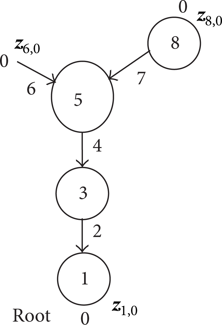
Example 1. A tree multi-rigid-flexible-body system moving in plane, as shown in Figure 9, consists of two fixed hinges, 2 and 4, two elastic hinges, 6 and 7, three rigid bodies, 1, 5, and 8, and one uniform beam element, 3, with three boundary ends. The simulation parameters are given as follows: m₁ = m₅ = m₈ = 7.8 kg, J_C,1 = J_C,5 = J_C,8 = 0.013 kg·m², l₃ = 3 m, EA₃ = 1000 N, ${\stackrel{-}{m}}_{\mathrm{3}}=\mathrm{0.78}\hspace{0.17em}\text{kg}/\text{m}$ , EI₃ = 166.67 N·m², K_x,6 = K_x,7 = 1000 N/m,K_y,6 = K_y,7 = 500 N/m, and K₆′ = K₇′ = 150 N·m/rad.

Figure 9:

Tree multi-rigid-flexible-body system.

According to the theorem to deduce automatically the overall transfer equation, the topology Figure of the system can be got as in Figure 10, and the overall transfer equation of above system is deduced automatically by handwriting and by computer as follows

$\begin{array}{c}{\mathbf{U}}_{\text{all}}{\mathbf{z}}_{\text{all}}=\mathbf{0}\\ {\mathbf{U}}_{\text{all}}=\left[\begin{array}{cccc}-\mathbf{I}& {\mathbf{T}}_{\mathrm{15}-\mathrm{1}}& {\mathbf{T}}_{\mathrm{16}-\mathrm{1}}+{\mathbf{T}}_{\mathrm{19}-\mathrm{1}}\mathbf{C}& {\mathbf{T}}_{\mathrm{18}-\mathrm{1}}\\ \mathbf{O}& {\mathbf{G}}_{\mathrm{15}-\mathrm{9}}& {\mathbf{G}}_{\mathrm{16}-\mathrm{9}}& \mathbf{O}\\ \mathbf{O}& \mathbf{O}& {\mathbf{G}}_{\mathrm{19}-\mathrm{10}}\mathbf{C}& {\mathbf{G}}_{\mathrm{18}-\mathrm{10}}\\ \mathbf{O}& {\mathbf{G}}_{\mathrm{15}-\mathrm{4}}& {\mathbf{G}}_{\mathrm{16}-\mathrm{4}}+{\mathbf{G}}_{\mathrm{19}-\mathrm{4}}\mathbf{C}& {\mathbf{G}}_{\mathrm{18}-\mathrm{4}}\end{array}\right],\\ {\mathbf{z}}_{\text{all}}=\left[\begin{array}{c}{\mathbf{z}}_{\mathrm{1,0}}\\ {\mathbf{z}}_{\mathrm{15,0}}\\ {\mathbf{z}}_{\mathrm{16,0}}\\ {\mathbf{z}}_{\mathrm{18,0}}\end{array}\right],\end{array}$

(38)

where the overall transfer matrix is

$\begin{array}{c}{\mathbf{T}}_{\mathrm{15}-\mathrm{1}}={\mathbf{U}}_{\mathrm{1}}{\mathbf{U}}_{\mathrm{2}}{\mathbf{U}}_{\mathrm{3}}{\mathbf{U}}_{\mathrm{4}}{\mathbf{U}}_{\mathrm{5}}{\mathbf{U}}_{\mathrm{7}}{\mathbf{U}}_{\mathrm{8}}{\mathbf{U}}_{\mathrm{9}}{\mathbf{U}}_{\mathrm{11}}{\mathbf{U}}_{\mathrm{15}},\\ {\mathbf{T}}_{\mathrm{16}-\mathrm{1}}={\mathbf{U}}_{\mathrm{1}}{\mathbf{U}}_{\mathrm{2}}{\mathbf{U}}_{\mathrm{3}}{\mathbf{U}}_{\mathrm{4}}{\mathbf{U}}_{\mathrm{5}}{\mathbf{U}}_{\mathrm{7}}{\mathbf{U}}_{\mathrm{8}}{\mathbf{U}}_{\mathrm{9,12}}{\mathbf{U}}_{\mathrm{12}}{\mathbf{U}}_{\mathrm{16}},\\ {\mathbf{T}}_{\mathrm{19}-\mathrm{1}}={\mathbf{U}}_{\mathrm{1}}{\mathbf{U}}_{\mathrm{2}}{\mathbf{U}}_{\mathrm{3}}{\mathbf{U}}_{\mathrm{4,6}}{\mathbf{U}}_{\mathrm{6}}{\mathbf{U}}_{\mathrm{10}}{\mathbf{U}}_{\mathrm{13}}{\mathbf{U}}_{\mathrm{17}}{\mathbf{U}}_{\mathrm{19}},\\ {\mathbf{T}}_{\mathrm{18}-\mathrm{1}}={\mathbf{U}}_{\mathrm{1}}{\mathbf{U}}_{\mathrm{2}}{\mathbf{U}}_{\mathrm{3}}{\mathbf{U}}_{\mathrm{4,6}}{\mathbf{U}}_{\mathrm{6}}{\mathbf{U}}_{\mathrm{10,14}}{\mathbf{U}}_{\mathrm{14}}{\mathbf{U}}_{\mathrm{18}},\\ {\mathbf{G}}_{\mathrm{15}-\mathrm{9}}=-{\mathbf{H}}_{\mathrm{9}}{\mathbf{U}}_{\mathrm{11}}{\mathbf{U}}_{\mathrm{15}},\\ {\mathbf{G}}_{\mathrm{16}-\mathrm{9}}={\mathbf{H}}_{\mathrm{9,12}}{\mathbf{U}}_{\mathrm{12}}{\mathbf{U}}_{\mathrm{16}},\\ {\mathbf{G}}_{\mathrm{19}-\mathrm{10}}=-{\mathbf{H}}_{\mathrm{10}}{\mathbf{U}}_{\mathrm{13}}{\mathbf{U}}_{\mathrm{17}}{\mathbf{U}}_{\mathrm{19}},\\ {\mathbf{G}}_{\mathrm{18}-\mathrm{10}}={\mathbf{H}}_{\mathrm{10,14}}{\mathbf{U}}_{\mathrm{14}}{\mathbf{U}}_{\mathrm{18}},\\ {\mathbf{G}}_{\mathrm{15}-\mathrm{4}}=-{\mathbf{H}}_{\mathrm{4}}{\mathbf{U}}_{\mathrm{5}}{\mathbf{U}}_{\mathrm{7}}{\mathbf{U}}_{\mathrm{8}}{\mathbf{U}}_{\mathrm{9}}{\mathbf{U}}_{\mathrm{11}}{\mathbf{U}}_{\mathrm{15}},\\ {\mathbf{G}}_{\mathrm{16}-\mathrm{4}}=-{\mathbf{H}}_{\mathrm{4}}{\mathbf{U}}_{\mathrm{5}}{\mathbf{U}}_{\mathrm{7}}{\mathbf{U}}_{\mathrm{8}}{\mathbf{U}}_{\mathrm{9,12}}{\mathbf{U}}_{\mathrm{12}}{\mathbf{U}}_{\mathrm{16}},\\ {\mathbf{G}}_{\mathrm{19}-\mathrm{4}}={\mathbf{H}}_{\mathrm{4,6}}{\mathbf{U}}_{\mathrm{6}}{\mathbf{U}}_{\mathrm{10}}{\mathbf{U}}_{\mathrm{13}}{\mathbf{U}}_{\mathrm{17}}{\mathbf{U}}_{\mathrm{19}},\\ {\mathbf{G}}_{\mathrm{18}-\mathrm{4}}={\mathbf{H}}_{\mathrm{4,6}}{\mathbf{U}}_{\mathrm{6}}{\mathbf{U}}_{\mathrm{10,14}}{\mathbf{U}}_{\mathrm{14}}{\mathbf{U}}_{\mathrm{18}}.\end{array}$

(39)

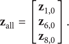
State vectors of all boundary ends are

${\mathbf{U}}_{\text{all}}{\mathbf{z}}_{\text{all}}=\mathbf{0}\mathbf{,}$

(40)

According to the proposed sign conventions, we know that

${\mathbf{U}}_{\text{all}}=\left[\begin{array}{ccc}-\mathbf{I}& {\mathbf{T}}_{\mathrm{6}-\mathrm{1}}\mathrm{\hspace{0.17em}\hspace{0.17em}}& {\mathbf{T}}_{\mathrm{8}-\mathrm{1}}\\ \mathbf{O}& {\mathbf{G}}_{\mathrm{6}-\mathrm{5}}& {\mathbf{G}}_{\mathrm{8}-\mathrm{5}}\end{array}\right].$

(41)

where z_1,0 is state vector of root, z_6,0 and z_8,0 are the state vectors of tips, and U₁, U₂, U₃, U₄, U₅, U_5,7, U₆, U₇, and U₈ are the transfer matrices of body 1, fixed hinge 2, uniform beam 3, fixed hinge 4, body 5, elastic hinge 6, elastic hinge 7, and body 8. All of the transfer matrices can be found directly from the library of transfer matrices in [19, 30].

Figure 10:

Topology figure of the system.

There are boundary conditions of the system

${\mathbf{z}}_{\text{all}}=\left[\begin{array}{c}{\mathbf{z}}_{\mathrm{1,0}}\\ {\mathbf{z}}_{\mathrm{6,0}}\\ {\mathbf{z}}_{\mathrm{8,0}}\end{array}\right].$

(42)

The system experiences a step upward force at the mass center of body element 1 at time instant zero, while the initial displacement and velocity of the whole system are zero. The computational results of the system dynamics obtained by the proposal method and by Newton-Euler method are shown in Figure 11. It can be seen from Figure 11 that the computational results obtained by the above two methods have good agreements.

Figure 11:

Computational results of the angle of the right end of the beam.

Example 2. A multi-rigid-body system containing a close loop moving in plane is shown in Figure 12. The planar rigid bodies (numbered 1, 3, 5, 7, 9, 11, and 13) are connected by pin hinges (numbered 2, 4, 6, 8, 10, 12, and 14), and rigid body 1 is connected with the ground by a smooth pin. Each rigid body has the identical dynamics parameter as m = 1 kg and J _C = (1/6) kg·m².

Figure 12:

A general system moving in plane.

By “cutting” at the junction of body 9 and hinge 14 and following the proposed theorem, topology Figure of the system can be drawn in Figure 13. And the overall transfer equation of the system can be derived automatically as

$\begin{array}{c}{\mathbf{T}}_{\mathrm{6}-\mathrm{1}}={\mathbf{U}}_{\mathrm{1}}{\mathbf{U}}_{\mathrm{2}}{\mathbf{U}}_{\mathrm{3}}{\mathbf{U}}_{\mathrm{4}}{\mathbf{U}}_{\mathrm{5}}{\mathbf{U}}_{\mathrm{6}},\\ {\mathbf{T}}_{\mathrm{8}-\mathrm{1}}={\mathbf{U}}_{\mathrm{1}}{\mathbf{U}}_{\mathrm{2}}{\mathbf{U}}_{\mathrm{3}}{\mathbf{U}}_{\mathrm{4}}{\mathbf{U}}_{\mathrm{5,7}}{\mathbf{U}}_{\mathrm{7}}{\mathbf{U}}_{\mathrm{8}},\\ {\mathbf{G}}_{\mathrm{6}-\mathrm{5}}=-{\mathbf{H}}_{\mathrm{5}}{\mathbf{U}}_{\mathrm{6}},\\ {\mathbf{G}}_{\mathrm{8}-\mathrm{5}}={\mathbf{H}}_{\mathrm{5,7}}{\mathbf{U}}_{\mathrm{7}}{\mathbf{U}}_{\mathrm{8}},\end{array}$

(43)

where the overall transfer matrix takes the form:

$\begin{array}{c}{\mathbf{z}}_{\mathrm{1,0}}={\left[\begin{array}{ccccccc}\ddot{x}& \ddot{y}& \mathrm{\hspace{0.17em}\hspace{0.17em}}{\ddot{\theta }}_z& \mathrm{0}& \mathrm{0}& \mathrm{0}& \mathrm{1}\end{array}\right]}_{\mathrm{1,0}}^T,\\ {\mathbf{z}}_{\mathrm{6,0}}={\left[\begin{array}{ccccccc}\mathrm{0}& \mathrm{0}& \mathrm{0}& m_z& q_x& q_y& \mathrm{1}\end{array}\right]}_{\mathrm{6,0}}^T,\\ {\mathbf{z}}_{\mathrm{8,0}}={\left[\begin{array}{ccccccc}\ddot{x}& \ddot{y}& {\ddot{\theta }}_z& \mathrm{0}& \mathrm{0}& \mathrm{0}& \mathrm{1}\end{array}\right]}_{\mathrm{8,0}}^T.\end{array}$

(44)

${\mathbf{U}}_{\text{all}}{\mathbf{z}}_{\text{all}}=\mathbf{0}\mathbf{,}$

(45)

State vectors of all boundary ends are

${\mathbf{z}}_{\text{all}}\mathbf{=}\left[\begin{array}{c}{\mathbf{z}}_{\mathrm{1,0}}\\ {\mathbf{z}}_{\mathrm{9,0}}\\ {\mathbf{z}}_{\mathrm{14,0}}\end{array}\right].$

(46)

According to the proposed sign conventions, one can acquire

$\begin{array}{c}{\mathit{T}}_{\mathrm{9}-\mathrm{1}}={\mathit{U}}_{\mathrm{1}}{\mathit{U}}_{\mathrm{2}}{\mathit{U}}_{\mathrm{3}}{\mathit{U}}_{\mathrm{4}}{\mathit{U}}_{\mathrm{5}}{\mathit{U}}_{\mathrm{6}}{\mathit{U}}_{\mathrm{7}}{\mathit{U}}_{\mathrm{8}}{\mathit{U}}_{\mathrm{9}},\\ {\mathit{T}}_{14-1}={\mathit{U}}_1{\mathit{U}}_2{\mathit{U}}_{\mathrm{3,10}}{\mathit{U}}_{10}{\mathit{U}}_{11}{\mathit{U}}_{12}{\mathit{U}}_{13}{\mathit{U}}_{14},\\ {\mathit{G}}_{\mathrm{9}-\mathrm{3}}=-{\mathit{H}}_{\mathrm{3}}{\mathit{U}}_{\mathrm{4}}{\mathit{U}}_{\mathrm{5}}{\mathit{U}}_{\mathrm{6}}{\mathit{U}}_{\mathrm{7}}{\mathit{U}}_{\mathrm{8}}{\mathit{U}}_{\mathrm{9}},\\ {\mathit{G}}_{14-3}={\mathit{H}}_{\mathrm{3,10}}{\mathit{U}}_{10}{\mathit{U}}_{11}{\mathit{U}}_{12}{\mathit{U}}_{13}{\mathit{U}}_{14}.\end{array}$

(47)

z_1,0 is the state vector of the root; z_9,0 and z_14,0 are the state vectors of tips emerging after the “cutting.” U₁, U₃, U_3,10, U₅, U₇, U₉, U₁₁, and U₁₃ are the transfer matrices of the corresponding planar rigid bodies. U₂, U₄, U₆, U₈, U₁₀, U₁₂, and U₁₄ are transfer matrices of the corresponding planar pin hinges.

Figure 13:

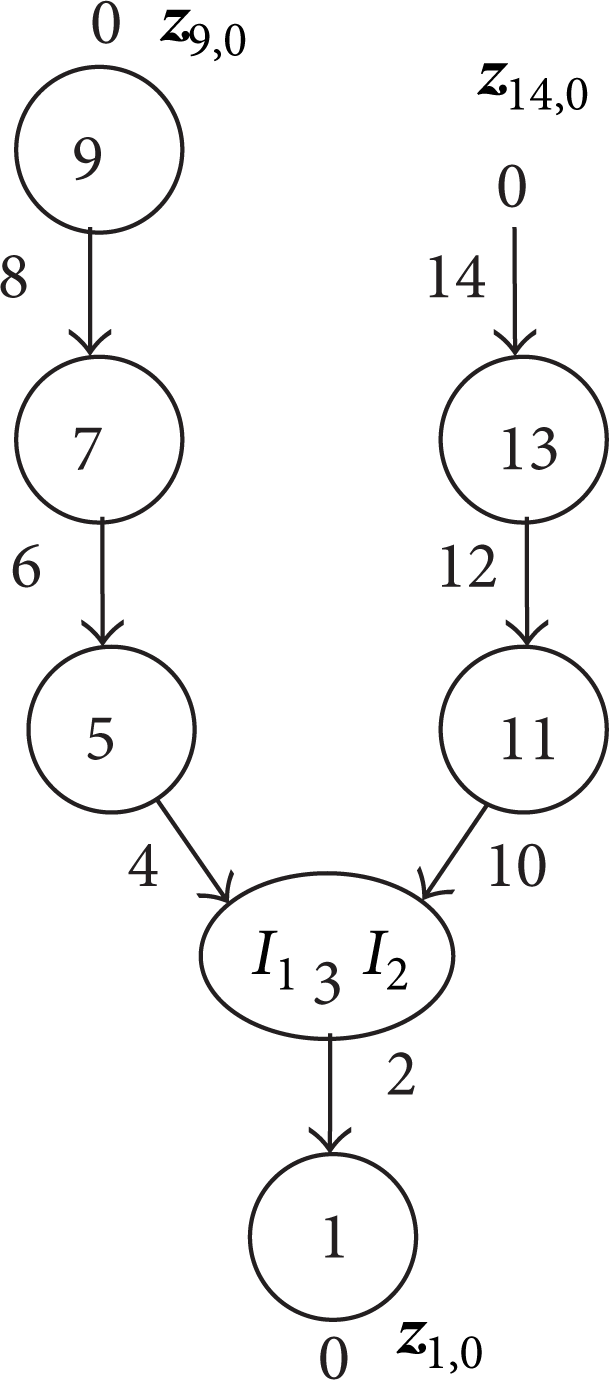
Topology figure of the system.

There are boundary conditions of the system:

${\mathbf{z}}_{\mathrm{1,0}}={\left[\begin{array}{ccccccc}\mathrm{0}& \mathrm{0}& {\ddot{\theta }}_z& \mathrm{0}& q_x& q_y& \mathrm{1}\end{array}\right]}_{\mathrm{1,0}}^T.$

(48)

The initial angle of rigid body 1 is (π/6) rad and the relative angles of pin hinges (numbered 2, 4, 6, 8, 10, 12, and 14) are all zero. The system moves from the rest under the effect of gravity. The computational results of the system dynamics are obtained by the proposal method and by Newton-Euler method. The time history of rigid body 1's angle is exhibited in Figure 14, which shows that the computational results obtained by the above two methods have good agreements.

Figure 14:

Computational results of the angle of rigid body 1.

7. Conclusions

Based on MSTMM and the features of the overall transfer equations of multibody systems with various topological structures, including chain systems, closed-loop systems, tree systems, general systems composed of one tree subsystem, and some closed-loop subsystems, the theorem to deduce automatically the overall transfer equation by handwriting and by computer is presented. Formulations of the proposed theorem as well as two numerical examples are given to verify the theorem. This makes it possible to program large-scale software for MSD with much higher computational speed and much higher programming.

Conflict of Interests

The authors declare that there is no conflict of interests regarding the publication of this paper.