Sage Journals: Discover world-class research

Abstract

A new algorithm based on the standard optimal homotopy asymptotic method, namely, the predictor optimal homotopy asymptotic method (POHAM), is proposed to predict the multiplicity of the solutions of nonlinear differential equations with boundary conditions. This approach is successfully implemented to obtain multiple solutions of a mixed convection flow model in a vertical channel and a nonlinear model arising in heat transfer. A new technique for obtaining the initial guess to accelerate the convergence of the series solution is presented.

1. Introduction

The study of the existence of multiple solutions for nonlinear differential equations has drawn a lot of attention in the last few years [1, 2]. Multiple solution for nonlinear boundary value problems via homotopy analysis method was investigated by several papers, for example, Liao [3, 4], Li and Liao [5], Xu and Liao [6]. Moreover, Abbasbandy and Shivanian [7] presented a kind of analytical method, namely, predictor homotopy analysis method (PHAM) to predict the multiplicity of the solutions of nonlinear differential equations with boundary conditions. Also, Alomari et al. [8] used the PHAM to find the multiple solutions of fractional boundary value problem (FBVP).

In the last few years, optimal homotopy asymptotic method (OHAM) has been introduced and developed by Marinca and Herişanu [9 –12] and has been applied successfully to many strongly nonlinear problems [13 –16]. Iqbal et al. [17] obtained OHAM solutions to linear and nonlinear Klein-Gordan equations, Anakira et al. [18] used OHAM for solving singular two-point boundary value problems, and Alomari et al. [19] employed OHAM to obtain approximate solution of nonlinear system of boundary value problems arising in fluid flow problems. Moreover, Idrees et al. [20, 21] and Mabood et al. [22, 23] have applied OHAM effectively to different higher-order boundary values problems.

The main aim of this paper is to present a type of analytical method, namely, the predictor optimal homotopy asymptotic method (POHAM), to predict the multiplicity of the solutions of the nonlinear differential equations with boundary conditions by using one auxiliary linear operator, one auxiliary function, and one initial guess. This paper is composed as follows. In Section 2, the structure of POHAM is formulated for finding multiple solutions of nonlinear differential equations. In Section 3, we present two numerical examples, and finally, we give the conclusion of this study in Section 4.

2. The Predictor Optimal Homotopy Asymptotic Method (POHAM)

Consider the following differential equation:

L (y (x)) + g (x) + N (y (x)) = 0, x \in Ω

(1)

with boundary conditions:

B (y, \frac{\partial y}{\partial η}) = 0, x \in Γ,

(2)

where L is the linear operator, N is the linear or nonlinear operator, g(x) is a known function, B is a boundary operator, and Γ is the boundary of the domain Ω. The key step of POHAM depends on the fact that the boundary value problem (1) and (2) should be transcribed to an equivalent problem so that the boundary condition (2) involves an unknown parameter, the so-called prescribed parameter δ, and is decomposed into

B^{'} (y, δ, \frac{\partial y}{\partial η}) = 0, x \in Γ, y (α) = β,

(3)

where y(α) = β is the forcing condition that resulted from the original condition (2) and B′ is the remaining boundary operator that contains the prescribed parameter δ. As it will be noticed, the parameter δ with the help of convergence controller parameter C_i's will play a significant role to realize the multiplicity of solutions. Now, we construct the POHAM on (1) and (3). By using a homotopy map h(v(x,δ;q);q):Ω × [0, 1]→R which satisfies

\begin{matrix} (1 - q) [L (v (x, δ; q)) - y_{0} (x; δ)] = H (q) [L (v (x, δ; q)) + g (x) + N (v (x, δ; q))], \\ B^{'} (v (x, δ; q), \frac{\partial v (x, δ; q)}{\partial x}) = 0, \end{matrix}

(4)

where x∈R, q∈[0, 1] is an embedding parameter, H(q) is a nonzero auxiliary function for q≠0, H(0) = 0, and v(x,δ;q) is an unknown function. Obviously, when q = 0 and q = 1, it holds that v(x,δ;0) = y₀(x;δ) and v(x,δ;1) = y(x), respectively. Thus, as q varies from 0 to 1, the solution v(x,δ;q) approaches from y₀(x;δ) to y(x), where y₀(x;δ) is the initial guess that satisfies the linear operator and the boundary conditions:

B^{'} (y_{0}, \frac{d y_{0}}{d x}) = 0 .

(5)

Next, we choose the auxiliary function H(q) in the form

H (q) = q C_{1} + q^{2} C_{2} + q^{3} C_{3} + \dots,

(6)

where C₁,C₂,C₃,… are constants which will be determined later. To obtain an approximate solution, we expand v(x,δ;q) in Taylor's series about q in the following manner:

v (x, δ; q) = y_{0} (x, δ) + \sum_{k = 1}^{\infty} ‍ y_{k} (x, δ) q^{k} .

(7)

Substituting (7) into (4) and equating the coefficient of like powers of p, we obtain the following linear equations, by defining the vector ${\vec{y}}_{k} = {y_{0} (x), y_{1} (x), \dots y_{k} (x)}$ . The first- and second-order problems are given as

\begin{matrix} L (y_{1} (x, δ)) + g (x) = C_{1} N_{0} (y_{0} (x, δ)), \\ B^{'} (y_{1}, \frac{d y_{1}}{d x}) = 0, \end{matrix}

(8)

\begin{matrix} L (y_{2} (x, δ)) - L (y_{1} (x, δ)) = C_{2} N_{0} (y_{0} (x, δ)) + C_{1} [L (y_{1} (x)) + N_{1} (y_{0} (x, δ), y_{1} (x, δ))], \\ B^{'} (y_{2}, \frac{d y_{2}}{d x}) = 0 . \end{matrix}

(9)

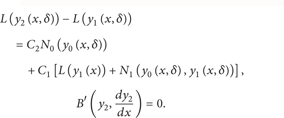
The general governing equations for y_k(x,δ) are

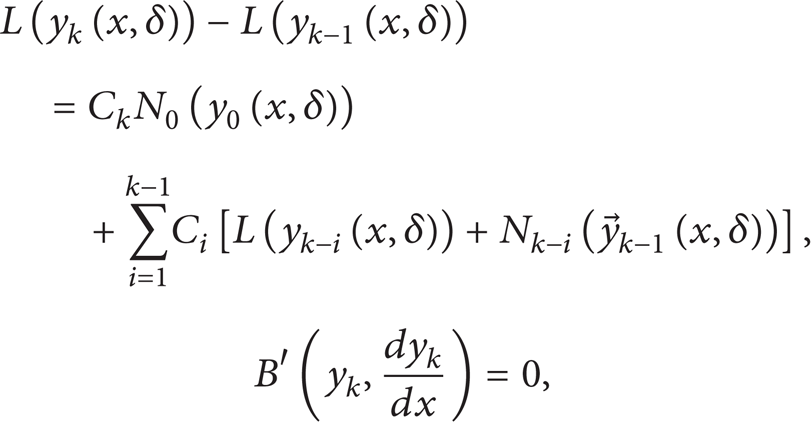
\begin{matrix} L (y_{k} (x, δ)) - L (y_{k - 1} (x, δ)) = C_{k} N_{0} (y_{0} (x, δ)) + \sum_{i = 1}^{k - 1} ‍ C_{i} [L (y_{k - i} (x, δ)) + N_{k - i} ({\vec{y}}_{k - 1} (x, δ))], \\ B^{'} (y_{k}, \frac{d y_{k}}{d x}) = 0, \end{matrix}

(10)

where k = 2, 3,… and

N_{m} ({\vec{y}}_{m - 1}, x, δ) = \frac{1}{(m - 1)!} {|\frac{\partial^{m - 1} N [\sum_{n = 0}^{\infty} ‍ y_{n} (x, δ) q^{n}]}{\partial q^{m - 1}}|}_{q = 0} .

(11)

The convergence of the series (7) depends upon the auxiliary convergent control parameters C₁,C₂,C₃,…. If it is convergent at q = 1, then

v (x, C_{i}) = y_{0} (x, δ) + \sum_{k = 1}^{\infty} ‍ y_{k} (x, C_{1}, C_{2}, \dots, C_{k}) .

(12)

Thus the mth-order solution is given by

\tilde{y} (x, δ, C_{1}, C_{2}, C_{3}, \dots, C_{m}) = y_{0} (x, δ) + \sum_{i = 1}^{m} ‍ y_{i} (x, δ, C_{1}, C_{2}, \dots, C_{i}) .

(13)

Substituting (12) into (1) yields the following residual:

R (x, δ, C_{1}, C_{2}, C_{3}, \dots, C_{m}) = L (\tilde{y} (x, δ, C_{1}, C_{2}, C_{3}, \dots, C_{m})) + g (x) + N (\tilde{y} (x, δ, C_{1}, C_{2}, C_{3}, \dots, C_{m})) .

(14)

If R = 0, then $\tilde{y}$ will be the exact solution. Generally, such a case will not arise for nonlinear problems, but we can minimize the functional

J (C_{1}, C_{2}, C_{3}, \dots, C_{m}) = \int_{a}^{b} ‍ R^{2} (x, δ, C_{1}, C_{2}, C_{3}, \dots, C_{m}) d x,

(15)

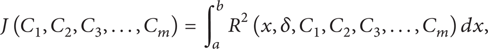
where a and b are two values, depending on the problem. The unknown convergent control parameters C_i (i = 1, 2, 3,…, m) and the so-called prescribed parameter δ can be identified from the conditions

\frac{\partial J}{\partial C_{1}} = \frac{\partial J}{\partial C_{2}} = \dots = \frac{\partial J}{\partial C_{m}} = 0, \tilde{y} (α) = β .

(16)

With those known convergent control parameters, the approximate solution (of order m) is determined. Note that the force condition plays a significant role to determine the multiple solutions.

3. Applications

In this section, we will present two examples to demonstrate the effectiveness and high precision of present method.

3.1. Example 1

The first example comes from a mixed convection flow problem in a vertical channel studied by Barletta et al. [24]. The two walls are assumed to be isothermal. Furthermore, the effect of viscous dissipation is taken into account and the Boussinesq approximation is adopted. By employing appropriate dimensionless quantities, the governing equations were reduced to the following nonlinear fourth-order ordinary differential equation for the dimensionless velocity field (cf. [7, 24])

\frac{d^{4} y}{d x^{4}} = \frac{E}{16} {(\frac{d y}{d x})}^{2},

(17)

subject to the boundary conditions

y (1) = y^{'} (0) = y^{'''} (0) = 0, \int_{0}^{1} ‍ y (x) d x = 1,

(18)

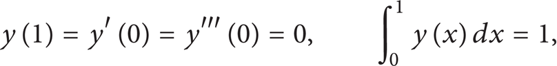
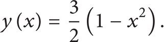
where y is the dimensionless velocity, x is the transversal coordinate, and E is a constant. In the case E = 0, (17) and (18) are easily solved and admit a unique solution

y (x) = \frac{3}{2} (1 - x^{2}) .

(19)

It was shown by perturbation method and a numerical method that (17) and (18) admit multiple solutions to any given E in the interval (–∞, 0)∪(0,E_max) where E_max = 228.128 (cf. [24, 25]).

To find out the multiple solutions, we consider (17) and (18) and suppose that y″(0) = δ, where δ is a prescribed parameter that plays an important role in recognizing the multiplicity of solutions, so that the problem becomes

\frac{d^{4} y}{d x^{4}} = \frac{E}{16} {(\frac{d y}{d x})}^{2},

(20)

subject to the boundary conditions

y (1) = y^{'} (0) = y^{'''} (0) = 0, y^{′′} (0) = δ,

(21)

with additional force condition

\int_{0}^{1} ‍ y (x) d x = 1 .

(22)

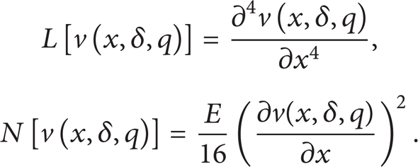
According to POHAM, we chose the linear and nonlinear operator as follows, respectively:

\begin{matrix} L [v (x, δ, q)] = \frac{\partial^{4} v (x, δ, q)}{\partial x^{4}}, \\ N [v (x, δ, q)] = \frac{E}{16} {(\frac{\partial v (x, δ, q)}{\partial x})}^{2} . \end{matrix}

(23)

Under the rule of the solution expression and according to conditions (21) it is easy to choose

y_{0} (x, δ) = \frac{δ}{2} (x^{2} - 1),

(24)

as initial guess. The first-order problem is obtained from (8) as follows:

\begin{matrix} y_{1}^{(4)} (x, δ) = \frac{- E x^{2} δ^{2} C_{1}}{16}, \\ y_{1}^{'} (0) = y_{1}^{'''} (0) = y_{1} (1) = y_{1}^{′′} (0) = 0 . \end{matrix}

(25)

From (9) the second-order problem is defined as

\begin{matrix} y_{2}^{′′′′} (x, δ) = - \frac{E x^{2} δ^{2} C_{2}}{16} - \frac{E x δ C_{1}}{8} y_{1}^{'} (x, δ) + y_{1}^{′′′′} (x, δ) + C_{1} y_{1}^{′′′′} (x, δ), \\ y_{2}^{'} (0) = y_{2}^{'''} (0) = y_{2} (1) = y_{2}^{′′} (0) = 0 . \end{matrix}

(26)

By using (10) for k = 3 and k = 4, the third- and fourth-order problems are given, respectively, as follows:

\begin{matrix} y_{3}^{′′′′} (x, δ) = y_{2}^{′′′′} (x, δ) - \frac{1}{16} E x^{2} δ^{2} C_{3} - \frac{1}{8} E x δ C_{2} y_{1}^{'} (x, δ) - \frac{1}{16} E C_{1} {(y_{1}^{'})}^{2} (x, δ) - \frac{1}{8} E x δ C_{1} y_{2}^{'} (x, δ) - C_{2} y_{1}^{′′′′} (x, δ) - C_{1} y_{2}^{′′′′} (x, δ), \\ y_{3}^{'} (0) = y_{3}^{'''} (0) = y_{3} (1) = y_{3}^{′′} (0) = 0, \\ y_{4}^{′′′′} (x, δ) = C_{2} y_{2}^{′′′′} (x, δ) + y_{3}^{′′′′} (x, δ) + C_{1} y_{3}^{′′′′} (x, δ) - \frac{E x^{2} δ^{2} C_{4}}{16} - \frac{E x δ C_{3}}{8} y_{1}^{'} (x) - \frac{E C_{2}}{16} {(y_{1}^{'})}^{2} (x, δ) - \frac{E x δ C_{2}}{16} y_{2}^{'} (x, δ) - \frac{E C_{1}}{8} y_{1}^{'} (x, δ) y_{2}^{'} (x, δ) - \frac{E x δ C_{1}}{8} y_{3}^{'} (x, δ) + C_{3} y_{1}^{′′′′} (x, δ), \\ y_{4}^{'} (0) = y_{4}^{'''} (0) = y_{4} (1) = y_{4}^{′′} (0) = 0 . \end{matrix}

(27)

Substituting the solution of (25)–(27) into (13) yields the fourth-order approximate solutions (m = 4) for (20) and (21):

\tilde{y} (x, δ) = y_{0} (x, δ) + y_{1} (x, δ) + y_{2} (x, δ) + y_{3} (x, δ) + y_{4} (x, δ) .

(28)

Substituting the fourth-order approximate solution (28) into (14) yields the residual error and the functional J, respectively:

\begin{matrix} R \tilde{y} (x, δ) = {\tilde{y}}^{′′′′} (x, δ) - \frac{E}{16} {({\tilde{y}}^{'} (x, δ))}^{2}, \\ J (C_{1}, C_{2}, C_{3}, C_{4}) = \int_{0}^{1} ‍ R^{2} (x, δ, C_{1}, C_{2}, C_{3}, C_{4}) d x, \end{matrix}

(29)

with the additional force condition

\int_{0}^{1} ‍ y (x) d x = 1 .

(30)

Now, to be specific, we consider two cases consisting of E = 20 and E = −20, with a prescribed parameter δ as a function of the convergence controller parameter. From conditions (16), the values of the convergent control parameters C_i's are obtained based on the values of the prescribed parameter δ as presented in Table 1. We plot the multiple (dual) solutions in Figure 1. It is worth to mention here that Figure 1(a) indicates the existence of two solutions for E = 20 so that u″(0) = −3.08411 for the first branch of the solution and u″(0) = −161.726 for the second branch of the solution. The same procedure was done for case E = −20, as we can see in Figure 1(b). It is obviouse that the results being obtained by using fourth terms POHAM approximate solution is to an extent identical compared with the 25th terms PHAM approximate solution [7]. This means that the POHAM solution reveals very good agreement with PHAM solution in few terms which prove the validity and the efficiency of our procedure in solving strongly nonlinear problems.

Table 1:

Values of C_i's corresponding to the prescribed parameter δ for Example 1.

	E = 20		E = −20
	δ₁ = −3.09773	δ₂ = −161.726	δ₁ = −2.92300	δ₂ = 170.039

C1	−1.63557 × 10⁻¹⁵	−0.738509	−1.07453	−0.438751
C2	5.54432 × 10⁻¹⁵	−0.695483	0.005063	−0.592496
C3	1.05665 × 10⁻¹⁵	−0.617731	−0.000767	0.259233
C4	−1.14066	−0.836292	−0.088768	−0.518427

Figure 1:

Multiple solutions of (20) and (21) for (a) E = 20 and (b) E = −20.

3.2. Example 2

Our second example comes from the heat conduction problem for a fin with heat transfer coefficient varying as a power-law function of temperature considered by Chang [26]. The rate of heat transfer on a solid surface can be enhanced by fins. In the mathematical modelling, Chang [26] considered a straight fin of finite length and uniform cross-section area. The fin surface is exposed to a prescribed ambient temperature. The dimensionless equation for the one-dimensional steady state heat conduction is given as (cf. [7, 26])

\frac{d^{2} y}{d x^{2}} - N^{2} y^{n + 1} = 0,

(31)

subject to the boundary conditions

y^{'} (0) = 0, y (1) = 1,

(32)

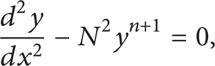
where N is the convective-conductive parameter. It was shown that the problem (31) and (32), when −4 ≤ n ≤ −2, either admit multiple solutions or does not admit any solution for a given convective-conductive parameter N [27]. In particular, suppose that N = 2/5 and n = −4; then (31) is converted into

y^{′′} (x) y^{3} (x) - \frac{4}{25} = 0,

(33)

subject to the boundary conditions

y^{'} (0) = 0, y (0) = δ,

(34)

where δ is the temperature of the fin tip and is determined by the rule of multiplicity of the solutions. With the additional force condition

y (1) = 1 .

(35)

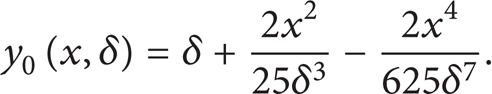
The exact multiple (dual) solutions of this problem are given by

\frac{5}{2} λ \sqrt{y^{2} (x) - λ^{2}} = x,

(36)

where y(0) = λ is represented by two values: λ = 0.4472135954 for the first branch of the solution and λ = 0.8944271909 for the second branch of the solution. The linear operator can be defined as

L [v (x, δ, q)] = \frac{\partial^{2} v (x, δ, q)}{\partial x^{2}} .

(37)

It is straightforward to choose

y_{0} (x) = δ

(38)

as the initial guess. The first four order problems are as follows.

First-order problem given by (8):

\begin{matrix} y_{1}^{′′} (x, δ) = - \frac{4 C_{1}}{25}, \\ y_{1} (0) = 0, y_{1}^{'} (0) = 0 . \end{matrix}

(39)

Second-order problem given by (9):

\begin{matrix} y_{2}^{′′} (x, δ) = y_{1}^{′′} (x, δ) + δ^{3} C_{1} y_{1}^{′′} (x, δ) - \frac{4 C_{2}}{25}, \\ y_{2} (0) = 0, y_{2}^{'} (0) = 0 . \end{matrix}

(40)

Third-order problem obtained from (10) for k = 3:

\begin{matrix} y_{3}^{′′} (x, δ) = δ^{3} C_{2} y_{1}^{′′} (x, δ) + 3 δ^{2} C_{1} y_{1} (x, δ) y_{1}^{′′} (x, δ) + y_{2}^{′′} (x, δ) + δ^{3} C_{1} y_{2}^{′′} (x, δ) - \frac{4 C_{3}}{25}, \\ y_{3} (0) = 0, y_{3}^{'} (0) = 0 . \end{matrix}

(41)

Fourth-order problem obtained from (10) for k = 4:

\begin{matrix} y_{4}^{′′} (x, δ) = δ^{3} C_{3} y_{1}^{′′} (x, δ) + 3 δ^{2} C_{2} y_{1} (x, δ) y_{1}^{′′} (x, δ) + 3 δ C_{1} {(y_{1} (x, δ))}^{2} y_{1}^{′′} (x, δ) + 3 δ^{2} C_{1} y_{2} (x, δ) y_{1}^{′′} (x, δ) + δ^{3} C_{2} y_{2}^{′′} (x, δ) + 3 δ^{2} C_{1} y_{1} (x, δ) y_{2}^{′′} (x, δ) + y_{3}^{′′} (x, δ) + δ^{3} C_{1} y_{3}^{′′} (x, δ) - \frac{4 C_{4}}{25}, \\ y_{4} (0) = 0, y_{4}^{'} (0) = 0 . \end{matrix}

(42)

The fourth-order POHAM approximate analytical solution obtained by substituting the solutions of (39)–(42) into (13) for m = 4:

\tilde{y} (x, δ) = y_{0} (x, δ) + y_{1} (x, δ) + y_{2} (x, δ) + y_{3} (x, δ) + y_{4} (x, δ) .

(43)

Using (43) into (14) yields the residual error and the functional J, respectively:

\begin{matrix} R \tilde{y} (x, δ) = \tilde{y} (x, δ) {\tilde{y}}^{3} (x, δ) - \frac{4}{25}, \\ J (C_{1}, C_{2}, C_{3}, C_{4}) = \int_{0}^{1} ‍ R^{2} (x, δ, C_{1}, C_{2}, C_{3}, C_{4}) d x, \end{matrix}

(44)

with the additional force condition

y (1) = 1 .

(45)

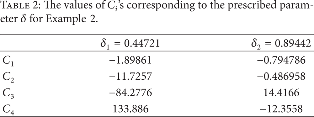
The optimal values of the convergent control parameters C_i's obtained from conditions (16) corresponding to the values of the prescribed parameters δ₁ = 0.44721 and δ₂ = 0.89442 are as shown in Table 2. Obviously, multiple (dual) solutions exist and are plotted in Figure 2. It is wroth to mention here that Figure 2 indicates existence of two solutions: y(0) = 0.44721 for the first branch of the solution and y(0) = 0.89442 for the second branch of the solution.

Table 2:

The values of C_i's corresponding to the prescribed parameter δ for Example 2.

	δ₁ = 0.44721	δ₂ = 0.89442

C1	−1.89861	−0.794786
C2	−11.7257	−0.486958
C3	−84.2776	14.4166
C4	133.886	−12.3558

Figure 2:

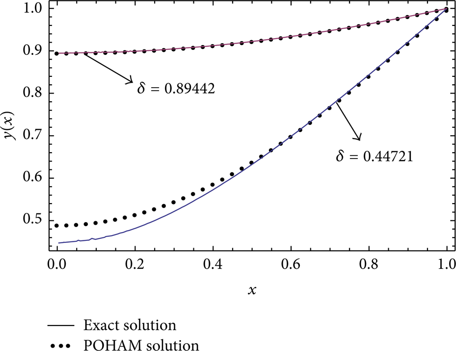
Comparison between the fourth-order POHAM approximate solutions and the exact multiple (dual) solutions (36) for Example 2.

We notice that POHAM does not yield good agreement with the exact solutions for both cases shown in Figure 2. To improve the accuracy we can use a new initial guess. We use the standard homotopy analysis method (HAM) for two terms and employ the Least Squares method to define the optimal values of $ħ = 1 / δ^{3}$ . This yields the following new initial guess:

y_{0} (x, δ) = δ + \frac{2 x^{2}}{25 δ^{3}} - \frac{2 x^{4}}{625 δ^{7}} .

(46)

With this new initial guess and taking only three terms in POHAM series solution we obtain δ₁ = 0.44721 and δ₂ = 0.89442 as shown in Table 3. Figure 3 demonstrates the good accuracy of the POHAM multiple solutions. In this regard, it is very important to notify that this result is obtained by using three terms POHAM approximate solution compared with 40th terms PHAM approximate solution [7]. This implies that this method could be useful and effective in solving nonlinear differential equations and it can converge to the exact solution in few terms.

Table 3:

The values of C_i's corresponding to the new initial guess and the prescribed parameter δ for Example 2.

	δ₁ = 0.44721	δ₂ = 0.89442

C1	−2.53856	−0.828156
C2	2.24311	−0.402523
C3	−1.8665	0.157102

Figure 3:

Comparison between the third-order POHAM approximate solutions and the exact multiple (dual) solutions (36) for Example 2.

4. Conclusions

In this work, a new algorithm called the predictor optimal homotopy asymptotic method (POHAM) is employed to find approximate solutions of nonlinear differential equations. POHAM has been shown to be a reliable method for obtaining multiple (dual) solutions of nonlinear differential equations which arise in fluid mechanics. General framework for the multiple solutions is given without any need to perturbation methods, special discretization, or transformation. The validity and applicability of this procedure is independent whether there exists a small parameter in the governing equations or not.

Conflict of Interests

The authors declare that there is no conflict of interests regarding the publication of this paper.

References

Zhang

and Sun

, “Multiple positive solutions of singular second-order m-point boundary value problems,” Journal of Mathematical Analysis and Applications, vol. 317, no. 2, pp. 442–447, 2006.

Feng

, and Jiang

, “Multiple positive solutions for m-point boundary-value problems with a one-dimensional p-Laplacian,” Nonlinear Analysis: Theory, Methods and Applications, vol. 68, no. 8, pp. 2269–2279, 2008.

Liao

, “Finding multiple solutions of nonlinear problems by means of the homotopy analysis method,” Journal of Hydrodynamics, vol. 18, no. 3, pp. 54–56, 2006.

Liao

, “A new branch of solutions of boundary-layer flows over an impermeable stretched plate,” International Journal of Heat and Mass Transfer, vol. 48, no. 12, pp. 2529–2539, 2005.

and Liao

S.-J.

, “An analytic approach to solve multiple solutions of a strongly nonlinear problem,” Applied Mathematics and Computation, vol. 169, no. 2, pp. 854–865, 2005.

and Liao

S.-J.

, “Dual solutions of boundary layer flow over an upstream moving plate,” Communications in Nonlinear Science and Numerical Simulation, vol. 13, no. 2, pp. 350–358, 2008.

Abbasbandy

and Shivanian

, “Predictor homotopy analysis method and its application to some nonlinear problems,” Communications in Nonlinear Science and Numerical Simulation, vol. 16, no. 6, pp. 2456–2468, 2011.

Alomari

A. K.

Awawdeh

Tahat

Bani Ahmad

, and Shatanawi

, “Multiple solutions for fractional differential equations: analytic approach,” Applied Mathematics and Computation, vol. 219, no. 17, pp. 8893–8903, 2013.

Marinca

and Herişanu

, “Application of optimal homotopy asymptotic method for solving nonlinear equations arising in heat transfer,” International Communications in Heat and Mass Transfer, vol. 35, no. 6, pp. 710–715, 2008.

10.

Marinca

and Herişanu

, “An analytical approach to the dynamic analysis of a rotating electric machine,” Computers & Mathematics with Applications, vol. 58, no. 11–12, pp. 2320–2324, 2009.

11.

Marinca

and Herişanu

, “Determination of periodic solutions for the motion of a particle on a rotating parabola by means of the optimal homotopy asymptotic method,” Journal of Sound and Vibration, vol. 329, no. 9, pp. 1450–1459, 2010.

12.

Marinea

and Herişanu

, “An optimal homotopy asymptotic approach applied to nonlinear MHD Jeffery-Hamel flow,” Mathematical Problems in Engineering, vol. 2011, Article ID 169056, 16 pages, 2011.

13.

Marinca

Herişanu

, and Nemes

, “Optimal homotopy asymptotic method with application to thin film flow,” Central European Journal of Physics, vol. 6, no. 3, pp. 648–653, 2008.

14.

Herişanu

Marinca

Dordea

, and Madescu

, “A new analytical approach to nonlinear vibration of an electrical machine,” Proceedings of the Romanian Academy Series A, vol. 9, no. 3, 2008.

15.

Islam

Shah

R. A.

Ali

, and Allah

N. M.

, “Optimal homotopy asymptotic solutions of couette and poiseuille flows of a third grade fluid with heat transfer analysis,” International Journal of Nonlinear Sciences and Numerical Simulation, vol. 11, no. 6, pp. 389–400, 2010.

16.

Ghoreishi

Ismail

A. I. B. M.

Alomari

A. K.

, and Sami Bataineh

, “The comparison between homotopy analysis method and optimal homotopy asymptotic method for nonlinear age-structured population models,” Communications in Nonlinear Science and Numerical Simulation, vol. 17, no. 3, pp. 1163–1177, 2012.

17.

Iqbal

Idrees

Siddiqui

A. M.

, and Ansari

A. R.

, “Some solutions of the linear and nonlinear Klein-Gordon equations using the optimal homotopy asymptotic method,” Applied Mathematics and Computation, vol. 216, no. 10, pp. 2898–2909, 2010.

18.

Ratib Anakira

Alomari

A. K.

, and Hashim

, “Numerical scheme for solving singular two-point boundary value problems,” Journal of Applied Mathematics, vol. 2013, Article ID 468909, 8 pages, 2013.

19.

Alomari

A. K.

Anakira

N. R.

Bataineh

A. S.

, and Hashim

, “Approximate solution of nonlinear system of BVP arising in fluid flow problem,” Mathematical Problems in Engineering, vol. 2013, Article ID 136043, 7 pages, 2013.

20.

Idrees

Haq

, and Islam

, “Application of optimal homotopy asymptotic method to fourth order boundary values problems,” World Applied Sciences Journal, vol. 9, pp. 131–137, 2010.

21.

Idrees

Haq

, and Islam

, “Application of optimal homotopy asymptotic method to special sixth order boundary values problems,” World Applied Sciences Journal, vol. 9, pp. 138–143, 2010.

22.

Mabood

Khan

W. A.

, and Ismail

A. I. M.

, “Solution of fifth order boundary values problems via optimal homotopy asymptotic method,” Wulfenia Journal, vol. 19, pp. 103–115, 2012.

23.

Mabood

Ismail

A. I. M.

, and Hashim

, “Application of optimal homotopy asymptotic method for the approximate solution of riccati equation,” Sains Malaysiana, vol. 42, no. 6, pp. 863–867, 2013.

24.

Barletta

Magyari

, and Keller

, “Dual mixed convection flows in a vertical channel,” International Journal of Heat and Mass Transfer, vol. 48, no. 23–24, pp. 4835–4845, 2005.

25.

Barletta

, “Laminar convection in a vertical channel with viscous dissipation and buoyancy effects,” International Communications in Heat and Mass Transfer, vol. 26, no. 2, pp. 153–164, 1999.

26.

Chang

M.-H.

, “A decomposition solution for fins with temperature dependent surface heat flux,” International Journal of Heat and Mass Transfer, vol. 48, no. 9, pp. 1819–1824, 2005.

27.

Abbasbandy

and Shivanian

, “Exact analytical solution of a nonlinear equation arising in heat transfer,” Physics Letters A, vol. 374, no. 4, pp. 567–574, 2010.

Multiple Solutions of Problems in Fluid Mechanics by Predictor Optimal Homotopy Asymptotic Method

Abstract

1. Introduction

2. The Predictor Optimal Homotopy Asymptotic Method (POHAM)

3. Applications

3.1. Example 1

3.2. Example 2

4. Conclusions

Conflict of Interests

References