
Abstract
Aiming at on-orbit capture task, a scheme for precollision trajectory planning of redundant space manipulator is proposed in this paper. The minimized collision impulsive force and the correct capture pose of the end-effector can be achieved at the same time by the scheme. At the contact point, the configuration of the manipulator is optimized in a new way to minimize the impulsive force without affecting the correct capture pose. After obtaining the optimal configuration, particle swarm optimization (PSO) algorithm is employed to solve the trajectory planning from the initial point to the desired point (desired configuration and correct capture pose are both contained). Firstly, the joint trajectory is parameterized using sinusoidal functions with the arguments of high-order polynomials. Then the objective function is defined according to the end-effector pose requirements. Finally, the PSO method is used to search for the unknown parameters to obtain the appropriate precollision joint trajectory. The proposed method can satisfy the whole capture process of redundant space manipulator before collision, and simulation results of a 7-dof space manipulator verify the effectiveness.
1. Introduction
The on-orbit capture operation of free-floating objects by a space robot has become an important mission in recent years. It contains the following phases: target chasing control phase, impact phase between the target and robotic hand, and relieve and suppress control phase of tumbling motion. During different phases, it has different requirements. In the first phase, the trajectory tracing or optimization sometimes is needed. In the second phase, the precision of the robot hand pose at the contact point needs to be guaranteed. And due to control and sensing errors, there remain certain amounts of relative velocities between the robot hand and the contact point of the target. Thus at the contact moment, both suffer impulsive force at the contact point, which may damage the target or the manipulator. Therefore, impulsive force minimization is needed to ensure the successful completion of the task. In the third phase, the most important requirement is the stable control of the whole system.
So far, some studies on contact and impact of manipulators have been carried out for the requirements in the first and the second phase. Asada [1] evaluated the amount of resulting impact impulse using the inverse inertia matrix of the robot and the target for the ground-based robots. Yoshikawa and Yamada [2] considered the effects of the servo stiffness and the desired joint rates for the manipulator control and used the Laplace transformation to estimate the contact impulse. Zheng and Hemami [3] discussed the collision effects on the motions of two coordinating terrestrial robots and a general impact dynamics formulation is built. This formulation is adopted in [4] for a two-dimensional planar robot and it has been shown that the impulsive force can be minimized by controlling the configuration of the robot manipulator. The main drawback of [3, 4] is that only the relative translational velocities between two contacting bodies are considered. Yoshida et al. [5] introduced the concept of “extended inertial tensor” and modeled the contact dynamics formulation. On this basis, the target and the robot hand velocities before and after contact can be calculated without measuring the contact impulsive force. In order to figure out the condition minimizing the impulse, the relationship of the impulse with collision directions and link postures is discussed by means of the Impulse Index and Impulse Ellipsoid in [6, 7]. Wee and Walker [8, 9] presented a new model of space robots which takes into account external applied forces, and then a strategy for achieving both the primary objective of trajectory planning in Cartesian space and the secondary objective of impact minimization through configuration space planning is presented. Huang et al. [10] used the momentum and the angular momentum theory to deduce the relationship between the velocity variations of the robot base and the target. And he proposed a genetic algorithm (GA) based method to search the optimal configuration or approach trajectory to minimize the impact [11, 12]. Pei-Chao and Zhao-wei [13] introduced “straight arm capture” concept and a method of configuration planning based on momentum conservation is proposed. The configuration can minimize the disturbance of the robot base, but the derivation will be very complex for the six-dimensional space problem.
In this paper, in order to minimize the impulsive force caused by collision and obtain the correct capture pose required by the specific task at the same time, a scheme for precollision trajectory planning of redundant space manipulator is proposed for on-orbit capture task. At the contact point, the configuration of the manipulator is optimized in its null space to minimize the impulsive force. On this basis, PSO algorithm is employed to solve the trajectory planning from the initial point to the desired point to obtain the correct capture pose. Finally, the proposed method is applied to a 7-dof free-floating space manipulator, and the simulation results verify the effectiveness.
2. Contact Dynamics Model of Free-Floating Space Manipulator
2.1. Collision Assumption and Symbols
The following assumptions are made in modeling contact dynamics at the moment of contact.
The duration of contact is so short that the interaction forces act instantaneously.
The changes in position and orientation during impact are negligible and effects of other forces except the impact force can be disregarded.
From the above assumptions, the inertia term of dynamic equation is dominant and other terms are less important.
Impulsive forces as well as moments are induced on an act-react principle at the single-point of contact.
As for a free-floating space manipulator which is composed of n + 1 parts, adjacent parts are connected with revolute joints as shown in Figure 1. Define the symbols (all expressed in inertial frame) as follows.
n: Joint number;
mk: Mass of link k, mass of the base if k = 0;
M: Total mass of the system;
xb: Pose of space manipulator base;
xe: Pose of space manipulator end-effector;
q: Joint angle,
F b : External applied force/torque on base;
F e : External applied force/torque on end-effector;
τ m : Joint torque, τ m = {τ1,τ2,…τ n };
J b : Jacobian matrix of the base;
J m : Jacobian matrix of the manipulator;
c b ,c m : Velocity dependent nonlinear term for the base and the manipulator, respectively;
I k : Inertial tensor of link k with respect to its mass center;
r0g: Vector from the base center to total mass center of the system;
r0k: Vector from the base center to the mass center of link k;
E: Identity matrix;
If r = [a,b,c], then

A general model of free-floating space manipulator.
2.2. The Modeling of Contact Dynamics
We know that the general formulation of free-floating space manipulator dynamics is
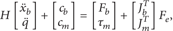
where
Separate (1), we can obtain the following equation:

Eliminate the base acceleration term

where H* = (H
q
-H2
T
H1−1H2) is the generalized inertial tensor,
According to the collision assumptions above, the Coriolis force, centrifugal force, and the velocity-dependent term can be neglected at the contact time. The integral during infinitesimal time interval δt is

where

As we know from the kinematics relationship (the initial momentum and angular momentum are assumed to be zero)
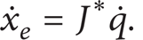
Hence, the instantaneously change in spatial velocity of the end-effector is

For a single-point contact, the impulsive force Φ is equal to the product of a scalar magnitude γ and its direction vector N, namely, Φ = Nγ. Substitute it into (7):

where D = J*H*−1J*T is called the Jacobian inertia.
A whole collision can be divided into two phases: the compression phase and the restitution phase. At the end of the compression phase, the velocity projection of end-effector is equal to that of contact point on the surface of the target along the collision direction N. We define ve1 and ve2 as the velocities of robot end-effector and the contact point of target just before contact, respectively; δve1 and δve2 are the corresponding changes. Thus, we can get the following equation:

Let -Nγ c represent the impulsive force applied on the robot end-effector during the compression phase, and the impulsive force applied on the target is Nγ c obviously. Then using the results of (8)

where D1 is the Jacobian inertia of manipulator and
Substitute (10) into (9), the impulsive force of the compression phase can be obtained:

Note that γ c >0 since it is necessary that N T (ve2-ve1)<0, for the collision objects have to contact first. Poisson model is employed during the collision; the impulsive force of the restitute phase is γ r = eγ c ; 0 ≤ e ≤ 1 is the coefficient of restitute. Therefore, the impulsive force of the whole collision phase is

3. The Optimization of Manipulator Configuration at the Contact Point
Non-minimum-norm solutions to (6) based on Jacobian pseudoinverse can be written in the general form [15]:

where J*† = J*T(J*J*T)−1 is the pseudoinverse of Jacobian matrix J*, (E-J*†J*) is called the null space, k is the gain coefficient, which can be a constant or a function, and φ is an arbitrary vector. By observing that null-space velocities produce a change in the configuration of the manipulator without affecting its velocity at the end-effector, it can be exploited to achieve additional goals; here, we mean the impulsive minimization.
From (12), we can see that the impulsive force is affected by the collision direction N, relative velocity ve12 = ve1-ve2, and the robot configuration D1. When N and ve12 are determined, the impulsive force can be minimized by optimizing its configuration. Assume g = N
T
(D2 + D1)N, the impulsive force is minimum when g is maximum. Set
In order to make the end-effector keep the correct capture pose when adjusting its configuration for minimizing the contact impulsive force, set

To make the initial joint angular velocities zero and run stably, we design the transition function k as follows:
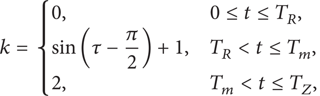
where
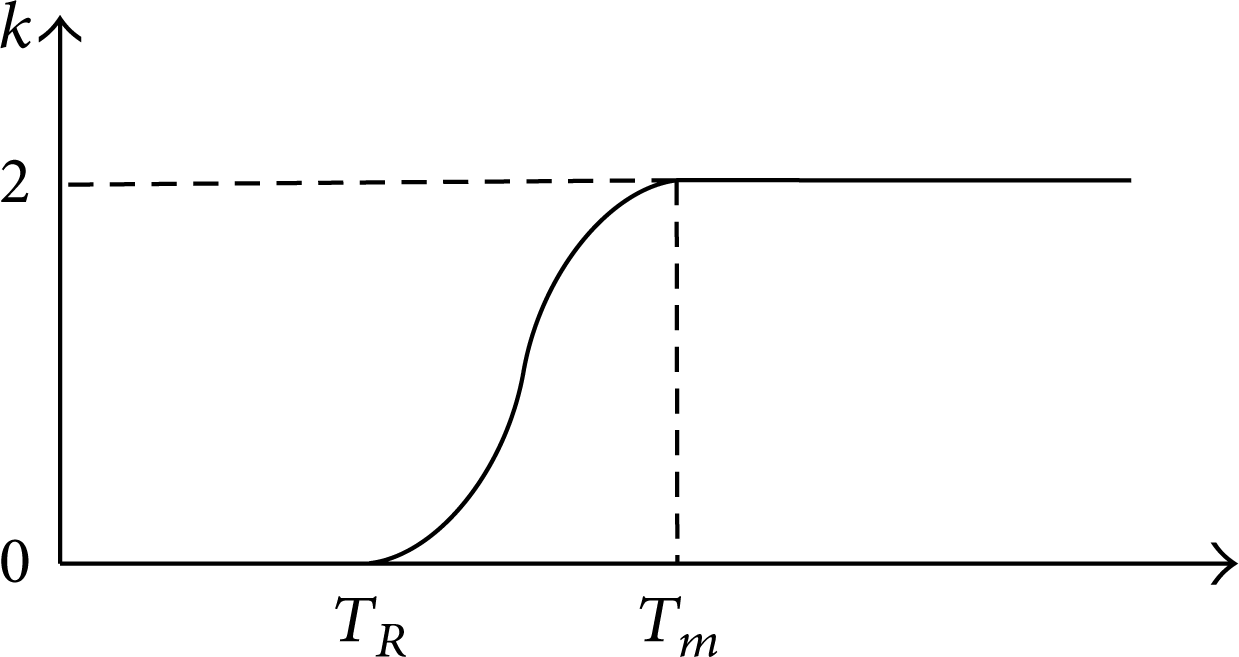
Curve of transition function k.
The specified steps for optimization are as follows.
Set the initial joint angles q0 and get the corresponding value of g, called g0; the initial joint angle velocities are set to be zero.
Optimize the joint angle velocities for maximizing g by (14); update the joint angles and the g value by
Compare the current gvalue gi with the previous one; if g i >gi–1, the optimization goes on, namely, loop to step 2.
Obtain the best configuration qd when g achieves its maximum.
The manipulator configuration will be optimized until the value of g achieves its maximum and remains unchanged. Through the method above, we can obtain the best configuration, which can satisfy the impulse force minimization (g maximum) and the capture pose of the end-effector correction.
4. The Precollision Trajectory Planning Based on PSO
We have obtained the best configuration at the contact point in Section 3; the following problem is how to plan the trajectory from the initial configuration to the desired configuration, and the correct capture pose of the end-effector needs to be achieved at the same time.
For a free-floating space manipulator, it exhibits nonholonomic characteristic due to the dynamic coupling between space manipulator and its base. Therefore, the planning and control of space manipulators have some additional problems beyond those on earth. We decide to employ the PSO algorithm to complete the precollision trajectory planning.
4.1. A Brief Review of PSO
Particle swarm optimization (PSO), a stochastic optimization method based on the simulation of the social behavior of bird flocks, was originally developed by Kennedy and Eberhart [16, 17]. It is similar to a genetic algorithm in that the system is initialized with a population of random solutions. It is unlike a genetic algorithm, however, in that each potential solution is also assigned a randomized velocity, and the potential solutions, called particles, are then “flown” through hyperspace. Each particle keeps track of its coordinates in hyperspace which are associated with the best solution it has achieved so far. The value is called pbest. Another “best” value, which is also tracked, is the overall best value, and its location, obtained so far by any particle in the population. This location is called gbest.
The particle flies in the search space at a certain speed and direction. According to its own flying experience and its companion's flying experience, it will change the velocity toward its pbest and gbest locations at each time step. Acceleration is weighted by a random term, with separate random numbers being generated for acceleration toward pbest and gbest. In a d-dimension space, the velocity and location of particle i are updated by the following equations:

where the acceleration constants c1 and c2 represent the weighting of the stochastic acceleration terms that pull each particle toward pbest and gbest positions. Low values allow particles to roam far from target regions before being tugged back, while high values result in abrupt movement toward, or past, target regions. c1 and c2 each equal to 2.0 is suitable for almost all applications.
4.2. The Solution Based on PSO
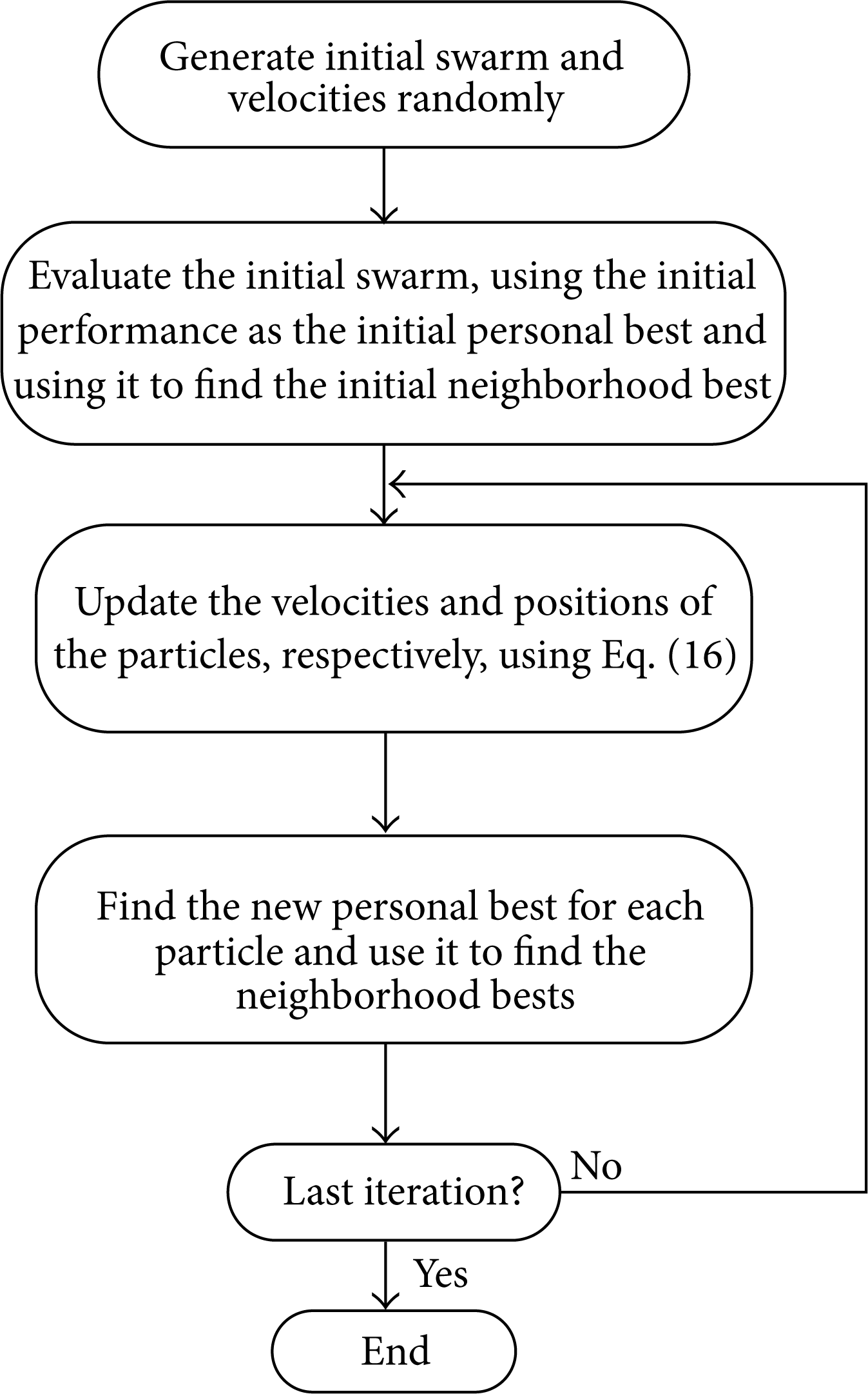
One of the reasons that PSO is attractive is that there are very few parameters to adjust. It has been used for space robot path planning in [18–20]. The process for implementing the PSO is as follows.
Initialize a population (array) of particles with random positions and velocities on d-dimension in the problem space.
For each particle, evaluate the desired optimization fitness function in d variables.
Compare particle's fitness evaluation with particle's pbest. If current value is better than pbest, then set pbest value equal to the current value and the pbest location equal to the current location in d-dimension space.
Compare fitness evaluation with the population's overall previous best. If current value is better than gbest, then reset gbest to the current particle's array index and value.
Change the velocity and position of the particle according to (16).
Loop to step 2 until a criterion is met, usually a sufficient good fitness or a maximum number of iterations (generations).
The flowchart of PSO is simply shown in Figure 3.
The flowchart of PSO.
Before optimization, the particles and objective function need to be determined. The joint variables are parameterized to be the particles, and the optimized results can be directly used to adjust the manipulator configuration. When the manipulator moves to the contact point, as mentioned above, it needs to be at the best configuration, and its end-effector needs to have the correct capture pose, so the objective function should contain all the information.
4.3. The Particles of PSO
As said above, the joint variables are parameterized to be the particles. First, the initial and final joint angles, angular velocities, and angular accelerations are expected to satisfy the following requirements:

where t0,t f are the initial and the final time and Θ0,Θ d are the initial and the desired final angles, respectively. Furthermore, the path planning solution has to satisfy the mechanical constraints of manipulator

where θ imax , θ imin are the lower and upper permitted angles of the ith joint. The polynomial functions are usually used to obtain smooth joint motion, and considering the joint angle limits, we parameterized the joint trajectory by a sinusoidal function, whose argument is a seventh-order polynomial

where ai7,ai6,…, ai0 are the coefficients of the polynomial, i = 1,2…, n is the ith joint,
The joint velocity and joint acceleration can be obtained by the derivate and second-derivate of (19). Considering (17), the following results are found:

where θi0, θ
id
are the initial and the desired angle of the ith joint. After parameterization, only two parameters (ai6,ai7) are included in each joint function. Thereby, let
4.4. The Objective Function of PSO
The best configuration of space manipulator has been achieved in (17); the correct capture pose can be realized through the following method.
The position of the end-effector is determined by velocity integral method, namely,
The attitude of the end-effector is represented by quaternion. The unit quaternion is a popular nonsingular four-parameter representation [21], which has several advantages over the conventional usage of direction cosines and Euler angles. First, a mechanical system that involves rotation between various coordinate systems does not degenerate for any orientation. Second, the computational cost of using the quaternion is less.
A quaternion

And it is constrained by η2 + q12 + q22 + q32 = 1.
According to [22, 23] and combining the kinematics knowledge, the variation rate of

where Jωe is the Jacobian matrix of angular velocity.
For two coordinate systems, their attitudes being represented by [η1,

When the two frames coincide

It's worth noting that δ
Suppose

Thus, the objective function of PSO can be designed as
where
5. Simulation Study
5.1. The Studied Robot System
The studied space manipulator is composed of the base and a 7-dof manipulator. Set a = k = 0.6 m, b = e = f = h = 0.5 m, c = d = 5 m. Its joint frames according to DH method are shown is Figure 4 and the relative parameters are listed in Tables 1 and 2.
DH parameters of space manipulator.

Dynamic parameters of space manipulator.


A 7-dof free-floating space manipulator.
The initial joint angle is set as Θ0 = g[−50°, −170°, 150°, −60°, 130°, 170°, 0°] and the final desired pose of the end-effector is [9.60 m, 0.00 m, 3.00 m, −1.00 rad, −0.50 rad, −2.00 rad]. Assume the target is a rigid sphere, whose mass is m
o
= 30kg and radius is R = 0.3 m. The inertial tensor is a diagonal matrix, whose elements are
5.2. The Configuration Optimization at the Contact Point
First, we can adopt any method to obtain a group of joint angles that are suitable for the capture pose. For example, we planned the end-effector of the manipulator to trace a straight line from the initial point to the desired point, and the velocity is planned by a symmetric trapezium curve with parabolic transition to make the acceleration change stably. Considering the limit of joint velocity, we assume that the whole planning time T A = 50 s, the acceleration time T s = 5 s, and the control cycle δT = 50 ms. And [−84.5°, −188.7°, 116.8°, −37.4°, 164.7°, 187.5°, −41.2°] is a suitable manipulator configuration at the contact time. The value of g function is 0.1468. Thereafter, regard this group of joint angles as the initial angles and use the method in Section 3 to optimize the configuration; the curve of g-value versus time is as shown in Figure 5.

g-value versus time during configuration optimization.
We can see that after about 80's, the value of g function approaches a constant value 0.1882, which is also the maximum value. And comparing with the g-value before optimization 0.1468, the amount of increase is 28.2%, which means that the configuration optimization minimizes the impulsive force greatly. In the process of optimization, the change of the end-effector pose is shown in Figures 6 and 7; the changes of joint angles and joint angle velocities are shown in Figures 8 and 9.
The position of the end-effector during the configuration optimization.

The attitude of the end-effector during the configuration optimization.

The changes of joint angles during the configuration optimization.

The changes of joint angle velocities during the configuration optimization.
From these figures, we know that in the process of configuration optimization, the end-effector stays at the correct capture pose. And the joint angle velocities all approach zero at the end time, which means that it has achieved the best configuration. This group of joint angles is [−92.6°, −119.8°, 100.3°, −22.5°, 196.6°, 211.3°, 28.8°].
5.3. The Precollision Trajectory Planning Based on PSO
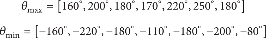
Set the limits of the joint angles as
c1 = c2 = 2.0, w1 = w2 = 50. The population size is 24. After 200 iterations we can get the optimal particle: 1.8e–08 × [0.22, 0.14, −2.56, 1.31, 1.64, 0.20, 5.41, −0.28, −4.40, 4.56, −4.30, −1.58, −5.60, 6.83]. And the value of objective function f is 0.0134, which means the convergence result is satisfactory. The convergence process is shown as Figure 10. Substitute the optimal particle into (19), we can obtain the changes of the joint angle and joint angle velocity in Figures 11 and 12.

The variation of the global best fitness evaluation.

The joint angles from initial point to the desired point.

The joint angle velocities from initial point to the desired point.
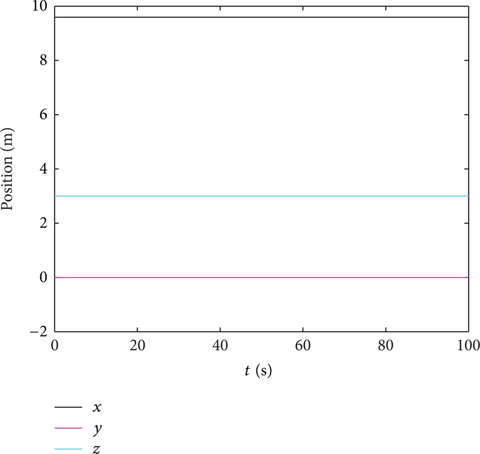
In light of the figures, it can be seen that both the joint angle curves and the joint angle velocity curves are smooth and steady, which means this method can be applied to actual operation. And the final pose of the end-effector is [9.59 m, −0.01 m, 3.00 m, −1.00 rad, −0.49 rad, −2.00 rad]; the deviations are acceptable. As for the effect for the impulsive force minimization, through comparison of g value between the before and after optimization in Section 5.2, it proves that the proposed method minimizes the impulsive force greatly.
6. Conclusions
The on-orbit capture operation of free-floating objects by a space robot has become an important mission in recent years. Through the analysis of task characteristics, a scheme for precollision trajectory planning of redundant space manipulator is proposed in this paper. This scheme can obtain the minimized collision impulsive force and the correct capture pose at the same time. In the simulation experiment, the 28.2% increase of g verifies the effectiveness of minimizing the impulsive force and the joint angles; joint angular velocities as well as the the capture pose obtained by the PSO algorithm demonstrate the feasibility in actual application of space manipulator.
Conflict of Interests
The authors declare that there is no conflict of interests regarding the publication of this paper.
Footnotes
Acknowledgments
This project is supported by the National Natural Science Foundation of China (61175080), the National Key Basic Research Program of China (2013CB733000), the Specialized Research Fund for the Doctoral Program of Higher Education (20120005120004), and the Fundamental Research Funds for the Central Universities (2013PTB-00-01).