A Location Estimation Algorithm Based on RSSI Vector Similarity Degree

Abstract

We present a detailed study on the RSS-based location techniques in wireless sensor networks (WSN). There are two aspects in this paper. On the one hand, the accurate RSSI received from nodes is the premise of accurate location. Firstly, the distribution trend of RSSI is analyzed in this experiment and determined the loss model of signal propagation by processing experimental data. Secondly, in order to determine the distance between receiving nodes and sending nodes, Gaussian fitting is used to process specific RSSI at different distance. Moreover, the piecewise linear interpolation is introduced to calculate the distance of any RSSI. On the other hand, firstly, the RSSI vector similarity degree (R-VSD) is used to choose anchor nodes. Secondly, we designed a new localization algorithm which is based on the quadrilateral location unit by using more accurate RSSI and range. Particularly, there are two localization mechanisms in our study. In addition, the generalized inverse is introduced to solve the coordinates of nodes. At last, location error of the new algorithm is about 17.6% by simulation experiment.

1. Introduction

Localization is certainly needed for robots to efficiently carry out given tasks such as cleaning, serving, and guiding. It is a challenging research topic in mobile robot which has received much attention [1]. Moving around without location for robots is the same as walking with closed eyes for people [2]. They do not know where they are and which direction they should move to. Under this background, reliable and efficient localization is still a critical issue for mobile robots. Research on localizing mobile robots has come to prominence in wireless sensor network over the last years [3].

To a large extent, WSN has changed the current situation that people get information by the traditional way, such as their sense of touch, sight, and smell. WSN has become a new formula of technology to get data. Wherever in the field of national security or national economy building, WSN has been applied widely [4]. In a variety of applications in WSN, only if the location information of the node itself is combined with the information which is captured and collected from sensor nodes “the location of the incident” can be illustrated accurately and the region of target monitoring is reflected truly. Obviously, the location information of the node is the premise of sensor nodes that are perceived and collected data. It is imprecise and lacking practical significance that there is only perception data of nodes and there is not the perception of location information which signed the source of perception data [5]. Therefore, it is important to locate the node in WSN, so the location technology also is becoming an essential function and a critical supporting technology in WSN [6]. In terms of the collection of network data and event monitoring, the location information of nodes is important. In the field of remote sensing, it is significant to track and monitor. It is contributed to compare composited route and optimize communication task and improve composited routing table [7]. Some domestic scholars also research on deep discussions of localization in WSN [8, 9]. Unknown nodes and anchor nodes are two important parts of location system. In addition, in terms of choosing anchor nodes, some researchers pay attention to research on RSSI-similarity degree [10].

There are two existing formulas of methods of node localization in WSN by measuring distance or angle information between nodes in the location process and not measuring information: the method is based on range location (Range-based) and without range location (Range-free) [11]; the information of range or angle between communication nodes is obtained; it is the premise of the former method to locate nodes; the latter method is not needed to measure range information between nodes directly; it is estimated coordinates of nodes just by getting information of communication hops between nodes or network connectivity. There are common ranging methods as follows: TOA ranging method [9, 11], TDOA ranging method  [11], AOA ranging  [12], and RSSI ranging method [13].

Range is the premise of location; precise range is the assurance of accurate location. Only a certain number of reference nodes (anchor nodes) are combined with effective localization algorithm if they ensured feasible location task, lots of equipment is included in the process; they are arranged before and are able to communicate. At the same time, in the place of receiving nodes, information of signal strength and angle between nodes is needed to measure and convert it into distance information. With the help of geometric or mathematical relationships we can carry out the location task after achieving information of distance or orientation between nodes. In typical location algorithms, the method of Range-based mainly included trilateral location and triangulation location and maximum likelihood location; Range-free mainly included centroid location, convex programming location, and DV-Hop location method.

The principle of Hop count [12] ranging method is based on hop counts between anchor nodes and unknown node and the product of distance of mean hop in the network to determine their distance. Information of hop count is obtained as follows: anchor nodes send a packet which included lots of information such as its location information to the network, if receiving nodes received the packet, it will add one hop to itself and retransmission, until the unknown node receives this packet; at this time, the minimum hop (the shortest path) is regarded as the hop count between anchor nodes and the unknown node. This range method requires the uniform distribution of nodes in the network; it can ensure that the distance of mean hop in the network better reflected the layout of nodes and achieved higher ranging precision.

The coordinate of the unknown node is estimated by the trilateral location method; it has got good effect [14].

In [15], the value of nodes localization is achieved by the steepest descent algorithm which is a modified algorithm of maximum likelihood estimation method; moreover, the location accuracy and smaller computational cost can be obtained from the steepest descent algorithm which has obvious effect. In [16], the maximum likelihood estimation and the Kalman filtering are composited; it has a double effect on node prelocation and tracking, and it also has higher location accuracy.

The location principle of centroid localization is as follows: the unknown node sends broadcast messages to the network for determining its location information; after anchor nodes received broadcast messages, they sent response of information of its own location to the unknown node; the center of mass in this graphic is regarded as the estimation coordinate of the unknown node [17, 18], which is formed by anchor nodes.

In [19], Approximate Point In triangulation Test (APIT) is mentioned. It is a concrete application of centroid localization method; the location principle is as follows: there are any three anchor nodes that composed one triangle; there is a collection formed by all triangles which included the unknown node; the coordinate of the unknown node is determined by determining the center of mass of graphic which is composed of all triangles of the collection.

Centroid algorithm is the most popular algorithm in many location methods in WSN, because the easy operation and the characteristics of few errors are included in the algorithm. Yedavalli and Krishnamachari has put forward sequence of location algorithm [20] (SBL, Sequence-based Localization); Liu et al. has put forward a new SBL algorithm; it combined SBL with three orthocenter algorithm [21]; it is a concrete instance of centroid localization method; it achieved good localization accuracy, but it is needed to improve on boundary node location or ideal environment.

The location principle of convex programming location method [22] (convex optimization) is that the whole network is regarded as a model of convex collection by using the network connectivity; it is through the way of bound combination and plans to determine the possible region within the unknown node and estimate coordinates.

In [23], researchers have analyzed location methods of DV-Hop and DV-distance; the experimental result has shown that the location accuracy can achieve 20% when the network connectivity is 9 and the proportion of anchor nodes is 10%, but the location accuracy is declining evidently along with the increasing range error. Zhang and Wu have put forward a modified location algorithm [24] which is based on the estimation of mean hop distance and location correction; it has solved the situation that the distance of mean hop cannot reflect the real distance, which is estimated by the single anchor node in the network. The result of experiment has shown that mean error of the modified algorithm is reduced about 8.8497% and 14.457%; it has achieved better location accuracy.

In this paper, a novel location algorithm based on RSSI vector similarity degree is presented and a location system is designed, which is applied to locate sensor nodes indoor. Our proposed contributions are as follows.

• (1)

The Gaussian fitting has optimized the value of RSSI at different distance.

(2)

The linear interpolation is used to decrease the calculation of RSSI; it is according to the relation between different RSSI and distance.

(3)

The vector similar degree is helpful in choosing anchor nodes.

(4)

The generalized inverse is solved to estimate the coordinate of unknown node by equations.

(5)

The location system is able to work well indoor when the mobile node is dynamic.

2. Ranging Method of RSSI-Based

Received signal strength indicator (RSSI) indicated the energy loss in the process of signal transmission; the RSSI value is associated with the size of signal attenuation. In the process of signal transmission, the smaller the RSSI value the less the attenuation. Usually, the RSSI ranging [25] is based on the experience model or theory model. The RSSI ranging of model-based experience has shown that an offline database is built between few RSSI values of nodes which are known location information and their distance of signal propagation; in the process of nodes location, the stored data in the database is constantly compared to implement nodes location. The RSSI ranging model-based theory implemented nodes localization by determining the environmental parameters in the loss model of signal propagation and plugging the RSSI value which is received from receiving nodes into the model, so as to estimate distance between nodes. There is a key of former method; lots of measuring work of off-line in the region is required; in addition, the location accuracy is limited by the number of nodes and measuring workload. The core of the latter method lied in researching on critical parameters of the model detail by the accurate measuring of RSSI value; hardware conditions and actual environment can be better reflected; in addition, location accuracy and improved location performance can be enhanced.

Common methods of RSSI ranging are as follows, which are based on the theory model: the path loss model of free space propagation [26] and the block model of logarithmic normal  [26] (Shadowing model), and so forth.

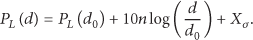
The path loss model of free space propagation is an ideal transmission case, it is known that there is an infinite vacuum around antenna, the signal transmission energy is only related to transmission distance, there is a linear relationship between the signal transmission energy and transmission distance, this model has no effect on obstacles and scattered reflection, and so forth. The path loss model [26] is as follows:

$$\begin{array}{cc}& \text{Loss}=\mathrm{32.44}+\mathrm{10}n\log \left(d\right)+\mathrm{10}n\log \left(f\right).\end{array}$$

(1)

In this formula, loss indicated the path loss of signal energy, d indicated the signal transmission distance (m), f indicated the wireless signal frequency (MHz), and n indicated the path attenuation factor in the actual environment.

However, the application environment of wireless sensor signal is not in a free space, but in the actual environment such as industrial sites or indoor buildings; it needs to consider shade and absorbance by obstacles and the interference of scattered reflection, and so forth. The attenuation characteristic of channels in the long distance is following the lognormal distribution; it is commonly used by the block model of logarithmic normal; the path loss model is as follows:

$$\begin{array}{cc}& P_L\left(d\right)=P_L\left(d_{\mathrm{0}}\right)+\mathrm{10}n\log \left(\frac{d}{d_{\mathrm{0}}}\right)+X_{\sigma }.\end{array}$$

(2)

In this formula, $P_L(d)$ indicated the path loss of receiving sign when the measuring distance is $d\hspace{0.17em}(\text{m})$ , it indicated the absolute power value, and it is in $\text{dBm}$ ; $P_L(d_{\mathrm{0}})$ indicated the path loss of receiving sign when the reference distance is $d_{\mathrm{0}}$ ; n indicated the path loss index in a specific environment; it indicated the speed of the path loss, which is increased along with increasing distance; $X_{\sigma }$ is in dB; it is a cover factor when the range of standard deviation σ is 4~10 and the mean value is 0; the larger the σ, the greater the uncertainty of the model. The signal strength of receiving nodes is as follows:

$$\begin{array}{cc}& \text{RSSI}=P_t-P_L\left(d\right).\end{array}$$

(3)

In this formula, $P_t$ indicated the signal transmission power, $P_L(d)$ indicated the path loss when the distance is d, and they are both in $\text{dBm}$ . A indicated the signal strength which is received from reference nodes at the distance $d_{\mathrm{0}}$ ; A is as follows:

$$\begin{array}{cc}& A=P_t-P_L\left(d\right).\end{array}$$

(4)

The path loss model is as follows, which is measured at the real distance $d\hspace{0.17em}(\text{m})$ :

$$\begin{array}{cc}& P\left(d\right)=P\left(d_{\mathrm{0}}\right)-\mathrm{10}n\log \left(\frac{d}{d_{\mathrm{0}}}\right)-X_{\sigma }.\end{array}$$

(5)

In this formula, $P(d)$ indicated the received signal strength when the measured real distance is $d\hspace{0.17em}(\text{m})$ . $P(d_{\mathrm{0}})$ indicated received signal strength when the reference distance is $d_{\mathrm{0}}$ , $X_{\sigma }~N(\mathrm{0},{\sigma }^{\mathbf{2}}\mathbf{)}$ .

We take the reference distance $d_{\mathrm{0}}=\mathrm{1}\hspace{0.17em}\text{m}$ ; it can be obtained from formula (3) and formula (5).

$$\begin{array}{cc}& \text{RSSI}=A-\mathrm{10}n\log \left(\frac{d}{d_{\mathrm{0}}}\right)-X_{\sigma }.\end{array}$$

(6)

$\overline{\text{RSSI}}$ is regarded as RSSI value of multiple times of measurement

$$\begin{array}{cc}& \overline{\text{RSSI}}=A-\mathrm{10}n\log \left(d\right).\end{array}$$

(7)

d is regarded as the undetermined distance

$$\begin{array}{cc}& d=\mathrm{1}{\mathrm{0}}^{\left(A-\text{RSSI}\right)/\mathrm{10}n}.\end{array}$$

(8)

The Shadowing model is chosen to indicate the power attenuation in the process of the wireless signal transmission; due to various obstacles and interference factors, there are kinds of the wireless signal propagation environment; it can be reflected the real measurement environment by determining related environmental parameters in the model.

2.1. RSSI Ranging Method Based on Gaussian Fitting

As shown in Shadowing model, there is a corresponding relationship between wireless signal propagation loss and transmission distance in the actual test environment. It means that according to the received information of signal strength the distance between sending nodes and receiving nodes can be obtained. However, the conclusion of experiment cannot rely on one time of measurement task, but on the basis of a large number of test data. So, in terms of the same node and the same distance, received signal strengths are taking many times of measures. On the basis of measurement, the distribution trend of RSSI in the test environment is analyzed and interference data and error data are eliminated; the most representative signal strength value at specific distance is obtained; signal strength is regarded as the basis of distance estimation at this place.

2.1.1. Experimental Environment

The location system is included the hardware platform and software platform. Hardware platform included anchor nodes and unknown node, gateway control equipment. The measurement is worked on the perception platform of SensorRF107H2 0, the sensing platform is designed by the wireless gateway which owned the core of high-performance microcontroller and in 32-bit ARM, and it included advanced designing tools of software and hardware such as online emulators when users develop, debug, and test software. Anchor nodes and unknown node are composed of modules of CC2530 of the system of ZigBee which is included TI.

2.1.2. Acquisition of RSSI Data

Signal strength indicator (RSSI) is read from the register RSSI_VAI in the data packets which are received from sensor receiving nodes, a sensor node is set and regarded as a receiving device at intervals of 1 m, RSSI data is measured more than 400 times at every place, and each sensor node is received and recorded its signal strength value. Receiving nodes only can receive few signal strength values beyond 25 m; parts of signal value are not detected, because the RSSI value of characterization signal attenuation is included in data packets, so it is meaningless to keep measuring. In this paper, the range of RSSI ranging is kept 0~25 m. For example, the distance between sending node and receiving node is taken 5 m and 10 m, respectively, we have made statistics for collecting RSSI value and chosen more than 400 times of measurement to be a sample and got the characteristics picture of RSSI, and they are as in Figures 1 and 2.

Figure 1

RSSI experimental data of node at d = 5 m.

Figure 2

RSSI experimental data of node at d = 10 m.

Figures 1 and 2 can be seen, with the passage of time; although RSSI generally presented obvious nonstationary characteristics, the RSSI value in certain distance are always fluctuated up and down between the constant real RSSI value, the closer distance from emission node, and the frequenter change of measurement value; on the contrary, the farther the distance from emission node, the gentler the change.

2.1.3. Shadowing Model

In order to exactly describe the actual measurement environment and ensure the accuracy of RSSI ranging, the parameters of signal propagation model are needed to define. A indicated the received signal strength value when the reference distance is $d_{\mathrm{0}}=\mathrm{1}\hspace{0.17em}\text{m}$ and n indicated the path loss index.

The determination of parameter A is as follows.

$A=P(d_{\mathrm{0}})$ , the radio frequency parameter A indicating the received absolute value of mean energy, which is received from the projection node when distance is 1 m; it is in $\text{dBm}$ . When the distance is $\mathrm{1}\hspace{0.17em}\text{m}$ , 500 groups of data are continuously measured; finally, there is a result that $A=\mathrm{117}$ .

The determination of parameter n is as follows.

Environment factor n indicated, along with the increasing distance, the speed of signal loss in the process of actual transmission. They are satisfied with the following relationship:

$$\begin{array}{cc}& n=\frac{A-\overline{\text{RSSI}}}{\mathrm{10}*\log \left(d\right)},\end{array}$$

(9)

where n is obtained by generating into more than 3000 groups of data in the range of $\mathrm{2}~\mathrm{10}\hspace{0.17em}\text{m}$ ; it is as in Table 1.

Table 1

The value of n.

	Distance
	2 m	3 m	4 m	5 m	6 m	7 m	8 m	9 m	10 m
n	5.982	5.904	5.421	7.908	6.670	10.820	6.496	7.507	6.070

The mean value n can be obtained as follows:

$$\begin{array}{cc}& n={{\displaystyle \sum }}_{i=\mathrm{2}}^{\mathrm{10}}{n}_i=\mathrm{6.9861}.\end{array}$$

(10)

The Shadowing transmission model can be obtained by combining with parameter A and parameter n; it is as follows:

$$\begin{array}{cc}& P\left(d\right)=\mathrm{117}-\mathrm{10}*\mathrm{6.9861}*\log \left(\frac{d}{d_{\mathrm{0}}}\right)-X_{\sigma }.\end{array}$$

(11)

2.1.4. The Distribution Trend of RSSI and Gaussian Fitting

In order to analyze the distribution trend of RSSI, many groups of RSSI data are integrated and analyzed and drew four groups of probability density curves when RSSI is, respectively, 117 DBM, 89 DBM, 61 DBM, and 25 DBM; the results are as in Figures 3, 4, 5, and 6.

Figure 3

First group of RSSI probability density.

Figure 4

Second group of RSSI probability density.

Figure 5

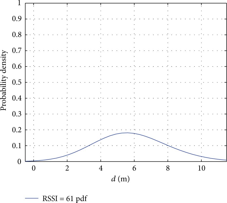
Third group of RSSI probability density.

Figure 6

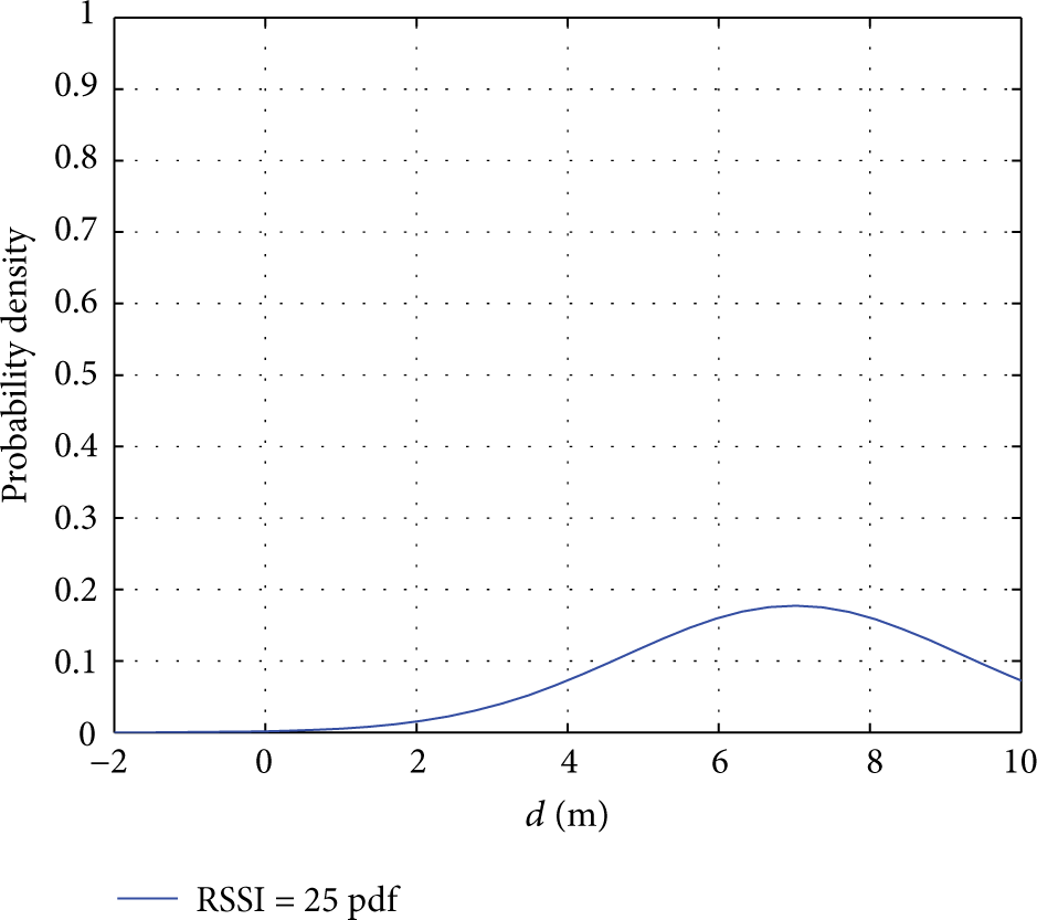
Fourth group of RSSI probability density.

It can be seen from Figures 3, 4, 5, and 6 of RSSI probability density that the distribution of RSSI value of the real measurement presented a probability distribution; there are some characteristics are as follows.

Concentration. The peak of the curve (the mean location) is located in the central.

Basic Symmetry. Two sides of curves are basic symmetry and ends of the curve are closed to horizontal axis. The centre of curves is based on mean value.

Volatility. The trends of two sides of curves are declined gradually at the place of mean value.

Some scholars also research on the kind of distribution of RSSI [27–29]; they think RSSI value approximately followed normal distributions as a whole. According to the experimental data and probability density in this paper, it can be seen that there is a similarity between actual measured probability density of RSSI and normal distribution [30]. So Gaussian fitting is used to fit RSSI value in experiment and probability error and invalid data are eliminated, the peak value of probability is found, the estimating distance is extracted, which is closer to the real distance, and the process is prived an experiment basis to get accurate location.

If RSSI data is closed to normal distribution, the peak of normal distribution will be the place of the greatest probability density, and the RSSI value is most likely the corresponding distance. So the Gaussian fitting [31] is used to fit the original RSSI data by looking for the peak of probability density; it is aimed at reducing the interference that small probability events have an effect on the overall measurement process. In order to improve the precision of RSSI ranging, the least square [32] is used to fit curves of probability density of RSSI.

$(\text{RSS}{\text{I}}_i,f_i)$ is described in a two-dimensional coordinate system; $\text{RSS}{\text{I}}_i$ indicated the ith value of signal strength; $f_i$ indicated the peak value of probability density, which is correspondent to $\text{RSS}{\text{I}}_i$ ; there is a relationship as follows:

$$\begin{array}{cc}& f=g\left(\text{RSSI},a_{\mathrm{1}},a_{\mathrm{2}},\dots ,a_N\right).\end{array}$$

(12)

In this formula, $a_{\mathrm{1}},a_{\mathrm{2}},\dots ,a_N$ indicated N pending constant.

There is an assumed fitting function between $\text{RSS}{\text{I}}_i$ and $f_i$ as follows:

$$\begin{array}{cc}& \widehat{f}=g\left(\text{RSSI},{\widehat{a}}_{\mathrm{1}},{\widehat{a}}_{\mathrm{2}},\dots ,{\widehat{a}}_N\right).\end{array}$$

(13)

In this formula, ${\widehat{a}}_{\mathrm{1}},{\widehat{a}}_{\mathrm{2}},\dots ,{\widehat{a}}_N$ indicated the optimal estimating value which is correspondent to constants of original function. If fitting points are falling on the curve of the original function, there will be a relationship as follows:

$$\begin{array}{cc}& f_i=g\left(\text{RSS}{\text{I}}_i,a_{\mathrm{1}},a_{\mathrm{2}},\dots ,a_N\right)\hspace{1em}\left(i=\mathrm{1,2},\mathrm{3},\dots ,m\right).\end{array}$$

(14)

However, under normal circumstances, the original function and the fitting function do not have to be same, there is a residual relationship as follows:

$$\begin{array}{cc}& e_i=f_i-{\widehat{f}}_i\hspace{1em}\left(i=\mathrm{1,2.3},\dots ,m\right).\end{array}$$

(15)

The smaller the residual $e_i$ the smaller the difference between fitting function and original function; $f_i$ can be better reflecting the distribution trend of $\text{RSS}{\text{I}}_i$ at different distance. If all errors are following normal distribution, the probability $P(e_{\mathrm{1}},e_{\mathrm{2}},\dots ,e_m)$ will be changed; there is a formula as follows:

$$\begin{array}{cc}& P\left(e_{\mathrm{1}},e_{\mathrm{2}},\dots ,e_m\right)=\frac{\mathrm{1}}{\sigma \sqrt{\mathrm{2}\pi }}\exp \left[-{{\displaystyle \sum }}_{i=\mathrm{1}}^m\frac{{\left(f_i-{\widehat{f}}_i\right)}^{\mathrm{2}}}{\mathrm{2}{\sigma }^{\mathrm{2}}}\right].\end{array}$$

(16)

The fitting curve will be the best fitting form of the original curve, if $P(e_{\mathrm{1}},e_{\mathrm{2}},\dots ,e_m)$ got the peak of normal distribution. At the same time, the sum of squares of fitting residual is minimal; there is a formula as follows:

$$\begin{array}{cc}& S={{\displaystyle \sum }}_{i=\mathrm{1}}^m{\left(f_i-{\widehat{f}}_i\right)}^{\mathrm{2}}={{\displaystyle \sum }}_{i=\mathrm{1}}^m{e_i}^{\mathrm{2}}.\end{array}$$

(17)

Formula (18) can be described as

$$\begin{array}{cc}& S={{\displaystyle \sum }}_{i=\mathrm{1}}^m{\left[f_i-g\left(\text{RSS}{\text{I}}_i,{\widehat{a}}_{\mathrm{1}},{\widehat{a}}_{\mathrm{2}},\dots ,{\widehat{a}}_N\right)\right]}^{\mathrm{2}}.\end{array}$$

(18)

Obviously, there are relationships as follows:

$$\begin{array}{cc}& \frac{\partial S}{\partial a_{\mathrm{1}}}=\mathrm{0},\frac{\partial S}{\partial a_{\mathrm{2}}}=\mathrm{0},\dots ,\frac{\partial S}{\partial a_N}=\mathrm{0},\\ {{\displaystyle \sum }}_{i=\mathrm{1}}^m\left[f_i-g\left(\text{RSS}{\text{I}}_i,{\widehat{a}}_{\mathrm{1}},{\widehat{a}}_{\mathrm{2}},\dots ,{\widehat{a}}_N\right)\right]\left(\frac{\partial f}{\partial a_{\mathrm{1}}}\right)=\mathrm{0},\\ {{\displaystyle \sum }}_{i=\mathrm{1}}^m\left[f_i-g\left(\text{RSS}{\text{I}}_i,{\widehat{a}}_{\mathrm{1}},{\widehat{a}}_{\mathrm{2}},\dots ,{\widehat{a}}_N\right)\right]\left(\frac{\partial f}{\partial a_{\mathrm{2}}}\right)=\mathrm{0},\\ ⋮\\ {{\displaystyle \sum }}_{i=\mathrm{1}}^m\left[f_i-g\left(\text{RSS}{\text{I}}_i,{\widehat{a}}_{\mathrm{1}},{\widehat{a}}_{\mathrm{2}},\dots ,{\widehat{a}}_N\right)\right]\left(\frac{\partial f}{\partial a_N}\right)=\mathrm{0},\end{array}$$

(19)

where $a_{\mathrm{1}},a_{\mathrm{2}},\dots ,a_N$ is determined by solving the above equation; at the same time, the least square solutions of the equation is obtained.

Figure 7 has shown the probability density of fitting when RSSI = 117 DBM. Since then, the RSSI value at the highest peak of curve is regarded as the signal strength value (distance 1 m). Similarly, in terms of any RSSI value, the distance is regarded as the basis of distance estimation, which is correspondent to the peak of probability density.

Figure 7

The gauss curve fitting when RSSI = 117.

The Gaussian fitting function protoformula is as follows:

$$\begin{array}{cc}& f\left(x\right)=a*e\frac{-\mathrm{2}{\left(x-\mu \right)}^{\mathrm{2}}}{{\omega }^{\mathrm{2}}},\\ \mu =\frac{{\sum }_{i=\mathrm{1}}^n\text{RSS}{\text{I}}_i}{n},\hspace{1em}\hspace{1em}\omega =\sqrt{\frac{{\sum }_{i=\mathrm{1}}^n{\left(\text{RSS}{\text{I}}_i-\mu \right)}^{\mathrm{2}}}{n-\mathrm{1}}}.\end{array}$$

(20)

The fitting probability density curve of RSSI = 117 DBM is as follows:

$$\begin{array}{cc}& f\left(x\right)=\mathrm{0.4643}*e^{{\left(\left(x-\mathrm{117}\right)/\mathrm{1.214}\right)}^{\mathrm{2}}}.\end{array}$$

(21)

Figure 7 has shown that the maximum value of the original probability density is $\text{RSSI}=\mathrm{117}\hspace{0.17em}\text{dBm}$ , but the maximum probability value of fitting is $\mu =\mathrm{117}\hspace{0.17em}\text{dBm}$ . There is the same effect between fitting and original.

2.2. Ranging Method Based on Interpolation

400 groups of RSSI data are taken at intervals of permanent distance; in Figure 8, the blue line is the real measurement value of RSSI in different distance; it can be seen that, with the increasing distance, different distance of RSSI overall has shown the trend of exponential attenuation, but there is a certain fluctuation which is influenced on interference factors around. The green line is the fitting value of RSSI in different distance.

Figure 8

The trend of curves of RSSI value between experiment and fitting.

Due to the fact that the trend of RSSI value is in accord with the distribution characteristics of indexes, the least squares are also used to fit the indexes function between the relation of RSSI-d, 0.0001237 and 128.2 are presented in this formula when the range of RSSI value is taken from 117 DBM to RSSI = 61 DBM, and there is a formula of fitting curve as follows:

$$\begin{array}{cc}& y\left(x\right)=\mathrm{0.0001237}{e}^{\mathrm{0.4185}*x}+\mathrm{128.2}{e}^{-\mathrm{0.1224}*x}.\end{array}$$

(22)

Figure 8 has shown the relationship between the experimental RSSI-d value and the fitting curve, respectively, the blue line indicated RSSI curve and the green line indicated fitting curve; in the graph, it can be seen that there is a deviation between fitting result and experimental RSSI-d at individual distance, but on the whole, it tended the exponential decay. Due to the fact that the obvious transmission signal is quickly attenuated at close distance, there is a slow attenuation and increasing error when the distance is farther. From the experimental figure it can be also seen that there is a better effect when the fitting curve is within 6 m and the trend of fitting error is smaller; along with the increasing distance, the fitting effect has shown a certain deviation and the fitting error is increased. So there is a linear relationship of RSSI value between adjacent distances which is less than 10 m, the not-measured RSSI value can be obtained by using the interpolation [33].

It is known that the real RSSI value is close to Gaussian distribution at different distance by analyzing the above section; the place of larger distribution density of RSSI is most likely to be the distance between receiving nodes and projection nodes. As shown in Figure 9, the corresponding RSSI value is measured at intervals of 1 m and the distribution of probability density is analyzed. The probability density curves when RSSI = 117 DBM and RSSI = 61 DBM are drawn, respectively, in the diagram. But it is uncertain that the not-measured RSSI value is at the distance of 1.5 m and 2.5 m; similarly, in terms of a given RSSI value, the distance between sending nodes and receiving nodes is uncertain. To this end, the interpolation mode is built according to the measured probability distribution of RSSI value; the distance between nodes is estimated according to the received RSSI value.

Figure 9

The curve of probability density when RSSI = 117 and RSSI = 61 DBM.

The Gaussian fitting is used to fit the probability distribution of RSSI. There is a fitting function as follows:

$$\begin{array}{cc}& f\left(\text{RSS}{\text{I}}_i\right)=f_{\mathrm{0}}+a*e\frac{-\mathrm{2}{\left(\text{RSS}{\text{I}}_i-\overline{\text{RSSI}}\right)}^{\mathrm{2}}}{{\sigma }^{\mathrm{2}}},\\ \overline{\text{RSSI}}=\frac{{\sum }_{i=\mathrm{1}}^n\text{RSS}{\text{I}}_i}{n},\hspace{1em}\hspace{1em}\sigma =\sqrt{\frac{{\sum }_{i=\mathrm{1}}^n{\left(\text{RSS}{\text{I}}_i-\mu \right)}^{\mathrm{2}}}{n-\mathrm{1}}}.\end{array}$$

(23)

Parameters $f_{\mathrm{0}}$ and a can be determined by two groups of specific RSSI value, such as RSSI = 117 DBM and RSSI = 61 DBM. The peak of probability density of RSSI is searched at each distance; the distance is regarded as the estimation distance between receiving nodes and sending nodes, which is corresponded to the peak. Along with the increasing distance between nodes, the RSSI value between nodes is decreased, so there is a linear relation between the peak of probability density and distance as follows:

$$\begin{array}{cc}& d=f{\left(\text{RSS}{\text{I}}_i\right)}_{\max }*k+b.\end{array}$$

(24)

Along with the changed distance, parameters k and b indicated the changed tendency of the probability density; they can be obtained by generating data. The model of RSSI-d is shown as follows [34]:

$$\begin{array}{cc}& d=\max \left(f_{\mathrm{0}}+a*e\frac{-\mathrm{2}{\left(\text{RSS}{\text{I}}_i-\overline{\text{RSSI}}\right)}^{\mathrm{2}}}{{\sigma }^{\mathrm{2}}}\right)*k+b.\end{array}$$

(25)

As shown in Figure 10, $f_{1\max }$ and $f_{2\max }$ indicated functions of RSSI₁ and RSSI₂, respectively, so, in terms of for all $\text{RSS}{\text{I}}_i\in (\text{RSS}{\text{I}}_{\mathrm{1}},\text{RSS}{\text{I}}_{\mathrm{2}})$ , if the corresponding equation $f_{i\max }\in (f_{\mathrm{1}\max },f_{\mathrm{2}\max })$ is needed to be obtained, there is a relationship as follows:

$$\begin{array}{cc}& \beta =\frac{f_{i\max }-f_{\mathrm{1}\max }}{\text{RSS}{\text{I}}_i-\text{RSS}{\text{I}}_{\mathrm{1}}}=\frac{f_{\mathrm{2}\max }-f_{i\max }}{\text{RSS}{\text{I}}_{\mathrm{2}}-\text{RSS}{\text{I}}_i}.\end{array}$$

(26)

In formula (26), β indicated the interpolation coefficient, in terms of any couples of RSSI according to the linear rule; their coefficient β is the same value. So, there is an equation between different couples of RSSI. If $\beta >\mathrm{1}$ , it is indicated that the $\text{RSS}{\text{I}}_i$ is in the range of $\text{RSS}{\text{I}}_{\mathrm{1}}$ and $\text{RSS}{\text{I}}_{\mathrm{2}}$ , so the extrapolation can be used; on the contrary, if $\beta <\mathrm{1}$ , the interpolation can be used.

Figure 10

The linear interpolation.

If it is known that $\text{RSS}{\text{I}}_i$ , the corresponding normal peak $f_{i\max }$ , is calculated by $f_{i\max }=(\mathrm{1}-\beta )*f_{\mathrm{1}\max }+\beta *f_{\mathrm{2}\max }$ ; according to (26), the distance $d_i$ which is most likely correspondent to RSSI can be obtained.

In this experiment, in the range of 0~25 m, all mean values of signal strength and standard deviation are indicated as follows:

$$\begin{array}{cc}& \overline{\text{RSSI}}={{\displaystyle \sum }}_{i=\mathrm{1}}^{\mathrm{25}}\text{RSS}{\text{I}}_i=\mathrm{64.8864}\hspace{0.17em}\text{dBm},\\ \sigma =\sqrt{\frac{{\sum }_{i=\mathrm{1}}^n{\left(\text{RSS}{\text{I}}_i-\overline{\text{RSSI}}\right)}^{\mathrm{2}}}{n-\mathrm{1}}}=\mathrm{32.4792},\\ f{\left(\text{RSSI}=\mathrm{117}\right)}_{\max }=\mathrm{0.3989},\hspace{1em}\hspace{1em}f{\left(\text{RSSI}=\mathrm{61}\right)}_{\max }=\mathrm{0.1816},\end{array}$$

(27)

and indicated the probability density when RSSI = 117 and RSSI = 61 by generating the related data into formula (23), and the interpolation model of RSSI-d is built as follows. When the distance is 1 m and RSSI is 117 DBM, $a=-0.3534$ and $b=0.401$ are obtained from formula (25), and the equation is as follows:

$$\begin{array}{cc}& d=\mathrm{0.401}+\left(-\mathrm{0.3534}\right)*e^{-\mathrm{2}{\left(\text{RSS}{\text{I}}_i-\mathrm{64.8864}\right)}^{\mathrm{2}}/\mathrm{1054.9}}.\end{array}$$

(28)

In terms of different RSSI-d models at different RSSI, they can be used in interpolation. In order to extrapolate the RSSI-d model to greater RSSI range, it is significant to estimate the long distant, so we have extrapolated the range of RSSI from 117 to 56 (corresponding distance is 1~10 m). Finally, the contrast between mean range error and mean ranging error of Shadowing model is as in Table 2.

Table 2

The contrast of range error between RSSI-d interpolation model and Shadowing model.

RSSI (dBm) range	$\left[\begin{array}{cc}\mathit{117}& \mathit{61}\end{array}\right]$	$\left[\begin{array}{cc}\mathit{117}& \mathit{56}\end{array}\right]$
Distant range (m)	$\left[\begin{array}{cc}\mathit{1}& \mathit{5}\end{array}\right]$	$\left[\begin{array}{cc}\mathit{1}& \mathit{10}\end{array}\right]$
RSSI-d interpolation model	12.11%	36.09%
Shadowing model	15.69%	46.27%

From Table 2, it can be seen that Shadowing model and RSSI-d interpolation model can obtain corresponding distance by speculating the RSSI value; they achieved the ranging effect. But from the ranging error, it can be known that mean range errors of RSSI-d interpolation model are less than Shadowing model; it is benefit from linear interpolation of short distance.

3. The Location Algorithm Based on R-VSD

Along with growing demands of applications, there are many kinds of methods, but every method has its merits. At present, the research on indoor location technology in wireless is relatively concentrated on signal-based RF [35], there are various technologies in wireless network, such as ultra wideband (UWB), Wi-Fi (IEEE 802.11), Bluetooth, and radio frequency identification (RFID). If researchers consider hardware conditions of location and signal resources and location accuracy, the method based on the received signal strength indicator (RSSI) [21] is widely used in all of location methods. Existing localization algorithms [23] can also obtain good location effect, but the researching is not completed on the part of edge nodes; in addition, there is a problem of large location errors which are caused by the pending location nodes that are outside of the unit. On account of the above problems, an improved localization algorithm RSSI-based with vector similarity is proposed. In the process of location, the method of R-VSD is used to choose optimal anchor nodes; the new location algorithm is used to estimate coordinates of unknown nodes.

3.1. The RSSI Vector Similarity Degree

In order to describe the similar degree between the RSSI vector of unknown nodes and the RSSI vector of reference sample points, the new indicator, similar degrees of RSSI vector is built; reference sample points which are nearest to the unknown node accurately can be found.

Definition 1.

If a node can receive radio signal from n anchor nodes, the received RSSI value can set a vector collection as follows:

$$\begin{array}{cc}& \mathrm{\Psi }=\left\{\text{RSS}{\text{I}}_{\mathrm{1}},\text{RSS}{\text{I}}_{\mathrm{2}},\dots ,\text{RSS}{\text{I}}_i\right\}\hspace{1em}\left(i=\mathrm{1,2},\dots ,n\right).\end{array}$$

(29)

In this formula, $\text{RSS}{\text{I}}_i$ indicated RSSI values which is received from ith anchor node node.

RSSI value of the vector collection $\mathrm{\Psi }$ is ordered from big to small; the collection $\mathrm{\Psi }$ is as follows:

$$\begin{array}{cc}& {\mathrm{\Psi }}^{\prime }=\left\{X\left(R_{\mathrm{1}}\right),X\left(R_{\mathrm{2}}\right),\dots ,X\left(R_j\right)\right\}\hspace{1em}\left(j=\mathrm{1,2},\dots ,n\right).\end{array}$$

(30)

The collection ${\mathrm{\Psi }}^{\prime }$ indicated the key collection of RSSI value; $X(R_j)$ indicated the received RSSI value which is ranked the jth; namely, anchor node is regarded as the key of RSSI value, which is the jth distance from the unknown node.

The RSSI vector which is formed by n anchor nodes and m reference sample points is as follows:

$$\begin{array}{cc}& R=\left[\begin{array}{c}{R}_{\mathrm{1}}\\ R_{\mathrm{2}}\\ ⋮\\ R_k\\ ⋮\\ R_m\end{array}\right]=\left[\begin{array}{cccccc}{R}_{\mathrm{11}}& R_{\mathrm{12}}& \cdots & R_{\mathrm{1}i}& \cdots & R_{\mathrm{1}n}\\ R_{\mathrm{21}}& R_{\mathrm{22}}& \cdots & R_{\mathrm{2}i}& \cdots & R_{\mathrm{2}n}\\ ⋮& ⋮& \cdots & ⋮& \cdots & ⋮\\ R_{k\mathrm{1}}& R_{k\mathrm{2}}& \cdots & R_{ki}& \cdots & R_{kn}\\ ⋮& ⋮& \cdots & ⋮& \cdots & ⋮\\ R_{m\mathrm{1}}& R_{m\mathrm{2}}& \cdots & R_{mi}& \cdots & R_{mn}\end{array}\right]\hspace{1em}\left(i\in N\right).\end{array}$$

(31)

There is a collection by ordering RSSI value in the vector table as follows:

$$\begin{array}{l}{R}^{\prime }=\left[\begin{array}{l}{R}_{\mathrm{1}}^{\prime }\\ R_{\mathrm{2}}^{\prime }\\ ⋮\\ R_k^{\prime }\\ ⋮\\ R_m^{\prime }\end{array}\right]\\ =\left[\begin{array}{llllll}X\left(R_{\mathrm{11}}\right)& X\left(R_{\mathrm{12}}\right)& \cdots & X\left(R_{\mathrm{1}j}\right)& \cdots & X\left(R_{\mathrm{1}n}\right)\\ X\left(R_{\mathrm{21}}\right)& X\left(R_{\mathrm{22}}\right)& \cdots & X\left(R_{\mathrm{2}j}\right)& \cdots & X\left(R_{\mathrm{2}n}\right)\\ ⋮& ⋮& \cdots & ⋮& \cdots & ⋮\\ X\left(R_{k\mathrm{1}}\right)& X\left(R_{k\mathrm{2}}\right)& \cdots & X\left(R_{kj}\right)& \cdots & X\left(R_{kn}\right)\\ ⋮& ⋮& \cdots & ⋮& \cdots & ⋮\\ X\left(R_{m\mathrm{1}}\right)& X\left(R_{m\mathrm{2}}\right)& \cdots & X\left(R_{2j}\right)& \cdots & X\left(R_{mn}\right)\end{array}\right].\end{array}$$

(32)

$X(R_{kj})$ indicated the RSSI values of the jth ordering; it is received from the kth reference sample points; namely, anchor node which is the jth distance from the unknown node.

Definition 2.

There are two different vectors $R_T^{\prime }=\{X(R_{T\mathrm{1}}),X(R_{T\mathrm{2}}),\dots ,X(R_{Tj}),\dots ,X(R_{Tn})\}$ and $R_k^{\prime }=\{X(R_{k\mathrm{1}}),X(R_{k\mathrm{2}}),\dots ,X(R_{kq}),\dots ,X(R_{kn})\}$ which are formed by independent keywords collection ${\mathrm{\Psi }}^{\prime }=\{X(R_{\mathrm{1}}),X(R_{\mathrm{2}}),\dots X(R_j)\}$ , so the deviation degree of keyword $X(R_{Tp})$ between two vectors is as follows:

$$\begin{array}{cc}& d\left(p\right)=\left|X\left(R_{Tp}\right)-X\left(R_{kq}\right)\right|,\hspace{1em}\text{if}\mathrm{\hspace{0.17em}\hspace{0.17em}}{R}_{Tp}=R_{kq}.\end{array}$$

(33)

Definition 3.

There are two RSSI vectors.

$R_T=\{\text{RSS}{\text{I}}_{T1},\text{RSS}{\text{I}}_{T2},\dots ,\text{RSS}{\text{I}}_{Tj},\dots ,\text{RSS}{\text{I}}_{Tn}\}$ and $R_k=\{\text{RSS}{\text{I}}_{k1},\text{RSS}{\text{I}}_{k2},\dots ,\text{RSS}{\text{I}}_{kq},\dots ,\text{RSS}{\text{I}}_{kn}\}$ ; the normalization processing is used to the RSSI vector $R_T$ :

$$\begin{array}{cc}& {{\displaystyle \sum }}_{j=\mathrm{1}}^n{\text{RSSI}}_{Tp}=\mathrm{1},\hspace{1em}\left(p=\mathrm{1,2},\dots ,n\right).\end{array}$$

(34)

So, the similar degree $\rho (k)$ between the RSSI vector $R_T$ and $R_k$ is as follows:

$$\begin{array}{cc}& \phantom{\text{hhh}}\rho \left(k\right)=\rho \left(R_T,R_k\right)={{\displaystyle \sum }}_{p=\mathrm{1}}^{n}d\left(p\right)*{\text{RSSI}}_{Tp},\\ \left(k=\mathrm{1,2},\dots ,m\right)\hspace{0.17em}\hspace{0.17em}\left(p=\mathrm{1,2},\dots ,n\right)\hspace{0.17em}\hspace{0.17em}{R}_k\in R.\end{array}$$

(35)

In this formula, $X(R_{Tp})$ indicated the deviation degree of keyword $X(R_{Tp})$ ; $\text{RSS}{\text{I}}_{Tp}$ is the importance of RSSI at the place of $Tp$ .

According to Definition 3, the vector similarity is satisfied with the following relations:

• (1)

$\rho (R_T,R_k)\ge \mathrm{0}$ ; it is established only when the deviation $X(R_{Tp})\hspace{0.17em}(p=\mathrm{1,2},\dots ,n)$ is 0;

(2)

the smaller the $\rho (R_T,R_k)$ , the smaller the difference between $R_T$ and $R_k$ ; there is a higher similar degree; on the other hand, the lower similar degree is shown.

$\rho (k)\mathrm{\hspace{0.17em}\hspace{0.17em}}(k=\mathrm{1,2},\dots ,m)$ is ordered from small to big; then, in vector table R, N vectors which are the most similar to the vector $R_T=\{\text{RSS}{\text{I}}_{T1},\text{RSS}{\text{I}}_{T2},\dots ,\text{RSS}{\text{I}}_{Tj},\dots ,\text{RSS}{\text{I}}_{Tn}\}$ are satisfied with the relation; it is as follows:

$$\begin{array}{cc}& \rho \left(k\right)\hspace{1em}\left(k=\mathrm{1,2},\dots N,N<m\right)<\min \left(\rho \left(k\right)\left(k>N\right)\right).\end{array}$$

(36)

In this paper, according to above definition of similar degree, N reference sample points are searched, which are the most similar to the unknown node; the region of the known node is narrowed constantly. After iterative times, the area is regarded as the estimation regional of the unknown node, which is formed by N reference sample points which are the similar degree $\rho (k)$ , in order to describe the similar degree between the unknown node and other reference sample points accurately and estimate the coordinate of the unknown node accurately. According to the similar degree, these reference sample points are weighted. The mass center of this region is regarded as the ultimate estimation coordinate of the unknown node. The formula is as follows:

$$\begin{array}{cc}& \left(x,y\right)=\left(\frac{\mathrm{1}}{N}{{\displaystyle \sum }}_{k=\mathrm{1}}^N{x}_k*{\text{RSSI}}_{Tk},\frac{\mathrm{1}}{N}{{\displaystyle \sum }}_{k=\mathrm{1}}^N{y}_k*{\text{RSSI}}_{Tk}\right).\end{array}$$

(37)

The method of node location based on RSSI included two location mechanisms which are internal and external, the coordinate of the unknown node is estimated by combining with the similar degree of RSSI which is used to find reference sample points which are the closest to the unknown node. The algorithm flow chart is as in Figure 11.

Figure 11

The algorithm flow chart.

In Figure 11, firstly, there are a number of Un unknown nodes and the number of n anchor nodes is distributed in the region of pending. Secondly, unknown nodes received RSSI which are sent and created the RSSI vector table which is arranged by descending sort. Thirdly, the top four anchor nodes are taken to determine the quadrilateral location unit. Fourthly, the unknown node p is judged whether it is inside of the quadrilateral location unit or not. If it is inside of the quadrilateral location unit, the internal location arithmetic is implemented; on the contrary, the external location arithmetic is implemented. Finally, the number of unknown nodes in the range of Un should be judged before estimation coordinates of unknown nodes are calculated. Otherwise, the unknown node had to judge that whether it is inside of the quadrilateral location unit or not.

The time consuming of points collection and vector table are both $O(n)$ (n is the number of anchor nodes). The time of arranging consumed is   $O(n^2)$ . There are three times of iterative loop when the area is narrowed and when it is judged whether it is inside of the quadrilateral location unit or not. In the process of location arithmetic, it is required to compare the RSSI vector of the unknown node with the respective RSSI vector of six reference sample points when each unknown node is needed to be located; the time consuming is $O(\mathrm{1})$ . In conclusion, the algorithm complexity is significantly lower than time complexity $O(n^6)$ of SBL.

In this paper, in terms of the triangle location unit S, which has shown the initial area, three median lines are divided into four small triangles for the original triangle; there is a triangle called a median triangle, which is formed by three median lines; the areas of four triangle are  $S/\mathrm{4}$ . So, according to the dividing way, the location area is narrowed to $S/\mathrm{4}$ when the iterative algorithm is used; at the same time, three reference sample points are added in this process. The area within the unknown node is restricted to $S/\mathrm{256}$ when it is divided to 4 times; at this time, reference sample points the number of 16 are required. So, the region area within the node will be compressed to $S/{\mathrm{4}}^k$ when the times of repetitions of narrowing the area is K, clearly, this kind of iteration is convergence.

3.2. The Location Algorithm Based on the Quadrilateral Location Unit

There are four anchor nodes regarded as reference anchor nodes, which are the closest to the unknown node. The quadrilateral is regarded as the location region, which is formed by these four anchor nodes. The unknown node is determined whether inside of the quadrilateral or outside of the quadrilateral by the relation of area constraint. Under this section, these problems are solved: how to select reference sample point if it is inside of quadrilateral; if it is outside of the quadrangle, how to determine the coordinate of the unknown node in the case of making location error as small as possible.

3.2.1. The Determination of the Location Unit

Theorem 4.

The midpoint of the each edge of the triangle is taken; the new three midpoint points and three top points of the original triangle are regarded as reference sample points; there is uniqueness of the RSSI vector which is formed by the RSSI value of sample points which are received from all anchor nodes.

Proof (by reduction).

As shown in Figure 12, it is assumed that there are different coordinates of two different nodes P1 and P2, but they have the same RSSI vector with same dimension and value (the numbers of anchor nodes are 3, the dimension of vector is 3), $P\mathrm{1}(x,y)$ , the distance from P1 to anchor nodes A, B, and C are $d_{A\mathrm{1}}$ , $d_{B\mathrm{1}}$ , and $d_{C\mathrm{1}}$ ; similarly, in terms of P2, distances are $d_{A\mathrm{2}}$ , $d_{B\mathrm{2}}$ , and $d_{C\mathrm{2}}$ .

•   

 ∵ There is the same RSSI vector with same dimension and valuefor P1 and P2

 

 ⇒ By Shadowing model, there is a same distance vector with same dimension and value for P1 and P2.

 

 ⇒There is the same distance from P1 or P2 to any same anchor nodes.

 

 ∴ There is the following equation:

$$\begin{array}{l}\sqrt{{\left(x-x_A\right)}^{\mathrm{2}}+{\left(y-y_A\right)}^{\mathrm{2}}}=d_{A\mathrm{1}},\\ \sqrt{{\left(x-x_B\right)}^{\mathrm{2}}+{\left(y-y_B\right)}^{\mathrm{2}}}=d_{B\mathrm{1}},\\ \sqrt{{\left(x-x_C\right)}^{\mathrm{2}}+{\left(y-y_C\right)}^{\mathrm{2}}}=d_{C\mathrm{1}},\\ \left(\begin{array}{l}x\\ y\end{array}\right)={\left(\begin{array}{ll}\mathrm{2}\left(x_A-x_C\right)& \mathrm{2}\left(y_A-y_C\right)\\ \mathrm{2}\left(x_B-x_C\right)& \mathrm{2}\left(y_B-y_C\right)\end{array}\right)}^{-\mathrm{1}}\\ \times \left(\begin{array}{l}{x}_A^{\mathrm{2}}-x_C^{\mathrm{2}}+y_A^{\mathrm{2}}-y_C^{\mathrm{2}}+d_C^{\mathrm{2}}-d_A^{\mathrm{2}}\\ x_B^{\mathrm{2}}-x_C^{\mathrm{2}}+y_B^{\mathrm{2}}-y_C^{\mathrm{2}}+d_C^{\mathrm{2}}-d_B^{\mathrm{2}}\end{array}\right).\end{array}$$

(38)

There is a unique solution for the coordinate of P1 by above formula (43) and formula (44).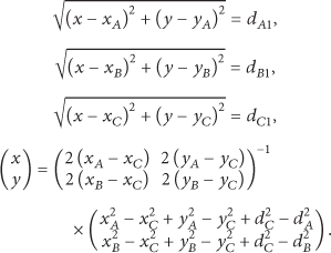

There is a known assumption that

$$\begin{array}{cc}& d_{A\mathrm{1}}=d_{A\mathrm{2}},\\ d_{B\mathrm{1}}=d_{B\mathrm{2}},\\ d_{C\mathrm{1}}=d_{C\mathrm{2}}.\end{array}$$

(39)

So, there is the same coordinates of P1 and P2; clearly, there is a contradiction relationship with known assumptions, so the original theorem is established. That has just finished.

Figure 12

A set of RSSI vector is uniquely correspondent to the coordinates of node.

According to Theorem 4, there is uniqueness for every vector of reference sample points in subsequent localization algorithm.

3.2.2. The Main Idea of the Localization Algorithm

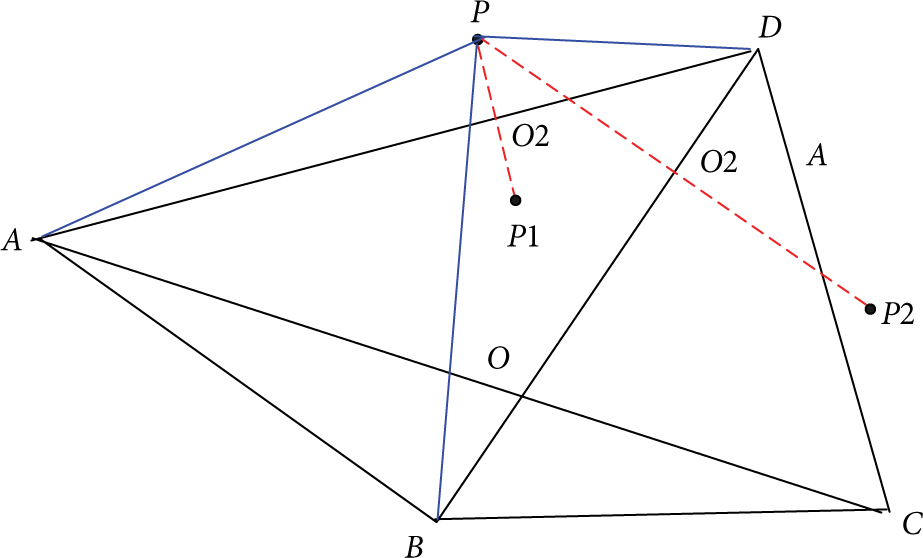
As shown in Figure 13, P1 and P2 are indicated unknown nodes, A, B, C, and D are indicated reference anchor nodes which are the closest to P1 and P2, and the quadrilateral indicated the location unit, which is surrounded by A, B, C, and D. AC and BD indicated two diagonals of the quadrilateral ABCD and O indicated diagonals intersection (coordinates can be obtained); it is regarded as the new reference sample point.

Figure 13

Unknown nodes of P1 and P2 for locating.

By the following relation of area constraint, the location of unknown node can be determined roughly as

$$\begin{array}{cc}& S_{ABCD}=S_{\Delta ABP}+S_{\Delta BCP}+S_{\Delta CDP}+S_{\Delta DAP}.\end{array}$$

(40)

⇒Point P is inside of quadrilateral of ABCD

$$\begin{array}{cc}& S_{\Delta DAO}=S_{\Delta DPA}+S_{\Delta APO}+S_{\Delta OPD}.\end{array}$$

(41)

⇒Point P is inside of $\Delta DAO$ .

By Algorithm 1 of two location system, the location of unknown node can be determined.

Algorithm 1: Decide node in internal or external.

The input: These reference anchor nodes A, B, C, D, which are the closest to $P_i$ , they are made

of a set $C_i$ : $C_i=\{C_{iA},C_{i\mathrm{B}},C_{i\mathrm{C}},C_{i\mathrm{D}}\}$ .

There are number Un unknown nodes are distributed in the region of locating.

The output: The unknown node P is inside of the location unit or external.

Step   1. FOR $i=\mathit{1}$ : Un

Step   2. IF $S_{ABCD}=S_{\mathrm{\Delta }ABP}+S_{\mathrm{\Delta }BCP}+S_{\mathrm{\Delta }CDP}+S_{\mathrm{\Delta }DAP}$

Step   3. RUN InternA

//The algorithm of location mechanism that P is inside of graphics.

Step   4. ELSE

Step   5. RUN ExternA

//The algorithm of location mechanism that P is outside of graphics.

Step   6. ENDIF

Step   7. ENDFOR

3.2.3. The Location Mechanism of the Unknown Node Is inside of the Location Unit

As shown in Figure 14, if the unknown node is inside of ABCD, some operations will be taken to reduce the location unit as follows.

Figure 14

The division of the location unit when the unknown node is inside of graphics and the determination of sample points.

Step 1. Point P is judged whether in $\Delta ABO$ , $\Delta BCO$ , $\Delta CDO$ , and $\Delta DAO$ or not.

Step 2. If point P is inside of any one triangle, three new reference sample points are obtained by taking the middle point of each edge of triangle.

Step 3. The similar degree for the RSSI vector of the unknown node P are compared with the top points of the original triangle and the RSSI vector of three new reference sample points (there are six RSSI vectors); the most similar reference sample points are found; namely, three reference sample points which are closest to P are E, G, D.

By analogy, above steps are repeated, reference sample points are obtained by looking for the midpoint of the location triangle constantly, which are the closest to the unknown node P, the microtriangle region which included the unknown node is narrowed, and Figure 14 has shown that midpoint P is locked in the region of $\Delta LNM$ .

3.2.4. The Location Mechanism of Unknown Node Is outside of the Location Unit

If the unknown node is outside of the unit, as shown in Figure 15, the coordinates of the unknown node is determined by determining two triangles of copoint.

Figure 15

The unknown node is outside of the graph.

Main operations are as follows.

Step 1. Points D and A are found, which are first and second of the RSSI vector of the unknown node P; they are made of $\Delta PAD$ .

Step 2. Points D and B are found, which are first and second of the RSSI vector of the unknown node P; they are made of $\Delta PBD$ .

Step 3. Since the RSSI can be measured, the distance between points can be obtained by the signal attenuation model. Since three lengths of sides are known, the triangle area can be obtained. Since coordinates of two tops are known, the height from point P to its edge can be obtained by the area formulation $S=(\mathrm{1}/\mathrm{2})a\times h$ .

The coordinate of known node is obtained by the following equations:

$$\begin{array}{cc}& L=d_{AD}+d_{DP}+d_{PA},\\ S_{\Delta PAD}=\sqrt{\frac{L}{\mathrm{2}}*\left(\frac{L}{\mathrm{2}}-d_{AD}\right)*\left(\frac{L}{\mathrm{2}}-d_{DP}\right)*\left(\frac{L}{\mathrm{2}}-d_{PA}\right)},\\ S_{\Delta PAD}=\frac{\mathrm{1}}{\mathrm{2}}{d}_{AD}*d_{PO\mathrm{1}},\\ d_{PO\mathrm{1}}=\frac{A*x+B*y+C}{\sqrt{A^{\mathrm{2}}+B^{\mathrm{2}}}}.\end{array}$$

(42)

In this formula, L indicated the circumference of the triangle, S indicated the area of the triangle, d indicated length of sides of the triangle, $A*x+B*y+C=\mathrm{0}$ indicated the linear equation which is included the line $AD$ , and two groups of coordinates of unknown nodes can be obtained by (47).

By the same token, RSSI values of points D and B are chosen, which are first and third in RSSI vector. $\Delta PBD$ is made of points P, D, and B; two groups of coordinates of unknown nodes can be obtained; they are $P(X,Y)$ and $P\mathrm{1}(X\mathrm{2},Y\mathrm{2})$ . The public top point P of two triangles can be obtained by synthesizing two groups of solutions; the coordinate of the unknown node is $P(X,Y)$ .

Although this method is feasible, the rate of measurement error of RSSI on all directions may not be consistent in the process of distance measuring; it will be leaded to distance changes of the corresponding direction showing different conditions; at this time, the above method cannot get two public point of two triangles; namely, there is not public solution for simultaneous equations.

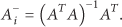
3.2.5. The Method of Generalized Inverse

As shown in Figure 16, there are random measurement errors of RSSI; the calculation result is not coincidence. Furthermore, there is not public solution for simultaneous equations. To this end, a complementary localization algorithm is designed when the node is outside of the location unit by using the generalized inverse [36].

Figure 16

The complementary localization algorithm used the generalized inverse.

$A\in C^{m\times n}$ and $b\in C^m$ are both known; the vector $X\in C^m$ is unknown, which is included in the linear equations $AX=b$ .

If there is a solution of equations, the equation is regarded as the compatibility equations; on the contrary, it is the incompatible equation. In terms of the incompatible equations, there is no general solution. So in this section, the optimal and approximate solution of incompatible and insoluble equations is obtained by using the generalized inverse

$$\begin{array}{cc}& X=\underset{X\in C^m}{\min }\parallel AX-b\parallel .\end{array}$$

(43)

The solution of the above formula is regarded as the least squares solution of incompatible equations; the symbol $\parallel \hspace{0.17em}\parallel$ is the European norm.

Definition 5.

If the incompatible linear equation $AX=b$ is satisfied with $X=A_i^{-}b$ , $A_i^{-}$ indicated the least square generalized inverse of A; there will be a relation that $\tilde{X}$ is satisfied with ${\parallel A\tilde{X}-b\parallel }_{\mathrm{2}}<{\parallel AX-b\parallel }_{\mathrm{2}}$ , so $\tilde{X}=A_i^{-}b$ indicated the least square solution of equations, and there is the minimum sum of squares of error by comparing to other solutions.

G indicated a matrix, $G=A_i^{-}$ , $\tilde{X}=Gb$ indicated the least squares solution of incompatible equations, and ${\parallel AGb-b\parallel }_{\mathrm{2}}$  is minimum, so ${\parallel A(Gb+(I-GA)Z)-b\parallel }_{\mathrm{2}}={\parallel AGb-b\parallel }_{\mathrm{2}}$

Namely, $\tilde{X}=A_i^{-}b$ and $\tilde{X}=(Gb+(I-GA)Z)$ both are least squares solutions of incompatible linear equations.

The coordinate of the unknown node is calculated according to anchor nodes of A, B, and D, and there are equations as follows:

$$\begin{array}{l}\left|k_{AD}*x-y\right|+b_{\mathrm{1}}-h_{AD\perp }*\sqrt{k_{AD}^{\mathrm{2}}+\mathrm{1}}=\mathrm{0},\\ \left|k_{BD}*x-y\right|+b_{\mathrm{2}}-h_{BD\perp }*\sqrt{k_{BD}^{\mathrm{2}}+\mathrm{1}}=\mathrm{0},\\ \mathrm{2}\left(x_A-x_D\right)x+\mathrm{2}\left(y_A-y_D\right)y\\ \hspace{1em}=d_{PA}^{\mathrm{2}}-d_{PD}^{\mathrm{2}}+x_{PD}^{\mathrm{2}}-x_{PA}^{\mathrm{2}}+y_{PD}^{\mathrm{2}}-y_{PA}^{\mathrm{2}},\\ \mathrm{2}(x_B-x_D)x+\mathrm{2}(y_B-y_D)y\\ \hspace{1em}=d_{PB}^{\mathrm{2}}-d_{PD}^{\mathrm{2}}+x_{PD}^{\mathrm{2}}-x_{PB}^{\mathrm{2}}+y_{PD}^{\mathrm{2}}-y_{PB}^{\mathrm{2}}.\end{array}$$

(44)

Above equation set is turned into a form such as the linear equations $AX=b$ ; the coefficient matrix A and vector b are as follows:

$$\begin{array}{cc}& A=\left[\begin{array}{cc}{k}_{AD}& -\mathrm{1}\\ k_{BD}& -\mathrm{1}\\ \mathrm{2}\left(x_A-x_D\right)& \mathrm{2}\left(y_A-y_D\right)\\ \mathrm{2}\left(x_B-x_D\right)& \mathrm{2}\left(y_B-y_D\right)\end{array}\right],\\ b=\left[\begin{array}{c}{h}_{AD\perp }*\sqrt{k_{AD}^{\mathrm{2}}+\mathrm{1}}-b_{\mathrm{1}}\\ h_{BD\perp }*\sqrt{k_{BD}^{\mathrm{2}}+\mathrm{1}}-b_{\mathrm{2}}\\ d_{PA}^{\mathrm{2}}-d_{PD}^{\mathrm{2}}+x_{PD}^{\mathrm{2}}-x_{PA}^{\mathrm{2}}+y_{PD}^{\mathrm{2}}-y_{PA}^{\mathrm{2}}\\ d_{PB}^{\mathrm{2}}-d_{PD}^{\mathrm{2}}+x_{PD}^{\mathrm{2}}-x_{PB}^{\mathrm{2}}+y_{PD}^{\mathrm{2}}-y_{PB}^{\mathrm{2}}\end{array}\right].\end{array}$$

(45)

Because there is no common solution of equations, it is the incompatible linear equations. Then, the least square generalized inverse of equations is as follows:

$$\begin{array}{cc}& A_i^{-}={\left(A^{T}A\right)}^{-\mathrm{1}}{A}^T.\end{array}$$

(46)

So, the least squares solution of incompatible linear equations is as follows:

$$\begin{array}{l}\tilde{X}=A_i^{-}b\\ =A_i^{-}\left[\begin{array}{l}{h}_{AD\perp }*\sqrt{k_{AD}^{\mathrm{2}}+\mathrm{1}}-b_{\mathrm{1}}\\ h_{BD\perp }*\sqrt{k_{BD}^{\mathrm{2}}+\mathrm{1}}-b_{\mathrm{2}}\\ d_{PA}^{\mathrm{2}}-d_{PD}^{\mathrm{2}}+x_{PD}^{\mathrm{2}}-x_{PA}^{\mathrm{2}}+y_{PD}^{\mathrm{2}}-y_{PA}^{\mathrm{2}}\\ d_{PB}^{\mathrm{2}}-d_{PD}^{\mathrm{2}}+x_{PD}^{\mathrm{2}}-x_{PB}^{\mathrm{2}}+y_{PD}^{\mathrm{2}}-y_{PB}^{\mathrm{2}}\end{array}\right].\end{array}$$

(47)

Consider $\tilde{X}=\left[\begin{array}{c}\tilde{x}\\ \tilde{y}\end{array}\right]$ ; the estimation coordinate of the unknown node is $P(\tilde{x},\tilde{y})$ .

4. Results of Simulation Experiment and Real Experiment

4.1. The Result of Simulation Experiment

In order to simulate the real environment, the Shadowing model is used to convert RSSI value into its corresponding distance; ranging errors are setup to simulate the range environment. In this section, localization algorithm is simulated by the tool of MATLAB 7.0, 8 anchor nodes and 160 unknown nodes are taken in this experiment, all nodes are isomorphic, unknown nodes are random distributed in the rectangle area 10 × 10 m² in the experiment environment, and anchor nodes are in the scope of the region that unknown nodes can be communicated (Figure 17).

Figure 17

The layout of anchor nodes and unknown nodes.

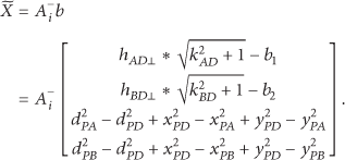
Figure 18 has shown that location error is obtained by simulation when anchor nodes numbers are 8, 16, 24, and 32. Along with the increasing numbers of anchor nodes, location errors are decreased gradually. Because the more the numbers of anchor nodes are in the locating area, the more the numbers of anchor nodes are nearest to the unknown node, the smaller quadrilateral area is formed by anchor nodes; namely, sample reference points are more closer to the unknown node.

Figure 18

The relation between the number of anchor nodes and location error.

In order to describe the effection of ranging error and the trend of ranging error, we have drawn a picture of the relationship between location error and ranging error. In Figure 19, the increasing trends of anchor nodes are increased from 8 to 32, and the changing of the location error is changed.

Figure 19

The relation between RSSI ranging error and location error.

At the same time, under the condition that the total number of unknown nodes is invariable at UN = 160, Figure 19 has shown the simulation result when RSSI ranging errors are 0.1 and 0.2, which are obtained by the method of average calculation, and it also means that the percentages of RSSI ranging error are 10% and 20%. According to Figure 19, when the number of anchor nodes is unchanged, the bigger the RSSI ranging error, the larger the location error; at the same time, when the RSSI ranging error is constant, the more the number of anchor nodes, the smaller the location error. It is also suggested that location error based on RSSI is not only dependent on the localization algorithm, but also dependent on the accuracy of ranging analysis of RSSI [10].

There is a relation analysis between the number of anchor nodes and location error and RSSI range error in Figure 19, in the real measurement environment. The measurement errors of RSSI at all directions are not consistent; the generalized inverse is used to solve the problem that there is not public solution of equations which is formed by the external location unit. The picture of location error is shown from Figures 20, 21, 22, and 23; the colorful lines indicated the mean location error when RSSI ranging errors are 0.05, 0.1, and 0.2, according to these figures, the mean location error = 0.2 is regarded as the better mean value, along with the increasing number of anchor nodes; location error has shown a decreasing trend on the whole; in addition, the final location error of the random ranging error is almost constant with the final location error of the constant ranging error before, but it is practical in application.

Figure 20

The number of anchor nodes is 8.

Figure 21

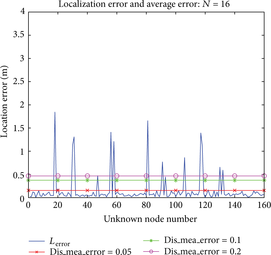
The number of anchor nodes is 16.

Figure 22

The number of anchor nodes is 24.

Figure 23

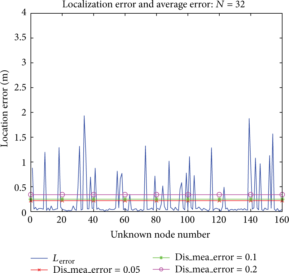
The number of anchor nodes is 32.

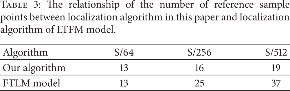
In Table 3, there is a comparative relationship of the number of reference sample points required when each unknown node is required to locate between localization algorithm and localization algorithm of FTLM model. According to Table 3, it can be seen that this algorithm needed less reference sample points when the microarea of positing is the same one; moreover, less amount of calculation is needed. The iteration location by reducing the area is convergent.

Table 3

The relationship of the number of reference sample points between localization algorithm in this paper and localization algorithm of LTFM model.

Algorithm	S/64	S/256	S/512
Our algorithm	13	16	19
FTLM model	13	25	37

When the location area is 10 × 10 m², the comparison of location error between the new algorithm and the sequence three-orthocenter method and the sequence location method and three other center methods is shown, respectively, in Figure 24.

Figure 24

The comparison between algorithms.

Visibly, along with the decreasing number of anchor nodes, location error of these methods will be increased, because the more the number of anchor nodes, the more the times that original location area is divided into different formulas of smaller area, unknown node is more closer to anchor nodes, the more accurate location; Figure 24 has shown that location error of three-orthocenter method is more than five times than new location algorithm when the anchor node number is 8, because the new location algorithm continuously narrowed the area which included the unknown node by the scale of 1/4 in the process of location; thus the actual location of the original node can be better restored; in this paper, the location error of the new location algorithm is almost constant with the sequence three-orthocenter method and the sequence location method when the anchor node number is 32, because the numbers of location sequence of sequence three-orthocenter method and sequence location method are already increased to 462273 when the anchor node number is increased to 32; the area is quite small, which included the unknown node, but, obviously, lots of measurements should be taken; a great amount of calculation and sequence alignment should be made; at this point, the 16 reference sample points are needed to compare with each unknown node in the new location algorithm; the location error is lower than three-orthocenter method; the superiority is shown.

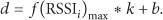
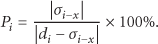
In this simulation experiment, four anchor nodes and four unknown nodes are set up in the region 3 × 3 m². The mean absolute ranging error of nodes is obtained as 0.27 m; the percentage of location error is about 17.6% by the calculation formula:

$$\begin{array}{cc}& P_i=\frac{\left|{\sigma }_{i-x}\right|}{\left|d_i-{\sigma }_{i-x}\right|}\times \mathrm{100}\%.\end{array}$$

(48)

In this formula, $P_i$ indicated the percent of location error of the ith unknown node, ${\sigma }_{i-x}$ indicated the absolute ranging error between real coordinate of the ith unknown node and estimated coordinate, $d_i$ indicated the distance between the ith unknown node and original point.

In Figure 25, black points indicated anchor nodes which are settled before, red points indicated the real coordinates of unknown nodes (they are ranged by tools), and blue triangle indicated estimated coordinates of unknown nodes by the new location algorithm.

Figure 25

The result of location.

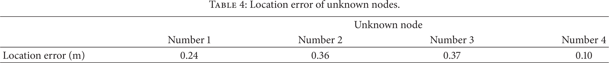
The location error is not only related to the location algorithm but also related to RSSI range and the number of anchors nodes. There is an emulational result of location error of these unknown nodes shown as in Table 4.

Table 4

Location error of unknown nodes.

	Unknown node
	Number 1	Number 2	Number 3	Number 4
Location error (m)	0.24	0.36	0.37	0.10

4.2. The Result of Real Experiment

In this experiment, the latticed experiment environment is designed; there are some nodes in it. Because the place of this experiment is in laboratory, the location grid 20 × 20 m² is set; 4 × 4 m² is just a part of the location grid. In order to choose anchor nodes with better performance, the amount of calculation is needed to decrease; four anchor nodes and one known node are placed in the location grid 4 × 4 m².

In addition, the unknown node is moved at different places. First of all, RSSI values of four nodes in multiple directions are measured, respectively; there is a result that RSSI values of nodes in each direction are basic stability when they are individual, so nodes are required to be immobilized. Secondly, the range models of nodes in different directions are determined, we found that location errors are unreal by calculating, so we measured the RSSI value of four nodes in the range of 1 m and 4 m, respectively, and the total RSSI value of are more than 2000 groups. Thirdly, the statistic of the probability of each RSSI value is obtained by using the tool of Matlab; we selected the optimal value by using the Gaussian fitting. Finally we built the ranging model by introducing $d=\text{RSS}{\text{I}}_i*k+b$ .

In terms of the station that the increasing anchor nodes in the experiment, the range model of this node should be created. Firstly, because interference factors are inevitable indoor, there are different RSSI value of anchor nodes in a different direction. Secondly, the new ranging model of node is needed to build. There are 20 groups of RSSI value of four nodes in the range of 1 m and 4 m, respectively, in Table 5.

Table 5

20 groups of value of signal strength.

Node 1		Node 2		Node 3		Node 4
1 m	4 m	1 m	4 m	1 m	4 m	1 m	4 m
98	33	106	50	106	70	123	70
98	33	106	50	103	70	123	70
100	25	106	50	106	70	123	70
100	25	106	47	106	70	123	70
98	25	106	50	103	56	123	61
98	25	106	53	103	56	123	61
95	22	106	44	103	64	123	61
95	25	106	44	103	64	123	61
98	19	106	44	103	64	123	61
98	19	106	44	103	64	123	61
98	19	106	44	103	64	123	67
98	19	106	44	103	64	123	67
98	19	106	44	103	61	123	67
98	19	106	44	103	61	123	64
98	19	106	44	106	61	123	64
98	19	106	47	106	61	123	64
98	19	106	47	106	58	123	64
98	19	106	47	106	58	123	64
95	19	106	47	106	58	123	64
95	19	106	50	106	58	123	64

The number of nodes and distance of nodes and the probability of each RSSI value are measured in the experiment. For example, there are parts of information from Tables 6, 7, 8, and 9.

Table 6

The measured data of number 1 node.

Number	Distance	Value	Count	Percent
1	1 m	67	4	1.00%
		72	80	20.00%
		75	8	2.00%
		78	10	2.50%
		81	20	5.00%
	4 m	50	4	1.00%
		58	21	5.25%
		64	37	9.25%
		67	70	17.50%
		70	121	30.25%
		72	147	36.75%

Table 7

The measured data of number 2 node.

Number	Distance	Value	Count	Percent
2	1 m	100	15	3.75%
		103	81	20.25%
		106	300	75.00%
		109	4	1.00%
		36	9	2.25%
	4 m	39	48	12.00%
		42	20	5.00%
		44	52	13.00%
		47	25	6.25%
		50	129	32.25%
		53	82	20.50%

Table 8

The measured data of number 3 node.

Number	Distance	Value	Count	Percent
3	1 m	14	16	4%
		70	36	9.00%
		72	21	5.25%
		75	15	3.75%
		78	81	20.25%
	4 m	81	67	16.75%
		86	91	22.75%
		89	32	8.00%
		92	19	4.75%
		95	22	5.50%
		81	86	21.50%

Table 9

The measured data of number 4 node.

Number	Distance	Value	Count	Percent
4	1 m	100	4	1.00%
		103	182	40.50%
		106	50	12.50%
		123	164	41.00%
		61	75	18.75%
	4 m	64	79	19.75%
		67	127	31.75%
		70	59	14.75%
		72	60	15.00%
		100	4	1.00%
		103	182	40.50%

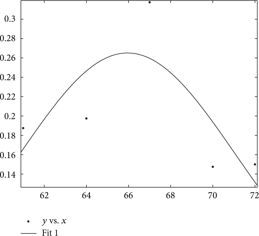
The optimal value is selected by using the Gaussian fitting. Figures 26, 27, 28, 29, 30, 31, 32, and 33 have shown curves of Gaussian fitting of four nodes when their distances are 1 m and 4 m.

Figure 26

The fitting curve of number 1 node when distance is 1 m.

Figure 27

The fitting curve of number 1 node when distance is 4 m.

Figure 28

The fitting curve of number 2 node when distance is 1 m.

Figure 29

The fitting curve of number 2 node when distance is 4 m.

Figure 30

The fitting curve of number 3 node when distance is 1 m.

Figure 31

The fitting curve of number 3 node when distance is 4 m.

Figure 32

The fitting curve of number 4 node when distance is 1 m.

Figure 33

The fitting curve of number 4 node when distance is 4 m.

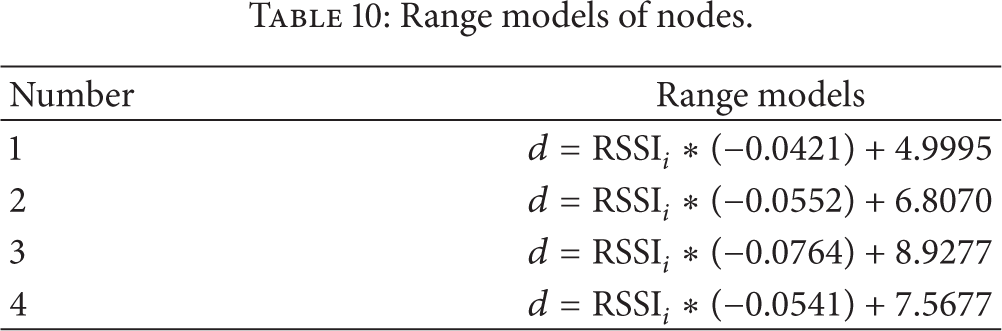
The piecewise linear interpolation for RSSI-d curve is used to ensure the ranging precision. There are four range models of four nodes as in Table 10.

Table 10

Range models of nodes.

Number	Range models
1	$d={\text{RSSI}}_i\mathrm{*}(-\mathrm{0.0421})+\mathrm{4.9995}$
2	$d={\text{RSSI}}_i\mathrm{*}(-\mathrm{0.0552})+\mathrm{6.8070}$
3	$d={\text{RSSI}}_i\mathrm{*}(-\mathrm{0.0764})+\mathrm{8.9277}$
4	$d={\text{RSSI}}_i\mathrm{*}(-\mathrm{0.0541})+\mathrm{7.5677}$

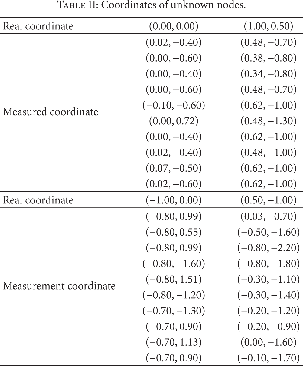
There are real coordinates of nodes. There is part of measurement data in Table 11.

Table 11

Coordinates of unknown nodes.

Real coordinate	$(\mathit{0.00,0.00})$	$(\mathit{1.00,0.50})$
Measured coordinate	$(\mathit{0.02},-\mathit{0.40})$	$(\mathit{0.48},-\mathit{0.70})$
	$(\mathit{0.00},-\mathit{0.60})$	$(\mathit{0.38},-\mathit{0.80})$
	$(\mathit{0.00},-\mathit{0.40})$	$(\mathit{0.34},-\mathit{0.80})$
	$(\mathit{0.00},-\mathit{0.60})$	$(\mathit{0.48},-\mathit{0.70})$
	$(-\mathit{0.10},-\mathit{0.60})$	$(\mathit{0.62},-\mathit{1.00})$
	$(\mathit{0.00,0.72})$	$(\mathit{0.48},-\mathit{1.30})$
	$(\mathit{0.00},-\mathit{0.40})$	$(\mathit{0.62},-\mathit{1.00})$
	$(\mathit{0.02},-\mathit{0.40})$	$(\mathit{0.48},-\mathit{1.00})$
	$(\mathit{0.07},-\mathit{0.50})$	$(\mathit{0.62},-\mathit{1.00})$
	$(\mathit{0.02},-\mathit{0.60})$	$(\mathit{0.62},-\mathit{1.00})$
Real coordinate	$(-\mathit{1.00,0.00})$	$(\mathit{0.50},-\mathit{1.00})$
Measurement coordinate	$(-\mathit{0.80,0.99})$	$(\mathit{0.03},-\mathit{0.70})$
	$(-\mathit{0.80,0.55})$	$(-\mathit{0.50},-\mathit{1.60})$
	$(-\mathit{0.80,0.99})$	$(-\mathit{0.80},-\mathit{2.20})$
	$(-\mathit{0.80},-\mathit{1.60})$	$(-\mathit{0.80},-\mathit{1.80})$
	$(-\mathit{0.80,1.51})$	$(-\mathit{0.30},-\mathit{1.10})$
	$(-\mathit{0.80},-\mathit{1.20})$	$(-\mathit{0.30},-\mathit{1.40})$
	$(-\mathit{0.70},-\mathit{1.30})$	$(-\mathit{0.20},-\mathit{1.20})$
	$(-\mathit{0.70,0.90})$	$(-\mathit{0.20},-\mathit{0.90})$
	$(-\mathit{0.70,1.13})$	$(\mathit{0.00},-\mathit{1.60})$
	$(-\mathit{0.70,0.90})$	$(-\mathit{0.10},-\mathit{1.70})$

Through times of measurement of the unknown node, the smallest location error is regarded as the ideal date which is obtained from the noninterfering environment. For the first time, the smallest location error is 0.4 m in the actual coordinates of node; for the second time, the smallest location error is 1.31 m; for the third time, the smallest location error is 0.59 m; for the fourth time, the smallest location error is 0.48 m (see Table 12).

Table 12

Coordinates of four nodes.

	Number
	NO. 1	NO. 2
Real coordinate	$(\mathit{0.00,0.00})$	$(\mathit{1.00,0.50})$
Mean coordinate	$(\mathit{0.07},-\mathit{0.50})$	$(\mathit{0.62},-\mathit{1.00})$
Maximum (m)	0.72	1.87
Minimum (m)	0.40	1.31
Mean (m)	0.52	1.53
	Number
	NO. 3	NO. 4
Real coordinate	$(-\mathit{1.00,0.00})$	$(\mathit{0.05},-\mathit{1.00})$
Mean coordinate	$(-\mathit{0.80,0.99})$	$(-\mathit{0.10},-\mathit{1.70})$
Maximum (m)	1.61	1.84
Minimum (m)	0.59	0.48
Mean (m)	1.04	1.02

In Table 9, since interference factors are inevitable indoor, there are different RSSI values of anchor nodes in different direction. Their ranging models are based on different nodes. There are different results of mean location error.

In Figure 34, black squares indicated fixed anchor nodes in the experiments, yellow dots indicated actual coordinates of unknown nodes, and blue triangle points indicated estimation coordinates of unknown nodes which are obtained by the new location algorithm. In each experiment, the mean location error is about 1 m. Four yellow dots indicated movement results; there are four times of movement for the unknown node; the experiment is regarded as a dynamic test.

Figure 34

The effect of location.

4.3. The Simulated Application of the Location Algorithm

4.3.1. The Design of Location System

The location system is applied at home and location area is set as 4 × 4 m². Four anchor nodes are It is selected in the location region. A RFID tag is carried with robot which is regarded as the unknown node. In addition, the location system is set as a server and a transmission PC and a router (see Figure 35). Firstly, anchor nodes send strength signal to the robot which can be received and sent signal. Secondly, the server received signal information from the robot and processed these data. Thirdly, mobile terminal gets processed data from server by router. Finally, information of mobile robot is displayed in the interface of mobile terminal. Particularly, the card reader is set at the door; it is a caution of the mobile robot when the robot is outside of the location region.

Figure 35

The schematic diagram of the location system.

4.3.2. The Design of Mobile Terminal

This system can be applied to prevent children lost indoor; accounting that the children's speed of movement is relatively much slower than parents, the process of implement is regarded as a lower level dynamic environment. The system is able to work well when child moves into room.

There are some pictures of experiment displayed in the interface of mobile terminal. In Figure 36, the application is set at home, so the background of the interface is the picture of home, and the black point indicated the mobile robot.

Figure 36

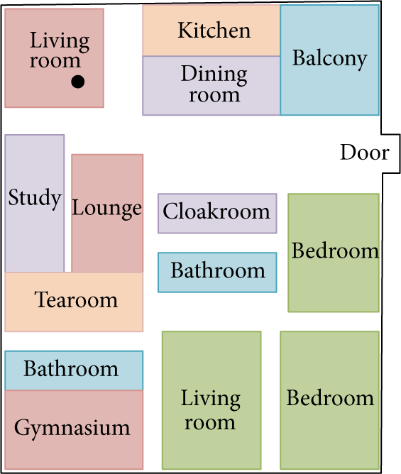
The normal effect.

In Figure 37, it is shown that there is an alarm's tooltip in the picture; it indicated that the RFID tag is read by card reader; namely, the mobile robot is outside of home. Particularly, this system designed the alarm's music with the alarm's function.

Figure 37

The alarm's effect.

5. Conclusion

In this paper, we studied on the location technology of RSSI-based in WSN. In order to get accurate RSSI value and simulate the real experimental environment, there is a large amount of experimental data. In the process of location, we determined the related parameters of the Shadowing model and analyzed the RSSI value at the specific distance by the Gaussian fitting; in addition, not only we built the RSSI-based interpolation model of node, but also we analyzed the influence of the number of nodes. In terms of the new location algorithm, we proposed the location mechanism; it is used to estimate that the unknown node is internal or external. Moreover, we proposed the concept of vector similar degree; it is helpful to choose anchor nodes. Particularly, the generalized inverse is solved to estimate the coordinate of unknown node by equations. Simulation and experiment results show that our approach outperforms existing approaches in terms of location accuracy, and our location system is applied to locate the robot quite well.