Sage Journals: Discover world-class research

Abstract

Multibranch interconnected hydropneumatic suspension (MIHS) is increasingly applied in heavy multiaxle vehicle (HMV) for its superior characteristics, such as adjustable damping, and the antiroll and balancing axle load ability. However, as for multibranch hydropneumatic suspension, the stiffness and damping are coupled with each other tightly, which represents damping noncoincidence (DNC) problem. The DNC problem has become a key obstacle for developing suspension control technology and improving suspension performance. Firstly, a kind of MIHS structure is developed for an HMV, and the interconnected structure and principle are explained. Then the DNC problem is proposed and is given a description. And then, according to the researching needs, the suspension system model of single cylinder connected with multiple branches is built up based on the knowledge of state change of fluid and gas. Fourthly, the root cause of DNC problem is given according to simulation results. Fifthly, the impacts of three factors on DNC problem are studied, respectively, by adjusting excitation signal and system parameters in the simulation. The simulation results are quantitatively compared with regard to damping noncoincidence rate (DNCR). In the end, some conclusions are drawn based on the discussion and analysis and the future work is proposed.

1. Introduction

With the increase in the need of comfort and handling performance, significant challenges are proposed in the vehicle suspension design. The performance characteristics of an HMV are strongly related to its roll and pitch motion.

The advent of hydropneumatic suspension (HS) has had a significant impact on the technological advance of HMV. A great number of studies on the HS have been developed to realize compact suspension with integrated pneumatic spring and hydraulic damping to achieve improved comfort and handling performance [1 –3]. Amounts of study have proved that such construction has large size cylinders which require excessive working pressure [4, 5]. The scheme of passive load-sharing spring in parallel to HS has also been suggested in order to reduce operating pressure. The results have revealed that the additional spring significantly limits the effectiveness of the roll connection [5, 6]. Besides, a kind of pitch-interconnected HS with adjustable damping valve has been developed to improve the comfort performance and to resolve the problem of axle load distribution [7 –9]. Such HS is coupled with antiroll bars to improve vehicle roll stability and to balance the roll moment distribution between front and rear axles [10]. However, the use of antiroll bars adds considerable weight and deteriorates ride comfort to the vehicle to some extent. Moreover, the use of strong stiff antiroll bar would significantly reduce the effectiveness of roll damping, which is undesirable for the control of dynamic roll response of HMV [11, 12].

The development of IHS has been explored during the past decade. The IHS is a kind of suspension where the roll connection is coupled with pitch connection. The IHS achieves antiroll and antipitch performance, and the antiroll bars exist no longer. Such construction supplies more space for chassis arrangement. There are a few of available literatures contributing to research of IHS. Cao investigated the theoretical analysis and dynamics simulation of IHS [13 –18]. Zhang et al. did some research on modeling and bench test as to IHS. The presented approach provides a scientific basis for investigating the dynamic characteristics of vehicles equipped with IHS, and the results offer further confirmation that interconnected suspension schemes can provide, at least to some extent, individual control of model stiffness and damping characteristics [19 –23].

However, as for IHS, the parameters setting of multibranch structure and characteristics of stiffness-damping coupling lead to DNC problem. The damping force curve responding to piston velocity from zero to maximum does not coincide with the damping force curve responding to piston velocity from maximum to zero. The DNC brought new problem to suspension control technology. It increased the difficulty to ensure control accuracy for the damping forces difference of the two parts of a whole compression stroke.

Based on the analysis above, it can be drawn that the DNC is a problem which is worth doing some research.

This paper proposes an IHS for HMV and a description of the basic construction and the principle of the HIS are supplied consequently. The problem of DNC is proposed and given a strict definition. For the need of research, the model is developed. Based on the model, the root cause of DNC is figured out and main influence factors are studied, respectively. Finally, the conclusions with the discussion above and future research work are drawn.

2. Description of IHS System

With the considerably practical benefits of the IHS in antiroll and antipitch performance of HMV, in this section, the construction design and working principle of hydraulic system of IHS are presented, including interconnected type of hydraulic systems and various valves.

For the need of some special functions, a kind of IHS system is designed for a heavy four-axle vehicle. The vehicle and hydraulic integration blocks are shown in Figure 1.

Figure 1:

Vehicle and hydraulic integration blocks.

Figure 2 illustrates the schematic of the hydraulic system used in the front two axles of a heavy four-axle vehicle. It consists of four cylinders (1R, 2R, 1L, and 2L), three hydraulic integration blocks (FR, FM, and FL), and pipes connecting cylinders to blocks.

Figure 2:

Schematic of hydraulic system design.

All the valves and their functions in the system are listed in Table 1.

Table 1:

Valves and function in the system.

Name	Symbol	Number	Function

2/2 electromagnetic valve	V1r, V2r, V1l, V2l, S-V1r, S-V2r, S-V1l, S-V2l, Vfr-s, Vfl-s, Vld, Vlu, Vrd, Vru	14	Cut or connect the oil lines

2/3 electromagnetic valve	C-V1r, C-V2r, C-V1l, C-V2l	4	Change the connected form

Check-throttle valve	T-V1r, T-V2r, T-V1l, T-V2l, T-Vfr-b, T-Vfr-t, T-Vfl-b, T-Vfl-t	8	Supply damping

Relief valve	F-V1r, F-V2r, F-V1l, F-V2l, P-Vfr-c, P-Vfr-d, P-Vfl-c, P-Vfl-d	8	Supply damping

The upper chamber of cylinder is piston chamber, while the lower chamber is rod chamber. The connecting forms of system can be expressed differently by controlling the electromagnetic valves. The connected forms are described in Figure 3.

Figure 3:

Schematic of connected form.

In Figure 3(a), the suspension system is expressed as the independent form by controlling electromagnetic valves S-V1r, C-V1r, S-V2r, C-V2r, S-V1l, C-V1l, S-V2l, and C-V2l. As for this type, the upper chamber and lower chamber of every cylinder are connected with an accumulator, while the four cylinders respond to road impact independently. In Figure 3(b), the suspension system is expressed as the balancing form by controlling electromagnetic valves Vld, Vlu, Vrd, and Vru. As for this type, the upper chamber of 1R connects to the upper chamber of 2R on the right side, as well as the left side. This type has an effect on antiroll motion when used in two-axle vehicles and also influences the balancing axle load when used in multiaxle vehicles. In Figure 3(c), the suspension system is expressed as the antiroll form at rear axle and the independent form at front axle by controlling electromagnetic valves S-V1r, C-V1r, S-V1l, and C-V1l. As for this type, the cylinders 1R and 1L are kept as the independent form and the upper (lower) chamber of 2R connects to the lower (upper) chamber of 2L that makes up the antiroll form. This type impacts on the rolling motion of the vehicle. In Figure 3(d), the suspension system is expressed as the interconnected form by controlling all the electromagnetic valves at “on” state. As for this type, the upper chamber of 1R connects to the upper chamber of 2R. The lower chamber of 1R connects to the lower chamber of 2R. The upper chambers of the right side cylinders (1R, 2R) connect to the lower chambers of the left side cylinders (1L, 2L). The lower chambers of the cylinders on the right side connect with the upper chambers of the cylinders on the left side. Since the cylinders on the left side have the same connecting form as the cylinders on the right side, there is no need to explain much more here. In this connecting form, the suspension system can be capable of balancing axle load and also has the antiroll function.

3. Statement of DNC Problem

Firstly, some foundational knowledge and definition will be given here. The motion of piston conforming to simple harmonic vibration is described in Figure 4. The compression stroke is marked with blue line, and the rebound stroke is marked with red line. The travel from − x_{max ⁡} to 0 is defined as lower part of compression stroke, and the travel from 0 to x_{max ⁡} is defined as upper part of the compression stroke. Meanwhile, the same condition happens to the rebound stroke.

Figure 4:

Description of piston motion status.

Over the past decades, many studies have been carried out on the damping characteristics of hydropneumatic suspension. The research mainly focused on independent hydropneumatic suspension. Damping characteristics responding to piston motion status are described in Figure 5. The x-axis is piston velocity, and the y-axis is damping force. The damping force reaches the maximum value when piston moves to static balancing position, and damping force reaches the minimum value when piston moves to upper or lower limit position. For example, to compression stroke, a whole compression stroke contains velocity range which changes from 0 to maximum and back to 0. The two damping curves coincide into one curve as in the first quadrant.

Figure 5:

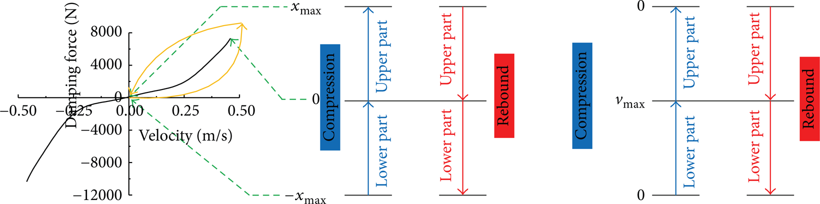
Damping characteristics responding to piston motion status.

However, as for IHS, we found that the damping force curves are not coincident with each other, which is described in Figure 6. Taking the compression stroke as an example, the damping force curve responding to piston velocity from 0 to maximum does not coincide with the damping force curve responding to piston velocity from maximum to 0, which is defined as DNC problem. The rebound stroke has the same condition. So, to discover the root cause for the DNC is one purpose of this paper. And to find out the influence factors corresponding to DNC is another.

Figure 6:

Damping characteristic comparison.

4. Multibranch HS System Model

From Figure 2 we can see that the four cylinders have the same connected condition. One whole compression stroke of cylinder is the focus of the investigation on the DNC problem. Owing to the symmetrical structure and system characteristics, hydraulic line of cylinder 1R piston side is taken as an object of research. The piston chamber connects to three accumulators through three lines. The damping force for compression stroke mainly comes from the valves T-V1r, F-V1r, T-V2r, F-V2r, T-Vfr-b, and P-Vfr-c. The damping force coming from the upper chamber line can be neglected owing to the check valve T-Vfr-t. Besides, all insignificant electromagnetic valves are left out of the system. For that, the physical model used for DNC problem is described as Figure 7. There are one accumulator and three kinds of valves in every branch. When the cylinder moves in the compression stroke, the oil flows from cylinder chamber to three accumulators through three branches. The gas in accumulators is compressed due to oil flow, which produces the elastic force. The damping force results from the oil flowing through the valves in every branch.

Figure 7:

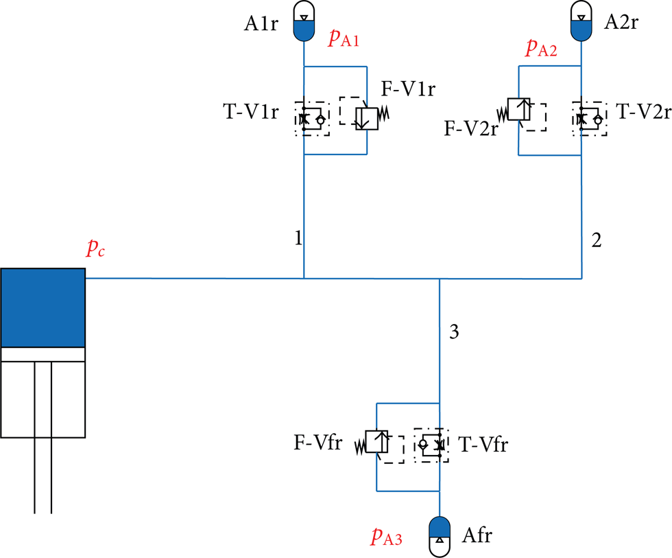
The hydraulic schematic of single cylinder multibranch for compression stroke.

4.1. Model of Accumulator

The accumulator is full of nitrogen which can be treated as ideal gas when both pressure and working temperature have limited variation range. In rapid loading process, it can be treated as isolated and the polytropic index of gas γ = 1.4 is chosen. Meanwhile, the slow loading process can be treated as isothermal and we choose the polytropic index of gas γ = 1.0. The actual process is a condition between isolated and isothermal process and polytropic index of gas is chosen as γ = 1.2 ∼ 1.3 [24, 25].

According to gas state equation, we can obtain

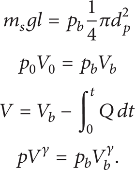
\begin{matrix} m_{s} g l = p_{b} \frac{1}{4} π d_{p}^{2} \\ p_{0} V_{0} = p_{b} V_{b} \\ V = V_{b} - \int_{0}^{t} Q d t \\ p V^{γ} = p_{b} V_{b}^{γ} . \end{matrix}

(1)

From (1) we can get gas pressure equation of accumulator at random time:

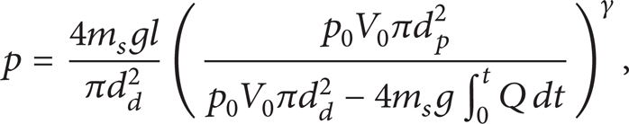
p = \frac{4 m_{s} g l}{π d_{d}^{2}} {(\frac{p_{0} V_{0} π d_{p}^{2}}{p_{0} V_{0} π d_{d}^{2} - 4 m_{s} g \int_{0}^{t} Q d t})}^{γ},

(2)

where m_s is spring mass of single wheel; l is the lever rate; d_p is diameter of piston; p₀ is precharge pressure of accumulator; V₀ is original volume of accumulator; p_b is gas pressure at static balance; V_b is gas volume at static balance; p is gas pressure at random time; V is gas volume at random time; Q is the oil flow which flows into the accumulator; γ is gas polytropic index.

4.2. Model of Throttle Valve

The principle of throttle valve can be equivalent to a hole. According to Bernoulli equation, the flow-pressure relationship can be described as

Q_{t} = C_{d} \frac{1}{4} π d_{t}^{2} \sqrt{\frac{2 Δ p}{ρ}},

(3)

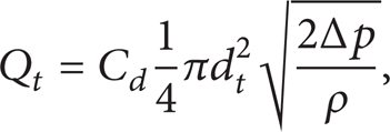
where Q_t is the flow that flows through the hole; C_d is the flow coefficient; d_t is the diameter of the hole; Δp is pressure difference between two sides of the hole; ρ is the oil density.

4.3. Model of Check Valve and Relief Valve

Both models of check valve and relief valve can be built up as a poppet valve with preloaded spring which is expressed in Figure 8. Owing to the symmetrical structure of poppet valve about the middle axis, the fluid velocity and pressure distribute along the radial symmetrically. For that, we just need to study the radial force of spool [26 –28]. The motion states of check valve are separated to three steps: close, open, and full open.

Figure 8:

Diagram of check valve.

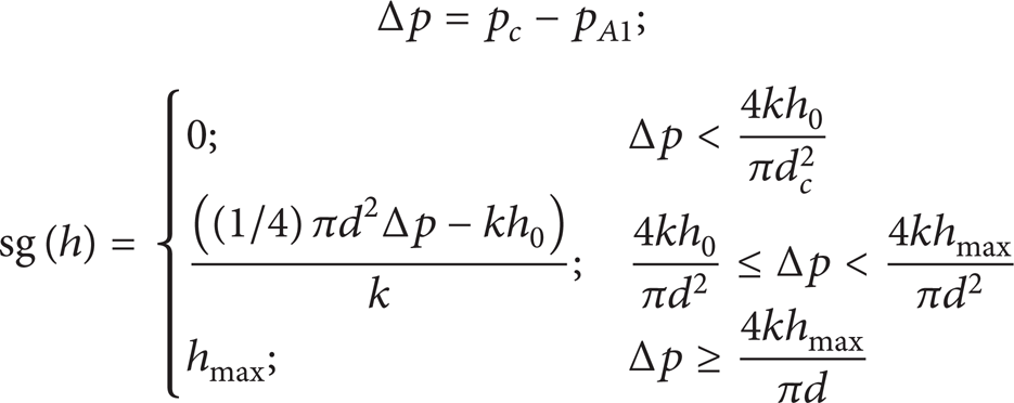
As for poppet valve, flow and pressure difference still has the relationship as

Q_{c} = C_{d} π d_{c} h \sqrt{\frac{2 Δ p}{ρ}} .

(4)

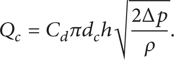
When the pressure difference between inlet and outlet is lower than the limit value, the spool distance is h = 0. When the pressure difference between inlet and outlet is higher than the limit value, the spool distance is h = h_i. When the pressure difference between inlet and outlet continues to increase, the spool distance reaches maximum h = h_max-c. The relationship between the flow and pressure difference of check valve can be obtained as

Q_{r} = \{\begin{cases} 0; & Δ p < \frac{4 k h_{0}}{π d_{r}^{2}} \\ C_{d} π d_{r} h_{i} \sqrt{\frac{2 Δ p}{ρ}}; & \frac{4 k h_{0}}{π d_{r}^{2}} \leq Δ p < \frac{4 k h_{\max}}{π d_{r}^{2}} \\ C_{d} π d_{r} h_{\max} \sqrt{\frac{2 Δ p}{ρ}}; & Δ p \geq \frac{4 k h_{\max}}{π d_{r}^{2}} \end{cases})

(5)

and h_i = ((1/4)πd_r²Δp − kh₀)/k.

Here Q_r is the flow that flows through the valve; d_r is the diameter of the hole; h_{max ⁡} is the maximum distance of the spool; k is the stiffness of the preloaded spring; h₀ is the original length of the precompressed spring; h_i is the spool distance at the open state.

4.4. Model of Suspension System

Based on the valve model and the connected structure above, the model of hydropneumatic suspension with single cylinder connected with multibranch is given as follows.

Because the flow is the function of differential pressure Δp, for simplicity, the flow of every valve is written as function of differential pressure Δp.

The relationship of flow and pressure difference for branch A1r is given in

\begin{matrix} Q_{T 1} = sign (x_{p}) f_{T 1} (|Δ p|) \\ Q_{C 1} = sign (x_{p}) f_{C 1} [|Δ p|, sg (h)] \\ Q_{R 1} = sign (x_{p}) f_{R 1} [|Δ p|, sg (h)] \\ Q_{1} = Q_{T 1} + Q_{C 1} + Q_{R 1} \\ p_{A 1} = \frac{4 m_{s} g l}{π d_{p}^{2}} {(\frac{p_{0 - A 1} V_{0 - A 1} π d_{p}^{2}}{p_{0 - A 1} V_{0 - A 1} π d_{p}^{2} - 4 m_{s} g \int_{0}^{t} Q_{1} d t})}^{γ}, \end{matrix}

(6)

where Q_T1 is the flow which flows through the throttle valve in branch A1r; Q_C1 is the flow which flows through the check valve in branch A1r; Q_R1 is the flow which flows through the relief valve in branch A1r; Q₁ is the total flow which flows through the branch A1r; p_A1r is the pressure in accumulator A1r.

And the symbol definition also applies to (7) and (8). Equation (7) is used to judge from the state of check valve and relief valve. Equation (8) is used to judge from the compression and rebound stroke. Consider

\begin{matrix} Δ p = p_{c} - p_{A 1}; \\ sg (h) = \{\begin{cases} 0; & Δ p < \frac{4 k h_{0}}{π d_{c}^{2}} \\ \frac{((1 / 4) π d^{2} Δ p - k h_{0})}{k}; & \frac{4 k h_{0}}{π d^{2}} \leq Δ p < \frac{4 k h_{\max}}{π d^{2}} \\ h_{\max}; & Δ p \geq \frac{4 k h_{\max}}{π d} \end{cases}) \end{matrix}

(7)

sign (x_{p}) = \{\begin{cases} 1; & x_{p} > 0 \\ 0; & x_{p} = 0 \\ - 1; & x_{p} < 0 . \end{cases})

(8)

Similarly, the relationship of flow and pressure difference for branch A2r is given in

\begin{matrix} Q_{T 2} = sign (x_{p}) f_{T 2} (|Δ p|) \\ Q_{C 2} = sign (x_{p}) f_{C 2} [|Δ p|, sg (h)] \\ Q_{R 2} = sign (x_{p}) f_{R 2} [|Δ p|, sg (h)] \\ Q_{2} = Q_{T 2} + Q_{C 2} + Q_{R 2} \\ p_{A 2} = \frac{4 m_{s} g l}{π d_{p}^{2}} {(\frac{p_{0 - A 2} V_{0 - A 2} π d_{p}^{2}}{p_{0 - A 2} V_{0 - A 2} π d_{p}^{2} - 4 m_{s} g \int_{0}^{t} Q_{2} d t})}^{γ}; \\ Δ p = p_{c} - p_{A 2} . \end{matrix}

(9)

Similarly, the relationship of flow and pressure difference for branch A3r is given in

\begin{matrix} Q_{T 3} = sign (x_{p}) f_{T 3} (|Δ p|) \\ Q_{C 3} = sign (x_{p}) f_{C 3} [|Δ p|, sg (h)] \\ Q_{R 3} = sign (x_{p}) f_{R 3} [|Δ p|, sg (h)] \\ Q_{3} = Q_{T 3} + Q_{C 3} + Q_{R 3} \\ p_{A 3} = \frac{4 m_{s} g l}{π d_{p}^{2}} {(\frac{p_{0 - A 3} V_{0 - A 3} π d_{p}^{2}}{p_{0 - A 3} V_{0 - A 3} π d_{p}^{2} - 4 m_{s} g \int_{0}^{t} Q_{3} d t})}^{γ}; \\ Δ p = p_{c} - p_{A 3} . \end{matrix}

(10)

By checking (6), (9), and (10), we should work out the pressure of cylinder piston chamber to connect the cylinder model and valve model (Figure 9).

Figure 9:

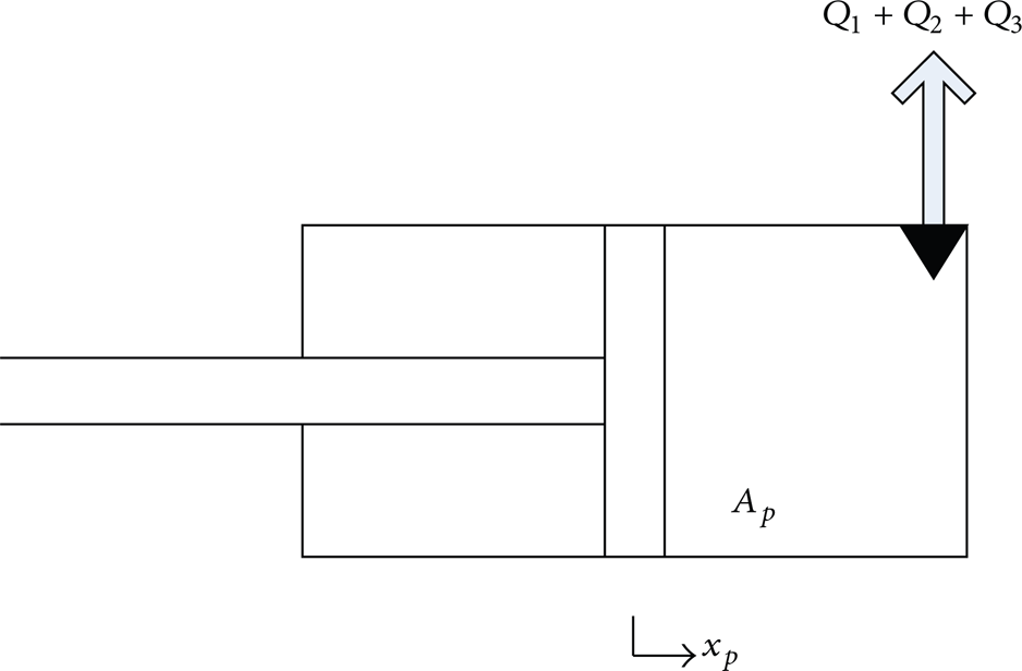
Diagram of cylinder.

The pressure difference equation of cylinder piston chamber is described in

\begin{matrix} {\dot{p}}_{c} = \frac{1}{C_{HC}} [{\dot{x}}_{p} A_{p} - (Q_{1} + Q_{2} + Q_{3})] \\ C_{HC} = \frac{V_{b} - x_{p} A_{p}}{K_{oil}} \\ {(p_{c}|}_{t = 0} = \frac{4 m_{s} g l}{π d_{p}^{2}}, \end{matrix}

(11)

where C_HC is volume modulus; V_b is cylinder volume at static equilibrium, K_oil is bulk modulus of oil.

Based on (6), (9), (10), and (11), by analyzing the relationship of input and output, the flow diagram of model of single cylinder connected with multibranch is shown in Figure 10.

Figure 10:

Flow diagram of model of single cylinder connected with multibranch.

The system model of single cylinder connected with multibranch is implemented in Matlab/Simulink as Figure 11.

Figure 11:

System model implemented in Matlab/Simulink.

5. The Root Cause of DNC Problem

In order to study the DNC problem, the simulation results are compared in two different cases. (1) The parameters of all valves and accumulators in the three branches are set as the same. (2) The damping parameters of Afr branch are set bigger than the other two branches. The parameters used in simulation are listed in Tables 2 and 3.

Table 2:

Parameters for case 1.

Symbol	Value

ρ (kg/m³)	850
C _d	0.62
d_{t − A1r}, d_{t − A2r}, d_{t − Afr} (m)	0.007
d_{c − A1r}, d_{c − A2r}, d_{c − Afr} (m)	0.01
d_{r − A1r}, d_{r − A2r}, d_{r − Afr} (m)	0.006
h_{max ⁡ − c − A1r}, h_{max ⁡ − c − A2r}, h_{max ⁡ − c − Afr} (m)	0.003
h_{max ⁡ − r − A1r}, h_{max ⁡ − r − A2r}, h_{max ⁡ − r − Afr} (m)	0.0025
d_p (m)	0.115
m_s (kg)	2957
p_{0 − A1r}, p_{0 − A2r}, p_{0 − Afr} (bar)	35
V_{0 − A1r}, V_{0 − A1r}, V_{0 − A1r} (L)	1.4
γ	1.3

Table 3:

Parameters for case 2.

Symbol	Value

ρ (kg/m³)	850
C _d	0.62
d_{t − A1r}, d_{t − A2r} ∖ d_{t − Afr} (m)	0.007 ∖ 0.005
d_{c − A1r}, d_{c − A2r}, d_{c − Afr} (m)	0.01
d_{r − A1r}, d_{r − A2r}, d_{r − Afr} (m)	0.006
h_{max ⁡ − c − A1r}, h_{max ⁡ − c − A2r}, h_{max ⁡ − c − Afr} (m)	0.003
h_{max ⁡ − r − A1r}, h_{max ⁡ − r − A2r} ∖ h_{max ⁡ − r − Afr} (m)	0.0025∖0.002
d_p (m)	0.115
m_s (kg)	2957
p_{0 − A1r}, p_{0 − A2r} ∖ p_{0 − Afr} (bar)	35 ∖ 50
V_{0 − A1r}, V_{0 − A1r}, V_{0 − A1r} (L)	1.4
γ	1.3

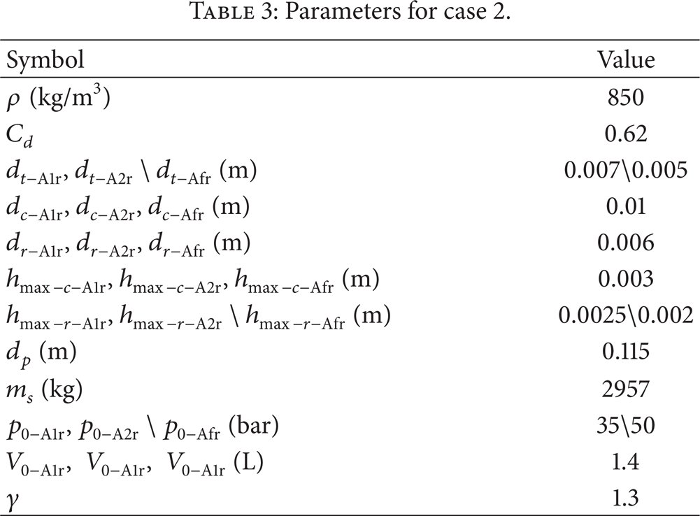
The differences of the two sets of parameters are the diameters of throttle valve, maximum distance of the relief valve spool, and the precharge pressure of accumulator in Afr branch. The resistance of oil flowing in Afr branch is bigger than both of that in A1r and that in A1r branch.

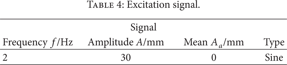
The excitation signal of piston displacement is given in Table 4.

Table 4:

Excitation signal.

Signal
Frequency f/Hz	Amplitude A/mm	Mean A_a/mm	Type

2	30	0	Sine

In Figure 12, the first column (a1)∼(d1) shows the system characteristics in case 1. The second column (a2)∼(d2) shows the system characteristics in case 2, where (a1) and (a2) are piston displacement; (b1) and (b2) are accumulator pressure; (c1) and (c2) are the flow of the three branches; (d1) and (d2) are the damping power of the valve union in the three branches. There are three curves in every figure. The black curve represents the situation of branch A1r, and the red curve represents the situation of branch A2r; besides, the blue curve represents the situation of branch Afr.

Figure 12:

System variables comparison of the two cases.

The abscissa in every figure represents time. Because the frequency of excitation signal is 2 Hz, the time range of one whole compression stroke is 0.375 s∼0.625 s which is marked by red vertical dashed line. Among those, from 0.375 s∼0.5 s is the lower part of the compression stroke and from 0.5 s∼0.625 s is the upper part of the compression stroke. The time point corresponding to static balance is marked with green vertical dashed line.

Let us see the first column in Figure 12 firstly. In (a1), the piston displacement changes from the lower limit position at 0.375 s to the upper limit position at 0.625 s. Correspondingly, the pressure of the three accumulators increases straightly during the time 0.375 s∼0.625 s in (b1). And the three pressure curves are coincident, which means that the pressure of the three accumulators changes synchronously. Then, in (c1), the flow of the three branches increases from 0.375 s to 0.5 s and decreases from 0.5 s to 0.625 s. It is easy to see that the three flow curves are coincident, which means the flows of the three branches are the same and change synchronously. And then, the power curves are shown in (d1). We can see that the three power curves are coincident, and the area of the left part is same as the area of the right part, which means the damping of the lower part is equivalent to the damping of the upper part in one whole compression stroke.

Then, let us see the second column in Figure 12. From (b2) we can see that the pressure curve of accumulator Afr is not coincident with the other two pressure curves of accumulator A1r and accumulator A2r. When the compression stroke finishes at 0.625 s, the pressure of accumulator Afr has not yet reached the maximum and is lower than the other two branches. It results from the fact that the branch A1r has bigger damping than the other two branches A1r and A2r. The oil volume flowing from cylinder to accumulator Afr is less than the other two branches, which makes the pressure of accumulator Afr lower than the pressure of the other two branches. In (c2), the flows of branches A1r and A2r reach zero at 0.625 s when the compression stroke ends, while the flow of branch Afr is not zero but reaches zero at t s. We can see that the flow of branch Afr is still positive, which means that the oil is still flowing into the accumulator Afr. Form (b2) we can see that the pressure of accumulators A1r and A2r is higher than accumulator Afr at 0.625 s, which results in the oil continuing flowing from the accumulators A1r and A2r to accumulator Afr until time t s. It is when the three accumulators have the same pressure and the flows of the three branches reach zero, which is marked with the blue vertical dashed line in the Figure 12. The diagram of oil flowing is shown in Figure 13. The (d2) shows the power curves of valve unions in the three branches. We can see that the area from 0.375 s to 0.5 s is less than the area from 0.5 s to 0.625 s, which means the damping of lower part of the compression stroke is less than the damping of the upper part of the compression stroke.

Figure 13:

The diagram of oil flowing.

The damping force curve of the compression stroke is shown in Figure 14. The black curve represents the damping force in case 1. We can see that the damping force curve is not coincident but the difference is small. The coincidence results from the pipe structure and time lag of oil flowing when transforming from compression stroke to rebound stroke. Then, the red curve represents the damping force in case 2. We can see that the damping force curve is not greatly coincident, which mainly is caused by difference of the damping parameters of the three branches.

Figure 14:

Damping force comparison of the two cases.

According to the analysis of simulation results, a root cause of DNC problem of IHS system is found out. The structure of multibranch and different parameters setting in the branches result in oil flowing from accumulator with high pressure to accumulator with low pressure, which generates DNC problem of IHS system.

6. Influence Factors of DNC Problem

6.1. Statement of Influence Factors

According to previous study, the cause of DNC problem is the cross flow of oil between the accumulators owing to the multibranch structure and parameters setting difference of every branch, which is described in Figure 15. The velocity of piston influences the damping directly [10, 29, 30]. If the piston velocity is low enough, the flow difference of every branch is small whether or not the parameters settings of every branch are the same. Because the damping is nonlinear responding to velocity, the damping difference of every branch increases with the rising piston velocity. For that, the piston velocity is the first influence factor which should be studied for DNC problem.

Figure 15:

The diagram of oil flowing.

The valve parameter is another direct influence factor for damping. If the parameters of valves in every branch are set as the same, the damping of every branch will be the same and the oil flowing through every branch to accumulators will meet the same resistance. The DNC problem is not obvious and even nonexistent. If the parameters settings of valves in every branch are different, the flow of the branch with big damping will be less. When the compression stroke finishes, the pressure values of three accumulators are not same, which leads to the oil flowing from high pressure accumulators to low pressure accumulators, which is described in Figure 16. The cross flow between different accumulators causes additional damping, and, then, the DNC problem emerges. Therefore, the valve parameter is another important influence factor.

Figure 16:

The diagram of oil flowing.

According to the research of hydropneumatic suspension, the pressure and volume of accumulator is the main influence factor for stiffness [7, 8, 10]. However, as for IHS, owing to its multibranch structure, pressure difference of accumulators causes the oil cross flow phenomenon and then results in DNC problem. Thus the accumulator parameter is also an influence factor for DNC problem.

In summary, the main influence factors for DNC problem of IHS are piston velocity, valve parameters, and accumulator parameters. In the following part, the research will be focused on the impact of the three factors on DNC problem.

6.2. Simulation Analysis of Influence Factors

According to the above analysis, the three main influence factors are piston velocity, valve parameter, and accumulator parameter. In the following three sections, the three influence factors will be studied by simulation, respectively. Based on the simulation results, the change rule of DNC problem responding to the three factors will be figured out.

The sine signal is chosen as the piston displacement excitation signal which is shown in Figure 17. The system responding characteristics in a complete compression stroke are chosen as the investigation object, which is marked with blue dashed rectangle. The DNC problem is quantitatively analyzed by comparing the damping work in the compression stroke. The details will be given in the following three sections.

Figure 17:

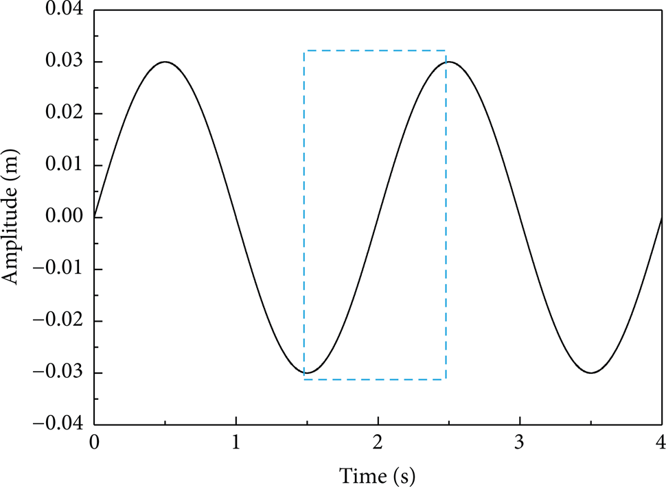
Piston displacement excitation signal.

6.2.1. Piston Velocity

Sine signal is a kind of signal related to amplitude and frequency, which is expressed in (12). The different piston velocities are gotten by changing the frequency of excitation signal. Consider

\begin{matrix} x = A \sin (2 π f t + φ) \\ \dot{x} = 2 π f A \sin (2 π f t + φ), \end{matrix}

(12)

where x is the piston displacement; $\dot{x}$ is the piston velocity; A is the amplitude; f is the frequency; t is the time; ϕ is the deviation phase angle.

The damping of Afr branch is set smaller than the other two branches. Keeping the parameter of valves and accumulators unchanged, the frequency changes are as shown in Figure 18.

Figure 18:

Frequency change of excitation signal on piston displacement.

The frequency and corresponding time range of a complete compression stroke are shown in Table 5.

Table 5:

Frequency and corresponding time range.

f (Hz)	0.1	0.25	0.5	1	1.67	2	2.5	3

t (s)	7.5∼12.5	3∼5	1.5∼2.5	0.75∼1.25	0.449∼0.749	0.375∼0.625	0.3∼0.5	0.25∼0.417

By simulation, the damping power curves under changed frequency are shown in Figure 19.

Figure 19:

Damping power characteristics responding to frequency.

In Figure 19, there are three curves in every figure. The black and red curves represent the damping power curves of A1r, A2r branch, respectively. The blue curve represents the damping power curve of Afr branch. Because the parameter settings of A1r and A2r are the same, the damping power curves of A1r and A2r almost keep coincident. The area between curve and lateral axis represents the damping work of oil flowing through the valve. The time point is marked with green dashed line in every figure. The area on the left of the green dashed line is the damping work of lower part of the compression stroke, and area on the right is the damping work of upper part of the compression stroke. The left and right area are compared to study the DNC problem. Before that, a specific definition is given in (13), which is damping noncoincidence rate (DNCR):

η = \frac{(W_{u} - W_{l})}{W_{l}},

(13)

where W_l is the damping work of lower part of the compression stroke (the area on the right of green dashed line); W_u is the damping work of upper part of the compression stroke (the area on the left of green dashed line); η represents the damping noncoincidence rate.

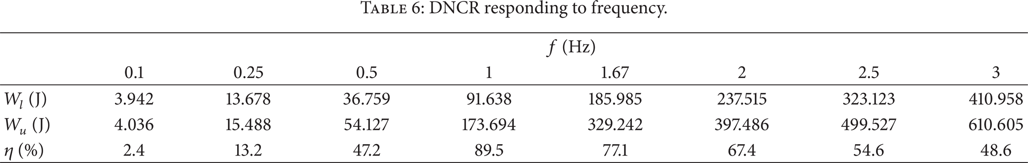
The change rule of DNCR with frequency is shown in Table 6.

Table 6:

DNCR responding to frequency.

	f (Hz)
	0.1	0.25	0.5	1	1.67	2	2.5	3

W_l (J)	3.942	13.678	36.759	91.638	185.985	237.515	323.123	410.958
W_u (J)	4.036	15.488	54.127	173.694	329.242	397.486	499.527	610.605
η (%)	2.4	13.2	47.2	89.5	77.1	67.4	54.6	48.6

Then, the variation curve of DNCR and system damping force responding to frequency is given in Figure 20.

Figure 20:

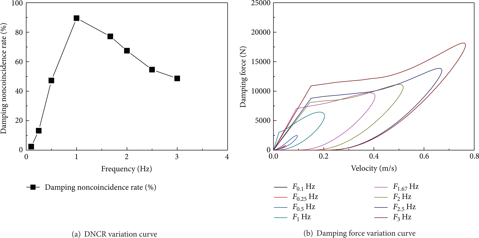
Variation curve of DNCR and damping force responding to frequency.

From Table 6 and Figure 20(a), we can see that the DNCR η first increases and then decreases. The cause can be found out in Figures 19(a)–19(h). When the frequency is low enough, the oil flowing through three branches is in the same condition. From Figure 19(a), we can see that the magnitude of damping power is very small. And the area on the left is nearly the same as the area on the right. The DNCR is only 2.4%. With the increase of piston velocity, the difference of resistance becomes bigger. Less oil flows through Afr branch because of bigger resistance. It results in the pressure of accumulator Afr being lower than the other two accumulators and out of synchronization. When the compression stroke finishes and the rebound stroke begins, a part of oil flows from accumulators A1r and A2r to Afr. The additional damping is produced in the upper half of the compression stroke, which leads to a bigger DNCR. From Table 6 we can see that the DNCR reaches the maximum around the frequency 1 Hz, resulting from the resonance of the tire, the frequency of which is around 1 Hz. With the continuous increase of piston velocity, the damping power difference between the three branches becomes narrow, which can be seen from Figures 19(e)–19(h). The DNCR decreases and levels out. The frequency range for research is chosen from 0.1∼3 Hz because higher frequency does not make sense in suspension system research. From Figure 20(b), we also can see that the damping force difference between the upper part and the lower part becomes bigger with the increase of piston frequency.

6.2.2. Parameter Setting of Valves

The damping of three branches is changed by setting diameters of throttle valves. The maximum distance h_max-r of relief valves is set as 0 mm. The diameters of throttle valves in A1r and A2r branch are kept as 7 mm, while the diameter of throttle valve in Afr branch changes as in Figure 21.

Figure 21:

Diameter change of throttle valve in Afr branch.

The frequency of the excitation signal is 2 Hz, and the time range of a complete compression stroke is 0.375 s∼0.625 s. By simulation, the damping power curves with changed diameters of throttle valve in Afr branch are shown in Figure 22.

Figure 22:

Damping power characteristics responding to throttle valve diameter.

The change rule of DNCR with throttle valve diameter is shown in Table 7.

Table 7:

DNCR responding to throttle valve diameter.

	d_t (mm)
	0	0.1	1	2	3	5	7	10	20	100

W_d (J)	313.311	309.627	260.380	252.409	239.454	202.015	161.216	120.290	94.306	90.507
W_u (J)	327.023	599.679	394.521	366.702	325.666	227.381	167.633	138.521	133.229	133.601
η (%)	4.4	64.6	51.5	45.3	36.0	12.6	4.0	15.2	41.3	47.6

Then, the variation curve of DNCR and system damping force curves responding to diameter setting of throttle valve in Afr branch are given in Figure 23.

Figure 23:

Variation curve of DNCR and damping force responding to diameter of throttle valve in Afr branch.

From Table 7 and Figure 23(a), we can see that the DNCR reaches the minimum at the diameters 0 mm and 7 mm of throttle valve Afr. As for the 7 mm condition, the damping of three branches is the same. In this condition, the DNCR reaches the minimum owing to the fact that there is no cross flow among the three branches. As for the 0 mm condition, the Afr branch is blocked. It means that the system changes to the two-branch type from the three-branch type. The DNCR also reaches the minimum since the other two branches have the same damping parameter setting. The diameters of the throttle valves in A1r and A2r branch are set as 7 mm. Setting 7 mm as standard, the greater the offset from the standard is, the bigger the DNCR is. The diameter of 0 mm is a critical condition between the three-branch and two-branch types. The closer the diameter of throttle valve in Afr branch is to 0 mm, the bigger the DNCR is. The DNCR becomes bigger and bigger and infinitely close to the vertical dashed line which goes through zero. But when the diameter of Afr throttle valve is set as 0 mm, the DNCR becomes minimum value immediately. From Figure 23(b), we also can see that the damping force difference between the upper part and the lower part is small when the diameter of Afr throttle valve becomes 0 mm and 7 mm, which is shown by the black and yellow curve. And the damping force difference becomes big with the diameter offset from the standard 7 mm.

6.2.3. Parameter Setting of Accumulators

The parameter of accumulator is changed by adjusting the precharge pressure. All the parameters of valves are set as the same. The volumes of all the accumulators are set as 1.4 L. The precharge pressure of accumulators in A1r and A2r branch is set as 35 bar. While the precharge pressure of accumulator Afr changes as in Figure 24.

Figure 24:

Precharge pressure change of accumulator in Afr branch.

The excitation signal is chosen as 2 Hz/30 mm. By simulation, the damping power curves of accumulator in Afr branch under changed precharge pressure are shown in Figure 25.

Figure 25:

Damping power characteristics responding to accumulator precharge pressure.

The change rule of DNCR to precharge pressure of accumulator is shown in Table 8.

Table 8:

DNCR responding to precharge pressure of accumulator.

	p₀ (bar)
	0	1	20	35	50	60	70	80

W_d (J)	300.414	216.319	171.858	161.229	163.311	166.244	169.371	170.361
W_u (J)	307.062	348.706	204.167	167.637	187.708	203.133	227.317	246.704
η (%)	2.2	61.2	18.8	4.0	14.9	22.2	34.2	44.8

Then, the variation curve of DNCR and system damping force responding to precharge pressure setting of accumulator in Afr branch are given in Figure 26.

Figure 26:

Variation curve of DNCR and damping force responding to precharge pressure of accumulator in Afr branch.

From Table 8 and Figure 26(a), we can see that the DNCR reaches the minimum under the precharge pressure of 0 bar and 35 bar of accumulator in Afr branch. When the precharge pressure is 35 bar, all the parameters of the three branches are the same. In this condition, the DNCR reaches the minimum owing to the fact that there is no cross flow among the three branches. As for the 0 bar condition, it means that there is no gas in the accumulator Afr. The accumulator Afr is filled with oil. The number of effective branches of the system changes from three to two. The DNCR also reaches the minimum since the other two branches have the same damping parameter setting. The precharge pressure of accumulator in A1r and A2r branch is set as 35 bar. Setting 35 bar as standard, the greater the offset from the standard is, the bigger the DNCR is. The 0 bar is a critical condition between the three-branch type and the two-branch one. The closer the precharge pressure of accumulator Afr is to 0 bar, the bigger the DNCR is. The DNCR becomes bigger and bigger and infinitely close to the vertical dashed line which goes through zero. But when the precharge pressure of accumulator in Afr branch is set as 0 bar, the DNCR decreases to minimum value immediately. From Figure 26(b), we also can see that the damping force difference between the upper part and the lower part is small when the precharge pressure of accumulator in Afr branch becomes 0 bar and 35 bar, which is shown by the black and green curve. And the damping force difference becomes big with the offset of the precharge pressure from the standard 35 bar.

Because the volume of the accumulator has the same effect as the precharge pressure of the accumulator on DNC problem, there is no need to explain it here.

7. Conclusions and Future Work

The DNC problem of IHS was proposed and described firstly in this paper. The root cause is found out according to the simulation and analysis. The main influence factors for DNC problem are studied deeply by simulation, and a quantitative comparison of DNCR was given according to the simulation results. The major findings of the study are summarized below.

As for HS with single oil line and single accumulator, the DNC problem is not significant and even does not exist.

As for IHS, owing to multiple branches and accumulators existing in the system, the DNC problem comes out and is significant. The root cause of DNC problem for IHS is the cross flow of oil among the accumulators in different branches which results from different parameters settings of every branch.

The main influence factors for DNC problem are piston velocity, valve parameter, and accumulator parameter.

Keeping all other parameters the same, with only the diameter of throttle valve in Afr branch different from that in A1r and A2r branch and a series of signals with changed frequency chosen as excitation signals, we can see that the DNCR firstly increases and then decreases as the motion frequency rises and falls. The DNCR reaches the maximum around 1 Hz which is the motion frequency of the piston.

The sine signal with fixed frequency is chosen as the excitation signal. Keeping all other parameters the same, with only the diameter of throttle valve in Afr branch varying with a series of value, we can see that The DNCR reaches the minimum when all the parameters are set as the same. The greater the offset of the diameter is, the bigger the DNCR is. The 0 mm is a critical condition in which the three-branch system changes to the two-branch type. The closer the diameter of throttle valve in Afr branch is to 0 mm, the bigger the DNCR is.

The excitation signal is also fixed. Keeping all other parameters the same, with only the precharge pressure of accumulator in Afr branch changing with a series of value, we can see that the DNCR reaches the minimum when all the parameters are set as the same. The greater the offset of the precharge pressure is, the bigger the DNCR is. The 0 bar is a critical condition in which three effective branches change to two effective branches. The closer the diameter of throttle valve in Afr branch is to 0 bar, the bigger the DNCR is. The volume of accumulator has the same effect as precharge pressure of accumulator on DNC problem.

The study of the impact of DNC problem on ride performance of vehicle and to propose a kind of effective control algorithm to reduce the negative effect is the work in the next step.

Conflict of Interests

The authors declare that there is no conflict of interests regarding the publication of this paper.

Footnotes

Acknowledgment

The project is supported by the National Science Foundation of China (Grant no. 51375046).

References

Crolla

D. A.

and King

R. P.

, “Olley's flat ride revisited,” Vehicle System Dynamics, vol. 33, pp. 762–774, 2000.

Rakheja

Wang

, and Ahmed

A. K. W.

, “Urban bus optimal passive suspension study. Phase II: enhancement of road-and driver-friendliness of urban buses through optimal suspension damping,” Transportation Canada Report T-8200-4-4556, 2001.

Cao

Rakheja

, and Su

C. Y.

, “Roll and bounce dynamic responses of heavy vehicle with interconnected suspensions,” in Proceedings of the CSME Symposium on Intelligent Vehicle and Transportation Systems, Calgary, Canada, 2006.

Liu

, An analytical study of ride and handling performance of an interconnected vehicle suspension [M.S. thesis], Concordia University, Montreal, Canada, 1994.

Wild

J. R.

Heydinger

G. J.

, and Guenther

D. A.

, “ADAMS simulation of ride and handling performance of kinetic suspension system,” SAE Paper 2006-01-1972, 2006.

Chaudhary

, Ride and roll performance analysis of a vehicle with spring loaded interconnected hydro-pneumatic suspension [M.S. thesis], Concordia University, Québec, Canada, 1998.

Lin

Zhang

, and Chen

, “Research on hydro-pneumatic balanced suspension of multi-spindled vehicle,” Applied Mechanics and Materials, vol. 66–68, pp. 855–861, 2011.

Zhang

Chen

, and Yang

, “Design and test of a hydro-pneumatic suspension with adjustable stiffness and damping,” Chinese Journal of Automotive Engineering, vol. 3, no. 2, pp. 106–112, 2013.

Chen

S.-Z.

Wang

, and Yang

, “Riding performance of a vehicle with a new type of hydro-pneumatic balanced suspension,” Transaction of Beijing Institute of Technology, vol. 29, no. 5, pp. 394–397, 2009.

10.

Cole

D. J.

, “Fundamental issues in suspension design for heavy road vehicles,” Vehicle System Dynamics, vol. 35, no. 4–5, pp. 319–360, 2001.

11.

Cebon

, Handbook of Vehicle-Road Interaction, Swets & Zeitlinger, Lisse, The Netherlands, 1999.

12.

Dudding

A. T.

and Wilson

, “Development of a new front air suspension and steer axle system for on highway commercial vehicles,” SAE Paper 2000-01-3449, 2000.

13.

Cao

, Theoretical analysis of roll and pitch coupled hydropneumatic strut suspensions [M.S. thesis], Concordia University, Québec, Canada, 2008.

14.

Cao

Song

, and Ahmadian

, “Editors' perspectives: road vehicle suspension design, dynamics, and control,” Vehicle System Dynamics, vol. 49, no. 1–2, pp. 3–28, 2011.

15.

Cao

Rakheja

, and Su

C. Y.

, “Roll plane analysis of interconnected hydro-pneumatic suspension struts,” in Proceedings of the ASME International Mechanical Engineering Congress and Exposition (IMECE '05), vol. 80484, Orlando, Fla, USA, 2005.

16.

Cao

Rakheja

, and Su

C.-Y.

, “Heavy vehicle pitch dynamics and suspension tuning. Part I: unconnected suspension,” Vehicle System Dynamics, vol. 46, no. 10, pp. 931–953, 2008.

17.

Cao

Rakheja

, and Su

C.-Y.

, “Roll- and pitch-plane coupled hydro-pneumatic suspension. Part 1: feasibility analys is and suspension properties,” Vehicle System Dynamics, vol. 48, no. 3, pp. 361–386, 2010.

18.

Cao

Rakheja

, and Su

C.-Y.

, “Roll- and pitch-plane-coupled hydro-pneumatic suspension. Part 2: dynamic response analyses,” Vehicle System Dynamics, vol. 48, no. 4, pp. 507–528, 2010.

19.

Zhang

Smith

W. A.

, and Jeyakumaran

, “Hydraulically interconnected vehicle suspension: background and modelling,” Vehicle System Dynamics, vol. 48, no. 1, pp. 17–40, 2010.

20.

Zhang

Wang

, and Du

, “Motion-mode energy method for vehicle dynamics analysis and control,” Vehicle System Dynamics, vol. 52, no. 1, pp. 1–25, 2014.

21.

Zhang

, and Wang

, “Switched control of vehicle suspension based on motion-mode detection,” Vehicle System Dynamics, vol. 52, no. 1, pp. 142–165, 2014.

22.

Ding

Han

Luo

, and Zhang

, “Modelling and characteristic analysis of tri-Axle trucks with hydraulically interconnected suspensions,” Vehicle System Dynamics, vol. 50, no. 12, pp. 1877–1904, 2012.

23.

Smith

W. A.

Zhang

, and Jeyakumaran

, “Hydraulically interconnected vehicle suspension: theoretical and experimental ride analysis,” Vehicle System Dynamics, vol. 48, no. 1, pp. 41–64, 2010.

24.

, Research on system dynamics simulation and test of hydro-pneumatic suspension [M.S. thesis], Zhejiang University, 2000.

25.

Yoshimura

and Emoto

, “Steering and suspension system of a full car model using fuzzy reasoning based on single input rule modules,” International Journal of Vehicle Autonomous Systems, vol. 1, no. 2, pp. 237–255, 2003.

26.

Yang

Chen

Zhao

, and Yang

, “Design and testing on the hydro-pneumatic suspensions with controllable stiffness and damping,” Transactions of the Chinese Society of Agricultural Machinery, vol. 39, no. 10, pp. 6–24, 2008.

27.

Yang

, Research on adjustable damping technology based on hydro-pneumatic suspensions [Ph.D. dissertation], Beijing Institute of Technology, 2010.

28.

Zhao

, Research on nonlinearity and damping control strategy of hydro-pneumatic suspension [Ph.D. dissertation], Beijing Institute of Technology, 2011.

29.

Zhao

Y.-Z.

and Chen

S.-Z.

, “Investigation of sliding mode control for semi-active hydro-pneumatic suspension based on a full vehicle model,” Transaction of Beijing Institute of Technology, vol. 31, no. 10, pp. 1168–1173, 2011.

30.

Wang

and Chen

S.-Z.

, “External characteristics design of adjustable damping valve of hydro-pneumatic balanced suspension for vehicles,” Transaction of Beijing Institute of Technology, vol. 32, no. 12, pp. 1235–1240, 2012.

Research on Damping Noncoincidence and Its Influence Factors of Multibranch Hydropneumatic Suspension

Abstract

1. Introduction

2. Description of IHS System

3. Statement of DNC Problem

4. Multibranch HS System Model

4.1. Model of Accumulator

4.2. Model of Throttle Valve

4.3. Model of Check Valve and Relief Valve

4.4. Model of Suspension System

5. The Root Cause of DNC Problem

6. Influence Factors of DNC Problem

6.1. Statement of Influence Factors

6.2. Simulation Analysis of Influence Factors

6.2.1. Piston Velocity

6.2.2. Parameter Setting of Valves

6.2.3. Parameter Setting of Accumulators

7. Conclusions and Future Work

Conflict of Interests

Footnotes

Acknowledgment

References