
Abstract
The variability of specific heats, internal irreversibility, heat and frictional losses are neglected in air-standard analysis for different internal combustion engine cycles. In this paper, the performance of an air-standard Diesel cycle with considerations of internal irreversibility described by using the compression and expansion efficiencies, variable specific heats, and losses due to heat transfer and friction is investigated by using finite-time thermodynamics. Artificial neural network (ANN) is proposed for predicting the thermal efficiency and power output values versus the minimum and the maximum temperatures of the cycle and also the compression ratio. Results show that the first-law efficiency and the output power reach their maximum at a critical compression ratio for specific fixed parameters. The first-law efficiency increases as the heat leakage decreases; however the heat leakage has no direct effect on the output power. The results also show that irreversibilities have depressing effects on the performance of the cycle. Finally, a comparison between the results of the thermodynamic analysis and the ANN prediction shows a maximum difference of 0.181% and 0.194% in estimating the thermal efficiency and the output power. The obtained results in this paper can be useful for evaluating and improving the performance of practical Diesel engines.
1. Introduction
The cycle experienced in the cylinder of an internal combustion engine is very complex; to make the analysis of an engine cycle much more manageable, the real cycle is approximated with an ideal air-standard cycle, which differs from the actual one by some aspects. Variable specific heat of the working fluid, internal irreversibility, heat transfer through the cylinder wall, and friction are factors that affect the engine performance, whereas they are neglected in dealing with thermodynamic analysis of ideal air-standard cycles. The Diesel cycle is the ideal air-standard cycle for CI reciprocating engines. The CI engine, first proposed by Rudolph Diesel in the 1890s, is very similar to the SI engine, differing mainly in the method of initiating combustion [1–3]. In recent years, several attentions have been paid to the performance of internal combustion engines for different cycles. Effects of friction and temperature-dependent specific heat of the working fluid on the performance of a Diesel engine have been performed by Al-Sarkhi et al. [4]. Performance analysis of air-standard Diesel cycle using an alternative irreversible heat transfer approach has been investigated by Al-Hinti et al. [5]. Reciprocating heat-engine cycles have been done by Ge et al. [6]. Power, efficiency, entropy-generation rate, and ecological optimization for a class of generalized irreversible universal heat-engine cycles have been studied by Chen et al. [7]. Heat loss as a percentage of fuels energy in air-standard Otto and Diesel cycles has been performed by Ozsoysal [8]. Comparative performance analysis of irreversible Dual and Diesel cycles under maximum power conditions has been investigated by Parlak [9]. Second-law analyses applied to internal combustion engines operation have been presented by Rakopoulos and Giakoumis [10]. Energy, exergy, and second-law performance criteria have been studied by Lior and Zhang [11]. Thermodynamic irreversibilities and exergy balance in combustion processes have been reported by Som and Datta [12]. Second-law analysis of an ideal Otto cycle has been performed by Lior and Rudy [13]. First- and second-law analysis of an ejector expansion Joule-Thomson cryogenic refrigeration cycle and first- and second-laws analysis of an air-standard Dual cycle with heat loss consideration have been investigated by Rashidi et al. [14, 15]. Finite-time thermodynamic modelling and analysis of an irreversible Otto and Dual cycles have been studied by Ge et al. [16, 17]. Performance analysis of a Diesel cycle under the restriction of maximum cycle temperature with considerations of heat loss, friction, and variable specific heats has been done by Hou and Lin [18] and correct evaluation of effects of heat transfer on the exergy efficiency of an air-standard Otto cycle has been performed by Rashidi et al. [19]. During recent decades, some different studies have been performed about the applications of AI (artificial intelligence) methods, especially ANN (artificial neural network), in thermodynamics. Kalogirou [20] applied AL techniques to model and predict the performance and the control of combustion process. Furthermore, Deh Kiani et al. [21] have presented a paper about ANN modeling of a spark ignition engine for predicting the engine brake power, output torque, and exhaust emissions of the engine. In addition, Gandhidasan and Mohandes [22] have proposed the application of ANN-based model for simulation of the relationship between the inlet and outlet parameters of a dehumidifier. They applied a multilayer ANN for dehumidifier performance investigation. Moreover, some ANN models have been presented in order to predict the fresh steam properties from a brown coal-fired boiler of a power plant by Smrekar et al. [23] using real plant data. Rashidi et al. [24] illustrated the parametric analysis and optimization of entropy generation in unsteady MHD flow past a stretching rotating disk using artificial neural network (ANN) and particle swarm optimization (PSO) algorithm. In another study, Rashidi et al. [25] performed the parametric study and optimization of regenerative Clausius and organic Rankine cycles with two feedwater heaters. They proposed a procedure based on the combination of ANN and artificial bees colony (ABC). They have selected thermal efficiency, exergy efficiency, and specific work as the objective functions of optimization and have evaluated the mentioned parameters for different values of the outlet pressures from the second and third pumps and finally Rashidi et al. [26], using artificial neural networks and genetic algorithms, analyzed and optimized a transcritical power cycle with regenerator.
In this study, the effects of various parameters of irreversibility such as internal irreversibility (compression and expansion efficiencies), variable specific heats of the working fluid, heat loss, and friction on the first-law and the second-law efficiency of Diesel cycle are investigated. In addition to that, ANN is employed to predict the thermal efficiency and power output values of the considered Diesel cycle versus the minimum and maximum temperatures as well as the compression ratio.
2. Thermodynamic Analysis
2.1. First-Law Efficiency Analysis
Since thermodynamic analysis of internal combustion engines in practical conditions is extremely complex, for this reason the real cycles are approximated with ideal air-standard cycles by applying a number of assumptions. The T-s diagram for an air-standard Diesel cycle is shown in Figure 1. It can be seen that the compression processes (1 → 2s) and (1 → 2) are reversible and irreversible adiabatic processes, respectively. The heat addition process (2 → 3) is an isobaric process; the expansion processes (3 → 4s) and (3 → 4) are reversible and irreversible adiabatic processes, respectively. The cycle is completed by an isochoric heat rejection process (4 → 1). In the air-standard analysis, the working fluid is assumed to behave as an ideal gas with constant specific heats. But, this assumption can be valid only for the small temperature ranges during the cycle. For the large temperature range of 300 → 2000 K, this assumption cannot be applied, because it causes considerable errors. Hence, with a suitable approximation, the specific heats of the working fluid can be written as linear functions of temperature [16]:

where a p , b v , and k1 are constants and C p and C v are the specific heats at constant pressure and constant volume, respectively. Due to the relation between the specific heats, one can obtain the working fluid gas constant as [4]

As it can be seen in Figure 1, in the ideal air-standard Diesel cycle, for the reversible adiabatic compression (1 → 2s) and expansion (3 → 4s) processes, the entropy generation and thus the entropy change of the working fluid are zero, while as in a real Diesel cycle, the irreversibilities cause the entropy of the working fluid to increase, during the irreversible adiabatic compression (1 → 2) and expansion (3 → 4) processes. Therefore, the following compression and expansion efficiencies can be used to describe the internal irreversibilities of the compression and expansion processes, respectively, [19]


The heat added per second in the isobaric heat addition process (2 → 3) may be written as

The heat rejected per second in the isochoric heat-rejection process (4→1) may be written as

where M is the mass of the working fluid and N is cycles per second.

The T-s diagram for an air-standard Diesel cycle.
The entropy changes for a reversible process (i → j) as follows:

Plug (3) for C v into (7), for the compression and expansion isentropic processes, we have

where the compression ratio, r c , and the cutoff ratio, r, are defined as

On the other hand, according to (3) and (4), for T2 and T4, we have

The temperatures within the combustion chamber of an internal combustion engine can reach about 2700 (K) and above. Materials in the engine cannot tolerate this kind of high temperature and would quickly fail if proper heat transfer does not occur. Therefore to protect the engine from thermal failure, the interior maximum temperature of the combustion chamber must be limited to much lower values by heat fluxes through the cylinder wall during the combustion period. Since during the other processes of the operating cycle, the heat flux is essentially quite small and negligible due to the very short time involved for the processes, it is assumed that the heat loss through the cylinder wall occurs only during combustion. The calculation of actual heat transfer through the cylinder wall occurring during combustion is complex. It is customary therefore to approximate cylinder wall heat transfer flux as being proportional to the average temperature of both the working fluid and cylinder wall, T0. Furthermore automobile engineers generally assume that, during the operation, the wall temperature remains approximately invariant. The heat released by combustion per second can be obtained as [16]
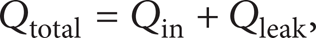
where Qin is obtained from (5) and Qleak can be defined as [17]

where, T0 is the average temperature of the cylinder wall, β1 is the thermal conductivity between the working fluid and the cylinder wall, and β is the constant related to heat transfer, where β = β1/2·
For the Diesel cycle and assuming a dissipation term represented by a friction force which is a linear function of the velocity gives [17]

where μ is a coefficient of friction, which takes into account the global losses and x is the piston position. Then, the lost power is

If one specifies the engine to be a four-stroke cycle engine, then the total distance the piston travels per cycle is

where x1 and x2 are the piston positions at maximum and minimum volumes, respectively.
For a four-stroke cycle engine, running at N cycles per second, the mean velocity of the piston is
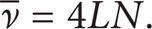
According to above description, the power output is

Finally, the first-law efficiency (thermal efficiency) is

2.2. Second-Law Efficiency Analysis
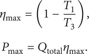
The second-law analysis is a good benchmark for the availability of systems that is described as the ratio of the actual thermal efficiency (first-law efficiency) to the maximum possible (reversible) thermal efficiency under the same conditions. For the work-producing devices, the second-law efficiency can also be expressed as the ratio of the useful power output to the maximum possible (reversible) power output [1, 3]. According to the above description, the second-law efficiency of an air-standard Diesel cycle is defined as

where ηmax and Pmax are the maximum possible efficiency (the Carnot efficiency) and the maximum possible power output of the Diesel cycle, respectively, that are defined as follows:
3. Prediction of Thermal Efficiency and Power Output Using Artificial Neural Network
3.1. Artificial Neural Network Theory
The artificial neural networks (ANNs) are a different paradigm for computing. ANNs are based on a parallel architecture to animal brains. They are a form of a multiprocessor computer system by simple scalar messages, simple processing elements, and a high degree of interconnection and adoptive interaction between elements. Multilayer feed forward (MLFF) is the most popular type of ANNs. A diagram of a MLFF neural network is demonstrated in Figure 2. The network includes usually an input layer, some hidden layers, and an output layer. Meanwhile the knowledge is usually stored in connection weights. The process of modifying the connection weights using a suitable learning method is called training:
The most widely used learning algorithm of MLFF neural networks is the BEP, a method proposed by McClelland et al. (1987) [27] in a ground-breaking study focused on cognitive computer science.
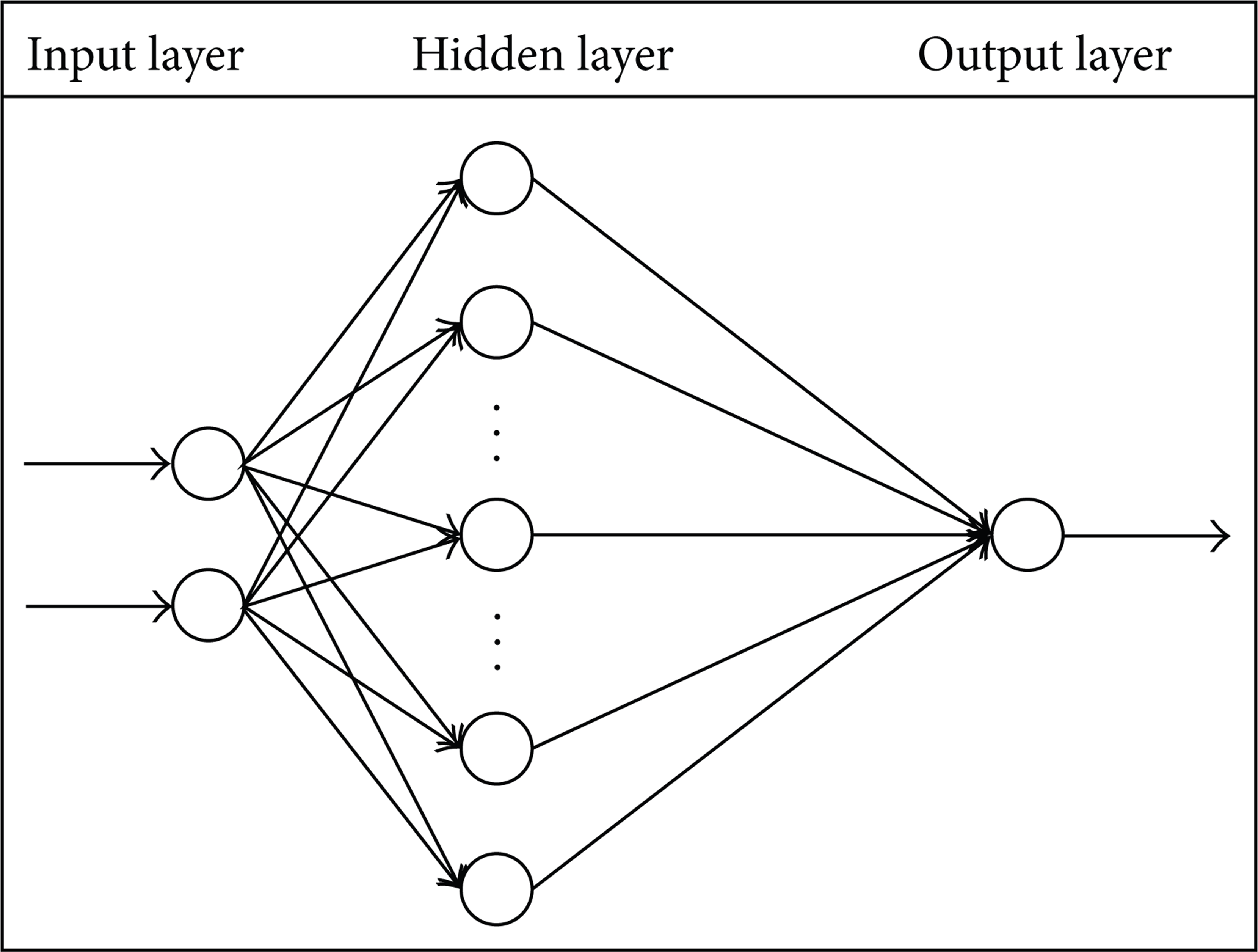
A diagram of a MLFF neural network.
In this paper, the structure of the ANNs consists of three layers, that is, the input, hidden, and output layers. The magnitudes of ω ab are the weights between the input and the hidden layers and those of ω bc are the weights between the hidden and the output layer. The operation of the BEP method consists of three stages:
feed-forward stage:

where o is the output, τ the input, y the output of hidden layer, and ϕ the activation function,
back-propagation stage:

where δ is the local gradient function, e shows the error function, and o and d are the actual and desired outputs, respectively,
adjustable weighted value stage:

where ζ is the learning rate. Repeating these 3 stages led to a value of the error function, which will be zero or a constant value.
3.2. Prediction Using Artificial Neural Network
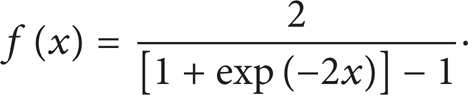
The thermal efficiency and power output prediction parts of this study consist of three steps. First of all a MLFF neural network is created with input, hidden, and output layers, with 2, 10, and 1 neurons, respectively, for each of procedures. The transfer functions for the neurons of hidden and output layers are tansig, defined in (21). The inputs of the ANNs are T min , Tmax, and r c , and the target outputs are thermal efficiency and power output. In the next step, the train of ANN is done based on the data of 1600 different conditions using the BEP method. In the training procedure of ANN, the BEP iterations are assumed to be 500. In the BEP training procedure 70%, 20%, and 10% of data are used for training, testing, and verification of neural network, respectively. The training procedures using BEP are shown in Figure 3. As it can be seen, the training procedures have been done with good approximations. In the third step, the trained ANNs are used to predict the thermal efficiency and power output values of conditions which had not been used in the training procedure. The obtained results are also compared with the finite-time thermodynamics results.

Training procedures of interpolation part using BEP with respect to (a) minimum temperature and compression ratio for power output; (b) minimum temperature and compression ratio for thermal efficiency; (c) maximum temperature and compression ratio for power output; (d) maximum temperature and compression ratio for thermal efficiency.
4. Results and Discussion
Following [4], the parameters selected for numerical analysis are shown in Table 1. Substituting the parameters and constants of Table 1 into the obtained equations, we can get ranges of temperature of different states, the heat added, the power output, the maximum passible power output, the first-law efficiency, the maximum passible thermal efficiency, and the second-law efficiency in the specified range.
Thermodynamic parameters used in this paper.

Figures 4, 5, 6, 7, 8, 9, 10, 11, 12, 13, 14, 15, 16, 17, 18, 19, 20, 21, 22, 23, 24, 25, 26, 27, 28, 29, 30, and 31 present selected computations for the effects of the key thermodynamic parameters. When T1 and T3 are given, T2s and T4s can be readily obtained via (8); T2 and T4 are obtained from (10). Figures 4–10 illustrate the effects of parameters T min , Tmax, η c , η e , β, a p , b v , k1, and μ on the first-law efficiency of the cycle for different values of the compression ratio. It can be seen that the first-law efficiency increases with increasing compression ratio, reaches a maximum value, and then decreases, for fixed value of each one of these parameters. These figures also show that, for r c < 10, the first-law efficiency increases as T min increases and Tmax decreases. For r c > 10, the efficiency increases as T min decreases and as Tmax increases. The compression and expansion efficiencies are between 0.96 and 1. When these efficiencies are close to 1, the first-law efficiency will increase and vice versa. The first-law efficiency increases as β decreases which is related to heat loss. For r c < 13, the first-law efficiency increases as the invariable parts of the specific heat a p and b v decrease; however, for r c > 13, it increases as both of them increase. It is noticed that for r c < 12 or r c > 12 the effect of decreasing or increasing k1, respectively, will increase the first-law efficiency. As it is expected, reducing the friction parameter μ will enhance the first-law efficiency.
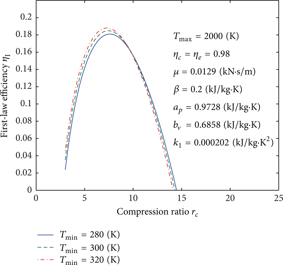
Influence of T min on curves of the first-law efficiency versus the compression ratio.

Influence of Tmax on curves of the first-law efficiency versus the compression ratio.

Influence of η c and η e on curves of the first-law efficiency versus the compression ratio.

Influence of β on curves of the first-law efficiency versus the compression ratio.
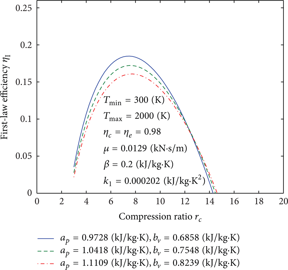
Influence of a p and b v on curves of the first-law efficiency versus the compression ratio.
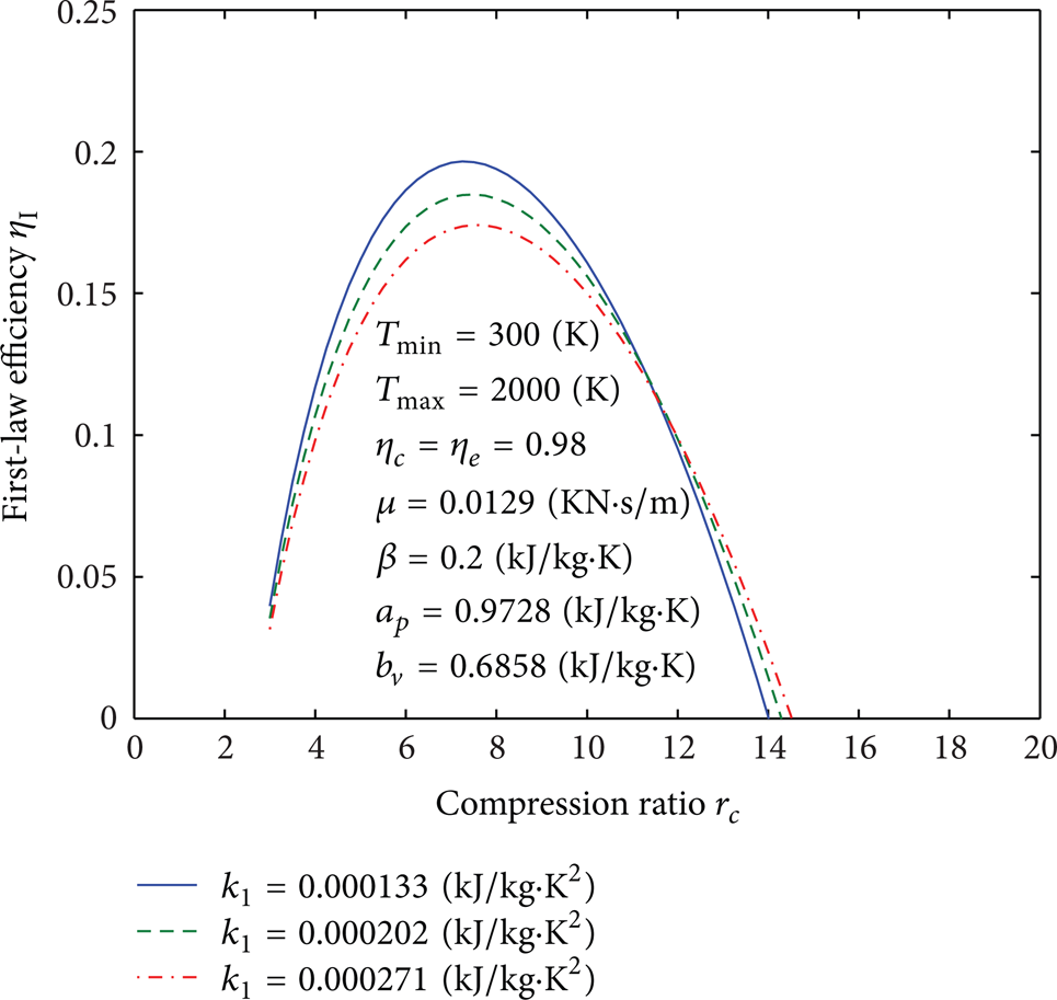
Influence of k1 on curves of the first-law efficiency versus the compression ratio.

Influence of μ on curves of the first-law efficiency versus the compression ratio.

Influence of T min on curves of the power output versus the compression ratio.

Influence of Tmax on curves of the power output versus the compression ratio.

Influence of η c and η e on curves of the power output versus the compression ratio.

Influence of β on curves of the power output versus the compression ratio.

Influence of a p and b v on curves of the power output versus the compression ratio.

Influence of k1 on curves of the power output versus the compression ratio.

Influence of μ on curves of the power output versus the compression ratio.

Influence of T min on curves of the power output versus the first-law efficiency.

Influence of Tmax on curves of the power output versus the first-law efficiency.

Influence of η c and η e on curves of the power output versus the first-law efficiency.

Influence of β on curves of the power output versus the first-law efficiency.

Influence of a p and b v on curves of the power output versus the first-law efficiency.

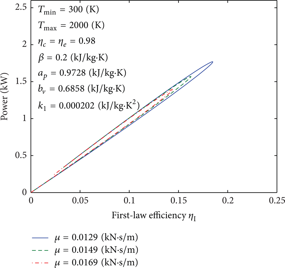
Influence of k1 on curves of the power output versus the first-law efficiency.
Influence of μ on curves of the second-law efficiency versus the first-law efficiency.

Influence of T min on curves of the second-law efficiency versus the first-law efficiency.

Influence of Tmax on curves of the second-law efficiency versus the first-law efficiency.
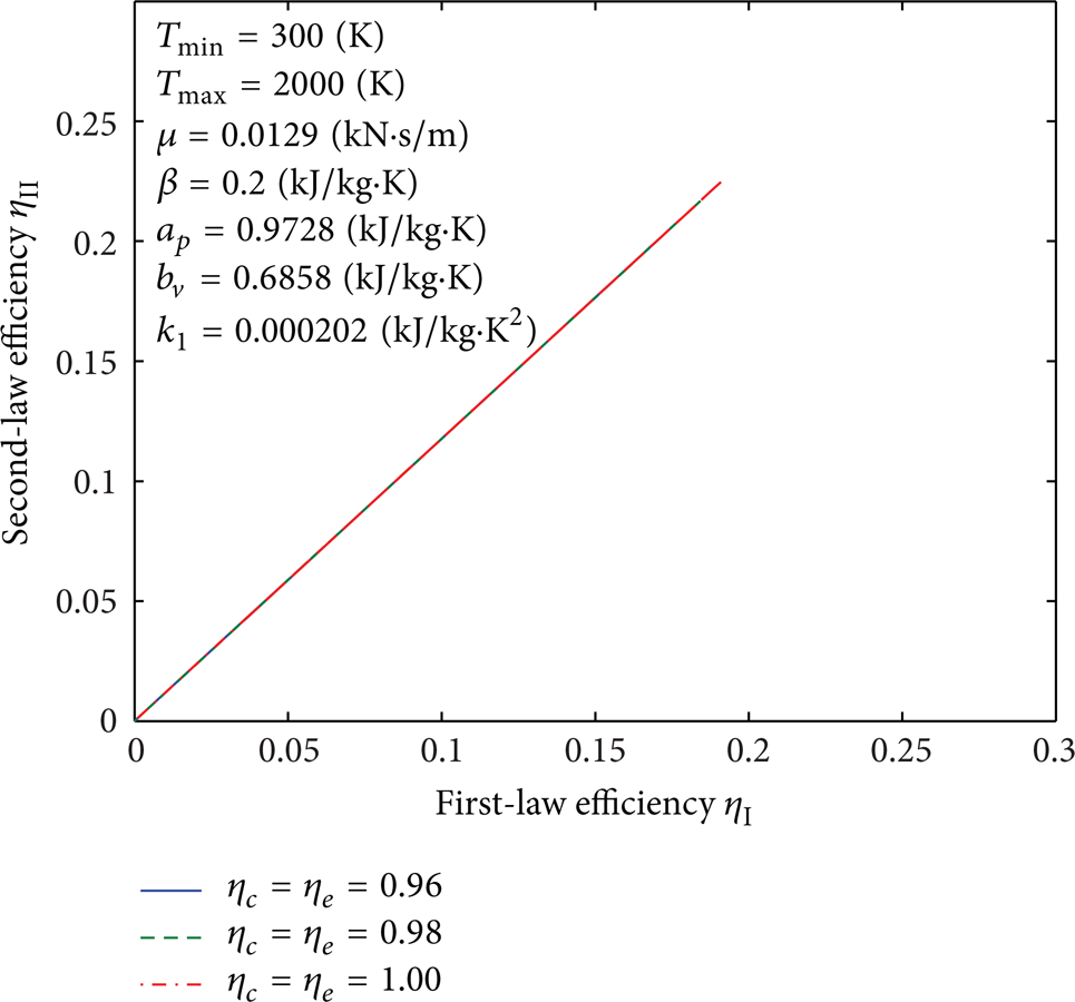
Influence of η c and η e on curves of the second-law efficiency versus the first-law efficiency.

Influence of β on curves of the second-law efficiency versus the first-law efficiency.

Influence of a p and b v on curves of the second-law efficiency versus the first-law efficiency.

Influence of k1 on curves of the second-law efficiency versus the first-law efficiency.

Influence of μ on curves of the second-law efficiency versus the first-law efficiency.
Figures 11–17 show effects of parameters T min , Tmax, η c , η e , β, a p , b v , k1, and μ on the power output of the cycle for different values of the compression ratio. It can be seen that the output power increases with increasing compression ratio, reaches a maximum value, and then decreases, for fixed value of each one of these parameters. For r c < 7, the power output increases as T min increases and Tmax decreases; and for r c > 7, the power output increases as T min decreases and Tmax increases. When the compression and expansion efficiencies increase, the power output decreases and vice versa. Based on (12) and (17), parameter β has no direct effect on the power output. For r c < 9, the power output increases as a p and b v , that are invariable parts of specific heat, decrease; and for r c > 9, the power output increases as increase of them. For r c < 7 or r c > 7 the effect of decreasing or increasing k1, respectively, will increase the power output. Similarly, reducing the friction parameter μ will enhance the power output.
Figures 18–24 indicate the influence of parameters T min , Tmax, η c , η e , β, a p , b v , k1, and μ on the power output versus the first-law efficiency, which have a loop shape. The maximum value of the power output corresponds to the maximum value of the first-law efficiency. The first-law efficiency and the power output increase as μ, η c , and η e decrease. For fixed value of the power output, the first-law efficiency increases as T min increases and Tmax, β, a p , b v , and k1 decrease.
Figures 25–31 illustrate effects of the parameters T min , Tmax, η c , η e , β, a p , b v , k1, and μ on the second-law efficiency versus the first-law efficiency. Recall Figures 4–10; the first-law efficiency has the same value at two different compression ratios before it reaches its maximum. With this description in mind, Figures 25–31 indicate that the larger second-law efficiency occurs at the smaller compression ratio. In addition, it can be seen that the first-law and the second-law efficiencies increase as η c and η e increase and β, a p , b v , k1, and μ decrease. For fixed value of the first-law efficiency, the second-law efficiency increases as T min increases and Tmax decreases.
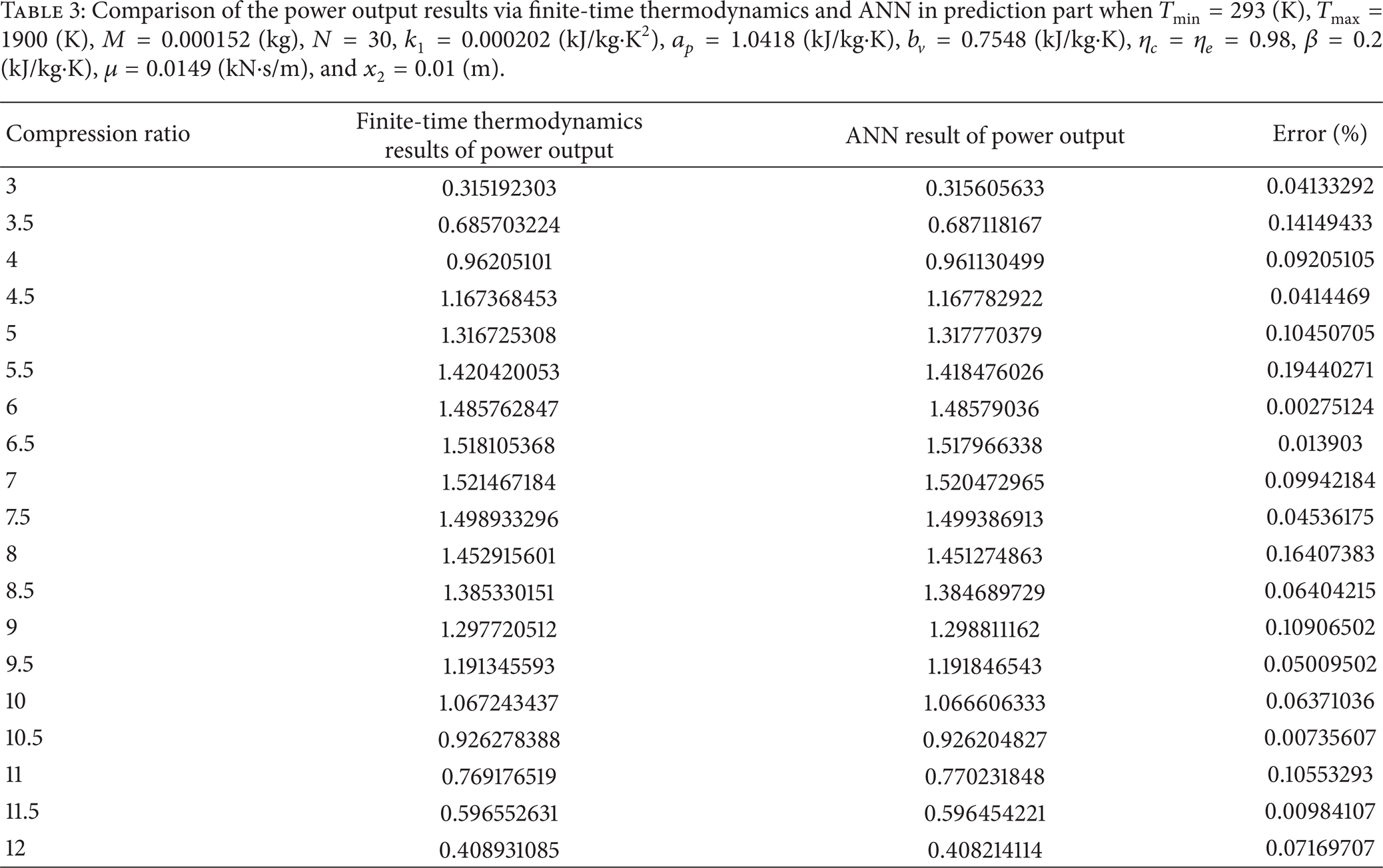
In the prediction part of this study, Tables 2 and 3 show a comparison of the obtained thermal efficiency (first-law efficiency) and power output via ANN and finite-time thermodynamics for different values of compression ratio. As can be seen in these tables, there is an excellent correlation between finite-time thermodynamics and ANN predicted data. So it can be concluded that the proposed procedure based on ANN can be used to interpolate the thermal efficiency and power output values for different conditions. The minimum, maximum, and average value of errors which are defined based on the difference between ANN and finite-time thermodynamics results are 0.0021353%, 0.18105927%, and 0.041549636%, respectively, for thermal efficiency and 0.00275124%, 0.194402708%, and 0.074846647%, respectively, for power output.
Comparison of the thermal efficiency results via finite-time thermodynamics and ANN in prediction part when T min = 293 (K), Tmax = 1900 (K), M = 0.000152 (kg), N = 30, k1 = 0.000202 (kJ/kg·K2), a p = 1.0418 (kJ/kg·K), b v = 0.7548 (kJ/kg·K), η c = η e = 0.98, β = 0.2 (kJ/kg·K), μ = 0.0149 (kN·s/m), and x2 = 0.01 (m).

Comparison of the power output results via finite-time thermodynamics and ANN in prediction part when T min = 293 (K), Tmax = 1900 (K), M = 0.000152 (kg), N = 30, k1 = 0.000202 (kJ/kg·K2), a p = 1.0418 (kJ/kg·K), b v = 0.7548 (kJ/kg·K), η c = η e = 0.98, β = 0.2 (kJ/kg·K), μ = 0.0149 (kN·s/m), and x2 = 0.01 (m).
In another investigation, the ANNs, that were trained before, are used to plot the 3D continuous layers of thermal efficiency and power output against the maximum and minimum temperatures and compression ratio. Figures 32 and 33 present these layers. The trained ANN can be applied to predict data in points that finite-time thermodynamics data are not available there. Therefore, some data in addition to finite-time thermodynamics data are obtained and then are used to plotting layers. So the layers have been plotted more accurately. Figures 34 and 35 show comparisons [18] of the first-law efficiency versus compression ratio and the output power versus the first-law efficiency, respectively. This comparison shows a good agreement between the current results and those of [18] for the same internal values and constants. Therefore it gives confidence about our results.

3D continuous layer of power output against maximum temperature and compression ratio when T min = 300 (K), M = 0.000152 (kg), N = 30, k1 = 0.000202 (kJ/kg·K2), a p = 1.0418 (kJ/kg·K), b v = 0.7548 (kJ/kg·K), η c = η e = 0.98, β = 0.2 (kJ/kg·K), μ = 0.0149 (kN·s/m), and x2 = 0.01 (m).

3D continuous layer of thermal efficiency against minimum temperature and compression ratio when Tmax = 1900 (K), M = 0.000152 (kg), N = 30, k1 = 0.000202 (kJ/kg·K2), a p = 1.0418 (kJ/kg·K), b v = 0.7548 (kJ/kg·K), η c = η e = 0.98, β = 0.2 (kJ/kg·K), μ = 0.0149 (kN·s/m), and x2 = 0.01 (m).

A verification compared to [18] (the first-law efficiency versus the compression ratio).

A verification compared to [18] (the power output versus the first-law efficiency).
5. Conclusions
In this paper, the performance of an air-standard Diesel cycle with consideration of internal irreversibility, variable specific heats of the working fluid, losses due to heat transfer, and friction has been analyzed and the effects of different factors on the first-law efficiency, the power output, and the second-law efficiency have been reported. The obtained results show that the effects of irreversibilities on the performance of the Diesel cycle are obvious and should be considered in practical Diesel cycle analysis. Based on this analysis, the irreversibilities cause strong effects on the performance of the cycle. Meanwhile in this study a procedure has been proposed for prediction of thermal efficiency and power output values using ANN. The comparison of finite-time thermodynamics and ANN results displays that the proposed procedure can be applied to predict the thermal efficiency and power output values for different conditions where the finite-time thermodynamics analysis has not been performed with good correlations.
Footnotes
Nomenclature
Conflict of Interests
The authors declare that they have no conflicts of interests.
Acknowledgment
The authors extend their appreciation to the Deanship of Scientific Research at King Saud University for funding this work through the research group Project no. RGP-VPP-080.