Sage Journals: Discover world-class research

Abstract

The large eddy simulation (LES) of spatially evolving supersonic boundary layer transition over a flat-plate with freestream Mach number 4.5 is performed in the present work. The Favre-filtered Navier-Stokes equations are used to simulate large scales, while a dynamic mixed subgrid-scale (SGS) model is used to simulate subgrid stress. The convective terms are discretized with a fifth-order upwind compact difference scheme, while a sixth-order symmetric compact difference scheme is employed for the diffusive terms. The basic mean flow is obtained from the similarity solution of the compressible laminar boundary layer. In order to ensure the transition from the initial laminar flow to fully developed turbulence, a pair of oblique first-mode perturbation is imposed on the inflow boundary. The whole process of the spatial transition is obtained from the simulation. Through the space-time average, the variations of typical statistical quantities are analyzed. It is found that the distributions of turbulent Mach number, root-mean-square (rms) fluctuation quantities, and Reynolds stresses along the wall-normal direction at different streamwise locations exhibit self-similarity in fully developed turbulent region. Finally, the onset and development of large-scale coherent structures through the transition process are depicted.

1. Introduction

The development of the super/hypersonic aircraft has been one of the cutting edges in aerospace technology in recent years. As a key fundamental problem faced by the mission, the compressible boundary layer transition is a challenging problem. Boundary layer transition has a significant impact on the performances of the super/hypersonic aircraft including the vehicle aerodynamics, aerothermodynamics, inlet performances, and the mixing efficiency of the combustion chamber. It would thus have important engineering significance on understanding the mechanisms of the transition as well as accurately predicting and controlling the transition. Along with the continuous improvement on computational fluid dynamics and the rapid development of computer technology, numerical simulation has been widely applied to the fundamental research and engineering design for fluid mechanics. In current study on the mechanism of supersonic boundary layer transition, direct numerical simulation (DNS) and large eddy simulation (LES) methods play an important role.

Dinavahi et al. [1] performed a temporal DNS of boundary layer transition flow around a cone with freestream Mach number Ma_∞ = 4.5. A temporal subharmonic transition in a Ma_∞ = 4.5 flat-plate boundary layer has been simulated successfully by Adams and Kleiser [2] using DNS. Guarini et al. [3] carried out a temporal DNS of an adiabatic supersonic turbulent boundary layer whose Mach number is equal to Ma_∞ = 2.5. Maeder et al. [4] performed a DNS of a turbulent supersonic boundary layer at various Mach numbers (Ma_∞ = 3, 4.5, and 6) using an extended temporal DNS approach, which is based on the assumption of slow growth of the boundary layer. Their results showed that compressibility effects on turbulence statistics are small up to Mach number of about 5. Pirozzoli et al. [5] performed a DNS of a spatially evolving supersonic adiabatic flat-plate boundary layer flow at Ma_∞ = 2.25 to assess the validity of Morkovin's hypothesis and Reynolds analogies and to analyze the controlling mechanisms for turbulence production, dissipation, and transport. Huang et al. [6] and Cao et al. [7] performed simulations of a flat-plate boundary layer flow at Ma_∞ = 4.5 using temporal and spatial DNS, respectively. They found that the mechanism causing the mean flow profile to evolve swiftly from laminar to turbulent was the modification of mean flow profile by the disturbance. Li et al. [8] and Liang and Li [9] performed DNS of a spatially developing hypersonic flat-plate boundary layer flow at Ma_∞ = 6 and 8, respectively.

El-Hady and Zang [10] investigated the LES of the boundary layer transition around a cylinder with Ma_∞ = 4.5 by temporal approach. The results showed that the Λ vortex structures in the early stages of transition can be captured even with coarse mesh. Shan et al. [11] proposed an LES of a spatially evolving flat-plate boundary layer flow at Ma_∞ = 4.5 and obtained the whole process of transition. Stolz et al. [12] performed an LES study on the supersonic boundary layer transition under the same conditions of Adams and Kleiser [2]. The results demonstrated that the LES results were consistent with the DNS, but the amount of computation was two orders of magnitude smaller than the DNS. Pan et al. [13, 14] performed LES of boundary layer transition over a supersonic flat-plate and a hypersonic blunt-wedge, respectively. In addition, the LES of compressible transition flows with engineering background has also made some progress [15 –17].

Because of the numerical difficulty, most DNS of transition are limited to temporal mode, in which streamwise periodic boundary condition is imposed. Compared to the temporal mode, the spatial mode does not need any artificial assumption and seems more reliable. As can be seen, LES has been successfully applied to the numerical simulation of supersonic boundary layer transition and plays an active role in studying the mechanism of transition. Meanwhile, the total number of grids required for LES is one to two orders of magnitude less than DNS; thus the amount of computation for LES is significantly less than DNS, indicating that LES is capable of solving problems with complex geometry using spatial approach. Therefore, LES is the most potential method for the numerical simulation of spatially developing supersonic boundary layer transition under the capacity of modern computers.

In this study, a spatial LES of a supersonic flat-plate boundary layer flow at Ma_∞ = 4.5 is analyzed. The study is intended to confirm the LES method established in the present work and provide additional information on the supersonic transitional flowfield that can only be accomplished through a spatial simulation. The variations of typical statistical quantities in the transition process are analyzed, and some characteristics of fully developed turbulence are investigated. The onset and development of Λ vortices, hairpin vortices, ring-like vortices, and the broken of ring-like vortices are also depicted.

2. Numerical Method

Three-dimensional, unsteady compressible Favre-filtered Navier-Stokes equations, whose filtered energy equation is represented in terms of Vreman's resolved total energy [18], are solved numerically. The residual subgrid stress, defined as $τ_{i j} = - \bar{ρ} (\tilde{u_{i} u_{j}} - {\tilde{u}}_{i} {\tilde{u}}_{j})$ , is modeled using the dynamic mixed subgrid-scale (SGS) model, which is validated by a simulation of turbulent channel flow [19] as

\begin{matrix} τ_{i j} - \frac{1}{3} τ_{k k} δ_{i j} = 2 {C Δ}^{2} \bar{ρ} | \tilde{S} | ({\tilde{S}}_{i j} - \frac{1}{3} {\tilde{S}}_{m m} δ_{i j}) + L_{i j}^{m} - \frac{1}{3} L_{k k}^{m} δ_{i j}, \\ τ_{k k} = - 2 C_{I} Δ^{2} \bar{ρ} {| \tilde{S} |}^{2} + L_{k k}^{m} . \end{matrix}

(1)

The coefficients C and C_I are calculated dynamically as follows:

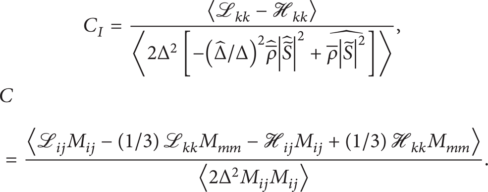
\begin{matrix} C_{I} = \frac{〈 ℒ_{k k} - ℋ_{k k} 〉}{〈 2 Δ^{2} [- {(\hat{Δ} / Δ)}^{2} \hat{\bar{ρ}} {| \hat{\tilde{S}} |}^{2} + \hat{\bar{ρ} {| \tilde{S} |}^{2}}] 〉}, \\ C = \frac{〈 ℒ_{i j} M_{i j} - (1 / 3) ℒ_{k k} M_{m m} - ℋ_{i j} M_{i j} + (1 / 3) ℋ_{k k} M_{m m} 〉}{〈 2 Δ^{2} M_{i j} M_{i j} 〉} . \end{matrix}

(2)

The details of the symbols and modeling can be found in [20]. The subgrid heat flux, given by $Q_{j} = (1 / (γ - 1)) (\bar{p u_{j}} - \bar{p} {\tilde{u}}_{j})$ , is modeled using the eddy diffusivity model as

Q_{j} = - \frac{μ_{t}}{P r_{t}} \frac{\partial \tilde{T}}{\partial x_{j}} = - \frac{C Δ^{2} \bar{ρ} | \tilde{S} |}{P r_{t}} \frac{\partial \tilde{T}}{\partial x_{j}},

(3)

where the SGS Prandtl number Pr_t is chosen to be constant and set equal to 0.5.

A finite difference method is employed to discretize the equations. After the local Steger-Warming flux splitting, the convective terms are discretized with a fifth-order upwind compact difference scheme, which is developed by Fu and Ma [21]. A sixth-order symmetric compact difference scheme developed by Lele [22] is employed for the diffusive terms. The time integration is performed using an explicit third-order three-step Runge-Kutta scheme [23], which satisfies the TVD (Total Variation Diminishing) property. The parallel computation is implemented based on MPI (massage passing interface).

3. Case Description

The computational configuration and coordinate system are displayed in Figure 1. The x-, y-, and z-axes are set along the streamwise, wall-normal, and spanwise directions, respectively, and L_x, L_y, and L_z are the size of the computational domain in the corresponding directions. The entrance of the computational domain corresponded to a location x_in from the leading edge of the flat-plate. The computational domain is x_in ≤ x ≤ L_x + x_in, 0 ≤ y ≤ L_y, and 0 ≤ z ≤ L_z, where the flat-plate is set at y = 0.

Figure 1:

Configuration of a flat-plate flow.

Based on the spatial mode, the initial flow field of the inlet boundary is consisted of two parts: one part is the basic mean flow, and the other part is the disturbances which are introduced to make the transition occur. The inlet flow field can be expressed as

f = \bar{f} + f^{'},

(4)

where the mean flow $\bar{f}$ is the similarity solution of the compressible laminar boundary layer, and f′ consisted of a pair of the most unstable oblique first mode disturbances as

\begin{matrix} f^{'} = A (y) e^{- α_{i} x} \cos (α_{r} x \pm β z - ω t), \\ A (y) = A e^{- b y^{2}} . \end{matrix}

(5)

The values of the coefficients can be found in [11]. The maxima of the streamwise velocity disturbance amplitude are about 2% of the freestream velocity.

Periodic boundary condition is imposed on the spanwise direction, and isothermal nonslip boundary conditions are applied on the flat-plate. In order to effectively implement nonreflecting boundary conditions, the fringe method [24] is adopted for the outlet boundary and the upper boundary. In this method, a buffer region is added to the boundary of the original computational region. In order to decay the reflected wave, the artificial dissipation is added to the governing equation in this region.

The flow and computation parameters are summarized in Table 1, where n_x, n_y, and n_z are, respectively, the number of grid points along the corresponding directions. The reference length is the displacement thickness at the inlet boundary δ_d0, while the reference density, velocity, and temperature are the freestream values. The grid spacing is placed uniformly along the spanwise direction and stretched following a hyperbolic tangent law along the wall-normal direction. The grid is uniform along the streamwise direction where x < 430.85δ_d0, and stretched grid is used as a buffer region downstream.

Table 1:

Flow and computation parameters.

Ma_∞	4.5
Re_δd = ρ_∞V_∞δ_d0/μ_∞	1.0 × 10⁴
δ_d0	Inlet displacement thickness
x _in	90.5 δ_d0
T _∞	61.11 K
T _w	267.66 K (T_w = 4.38 T_∞)
L_x × L_y × L_z	418.88 δ_d0 × 7.57 δ_d0 × 60 δ_d0
n_x × n_y × n_z	983 × 101 × 33

4. Results and Discussion

The average results of flow field are carried out until the computation reached statistical equilibrium. Because the spanwise direction is periodic, the ensemble averages both in time and in spanwise direction are used to obtain the mean values.

4.1. Mean Statistics and Analysis

Figure 2 depicts the skin friction coefficient along the streamwise direction, which is defined as

C_{f} = \frac{τ_{w}}{(1 / 2) ρ_{\infty} V_{\infty}^{2}}, τ_{w} = {\bar{μ \frac{\partial u}{\partial y}} |}_{w} .

(6)

Moreover, the theoretical estimates for the fully turbulent regime given by White [25] are also included in Figure 2. It can be seen that the skin friction increases fast at x ≈ 170δ_d0, which can be defined as the “transition point.” The corresponding transition Reynolds number is about Re_x = 1.7 × 10⁶ or Re_θ = 901. Then, the skin friction rises up quickly between x = 170δ_d0 and x = 240δ_d0 and reaches its maximum at about x = 246δ_d0. When x > 250δ_d0, the skin friction exhibits oscillation and decreases as the boundary layer flow develops into full turbulence. The simulation shows a good agreement with White's results in the fully developed turbulent region. Thus, the present simulation is reliable and valid.

Figure 2:

Distribution of the skin friction coefficient.

The contributions of the velocity fluctuations u′, v′, and w′ to the disturbance energy are denoted by e2u, e2v, and e2w, respectively:

\begin{matrix} e 2 u = \int_{y = 0}^{y = L_{y}} \frac{1}{2} (\bar{u^{' 2}}) d y, \\ e 2 v = \int_{y = 0}^{y = L_{y}} \frac{1}{2} (\bar{v^{' 2}}) d y, \\ e 2 w = \int_{y = 0}^{y = L_{y}} \frac{1}{2} (\bar{w^{' 2}}) d y . \end{matrix}

(7)

Consequently, the disturbance energy e2 is defined as

e 2 = \int_{y = 0}^{y = L_{y}} \frac{1}{2} (\bar{u^{' 2} + v^{' 2} + w^{' 2}}) d y .

(8)

The distributions of e2u, e2v, e2w, and e2 are presented in Figure 3. Clearly, the variation of e2 exhibits a similar trend to the skin friction coefficient. Due to the enlarged growth of various order disturbances in the flow field, the disturbance energy increases during the transition process. The disturbance energy e2 rises up quickly at about x = 150δ_d0 and reaches maximum at about x = 200δ_d0, indicating that it changes before the skin friction coefficient. According to Figure 3, the evolution of e2u shows a similar trend to e2, and the growths of e2v and e2w lag behind e2u. Furthermore, the value of e2u is always greater than e2v and e2w, indicating that the disturbance energy mainly comes from the streamwise velocity fluctuations.

Figure 3:

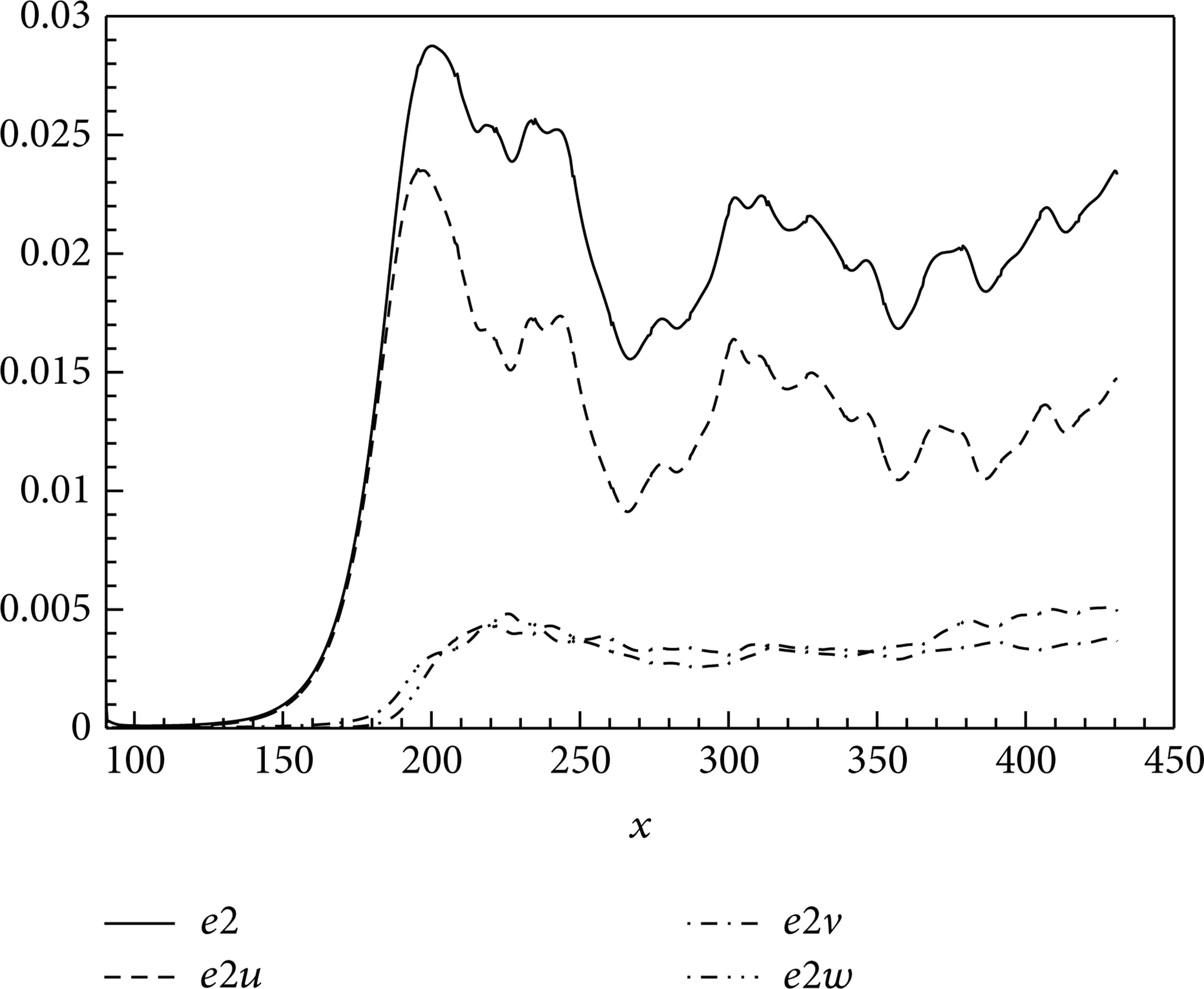
Distribution of the disturbance energy.

Figure 4 shows the profiles of mean flow at different x locations, including the laminar inlet (x = 90.5δ_d0), the transition point (x = 170δ_d0), the middle region of transition zone (x = 210δ_d0), the transition finished point (x = 246δ_d0), and fully developed turbulent region (x = 335, 370, 400, 428δ_d0). It can be seen from Figure 4(a) that the mean streamwise velocity profiles are a typical distribution of laminar flow at x = 90.5δ_d0. The profiles have little change and still maintain laminar flow in region 90.5δ_d0 < x < 170δ_d0. Between x = 170δ_d0 and x = 246δ_d0, the profiles undergo rapid modification and inflexion points appear near the critical layer. The mean velocity profiles with inflexion points lead to instability and accelerate the transition. Between x = 335δ_d0 and x = 428δ_d0, the profiles change slowly and are typical distribution of turbulent flow, indicating that the equilibrium state of fully developed turbulence has been reached. As shown in Figures 4(b) and 4(c), the evolutions of the mean density and temperature along streamwise locations are similar to the mean velocity; namely, the laminar profiles change into turbulent profiles through the transition process.

Figure 4:

Profiles of the mean flow: (a) streamwise velocity, (b) density, and (c) temperature.

The dimensionless mean velocity profiles normalized by the skin friction velocity are given in Figure 5 at the same locations as in Figure 4. It shows that the profiles satisfy the wall law u⁺ = y⁺ in the viscous sublayer 0 ≤ y⁺ ≤ 8 for all locations. Before the completion of transition (x < 250δ_d0), the profiles change greatly and do not satisfy the log law u⁺ = 2.5lny⁺ + 5.5 in the log-law region. For the four locations in fully developed turbulent region, the profiles of log-law region are similar, but they are still different from the log law. Figure 6 shows the mean Van Driest transformative velocity [26] profiles normalized by wall-shear velocity at these four locations. The four are found to well satisfy the log law, especially the slopes of the curves. Compared with incompressible case, the regions of wall law and log-law both enlarge, so the buffer layer is narrower than that of incompressible turbulent flow.

Figure 5:

Profiles of the normalized mean streamwise velocity.

Figure 6:

Profiles of the mean streamwise velocity with Van Driest transformation.

For compressible flow, the displacement thickness δ_d, momentum thickness θ, and shape factor H are defined as

\begin{matrix} δ_{d} = \int_{0}^{δ} (1 - \frac{ρ u}{ρ_{\infty} u_{\infty}}) d y, \\ θ = \int_{0}^{δ} \frac{ρ u}{ρ_{\infty} u_{\infty}} (1 - \frac{u}{u_{\infty}}) d y, \\ H = \frac{δ_{d}}{θ} . \end{matrix}

(9)

The boundary layer thickness δ is defined as the distance from the wall where the mean velocity reaches 99% of the freestream velocity. The thickness of boundary layer and shape factor obtained from the simulation are plotted in Figure 7. The boundary layer thickness has a rapid growth at about x = 190δ_d0 and increases one time at about x = 250δ_d0. The growth rate in transition region is much higher than that in laminar region and then decreases in the fully developed turbulent region. Unlike the boundary layer thickness, the growth rate of the displacement thickness slightly declines after about x = 190δ_d0 and then rises in the fully developed turbulent region (x > 250δ_d0). The momentum thickness increases fast at about x = 170δ_d0, which is prior to the boundary layer thickness. The momentum thickness increases by about one time at about x = 250δ_d0, and then the growth rate decreases. The values of the shape factor in laminar flow region remain a constant value of about 15.8 and drop significantly at x ≈ 170δ_d0. When x > 250δ_d0, the shape factor changes in a small range and the average value is around 9. Maeder et al. [4] obtained the shape factor of 8.91 based on temporal DNS at the same Mach number and Reynolds number, indicating that the present simulation is reliable. It also can be seen from Figure 7 that the growth rate in turbulent region is larger than that in laminar region for all three thicknesses of boundary layer.

Figure 7:

Distributions of various thicknesses of boundary layer and shape factor: (a) boundary layer thickness; (b) displacement thickness; (c) momentum thickness; and (d) shape factor.

4.2. Statistics and Analysis about Turbulent Fluctuations

The turbulent Mach number M_t is defined as

M_{t} = \frac{\sqrt{\bar{u^{' 2} + v^{' 2} + w^{' 2}}}}{\bar{a}},

(10)

where $\bar{a}$ is the local average speed of sound. The turbulent Mach number is a physical quantity to describe the intrinsic compressibility effects. According to Morkovin's hypothesis [27], the influences of compressibility effects can be ignored when the turbulent Mach number is not greater than 0.3. Figure 8 shows the profiles of the turbulent Mach number at different x locations. Due to the addition of disturbances, the near-wall value of the turbulent Mach number is not zero at the inlet boundary x = 90.5δ_d0. With the development of the disturbances, it appears to be a certain distribution in the near-wall region at the transition point x = 170δ_d0. The overall distribution and the peak value of the turbulent Mach number are larger at x = 210δ_d0 and x = 246δ_d0, indicating that the turbulent fluctuations are comparatively stronger in the transition region. The profiles of the four locations in fully developed turbulent region are similar, and all reach the maximum values around y⁺ = 13. The peak value of the turbulent Mach number is 0.45 at x = 428δ_d0, and the Reynolds number based on the momentum thickness is Re_θ = 3306. Comparatively, Maeder et al. [4] obtained a peak value of 0.41 at Re_θ = 3305. Moreover, the distributions of the turbulent Mach number in fully developed turbulent region are greater than 0.3 for 6 < y⁺ < 50, indicating that the compressible effects are noticeable.

Figure 8:

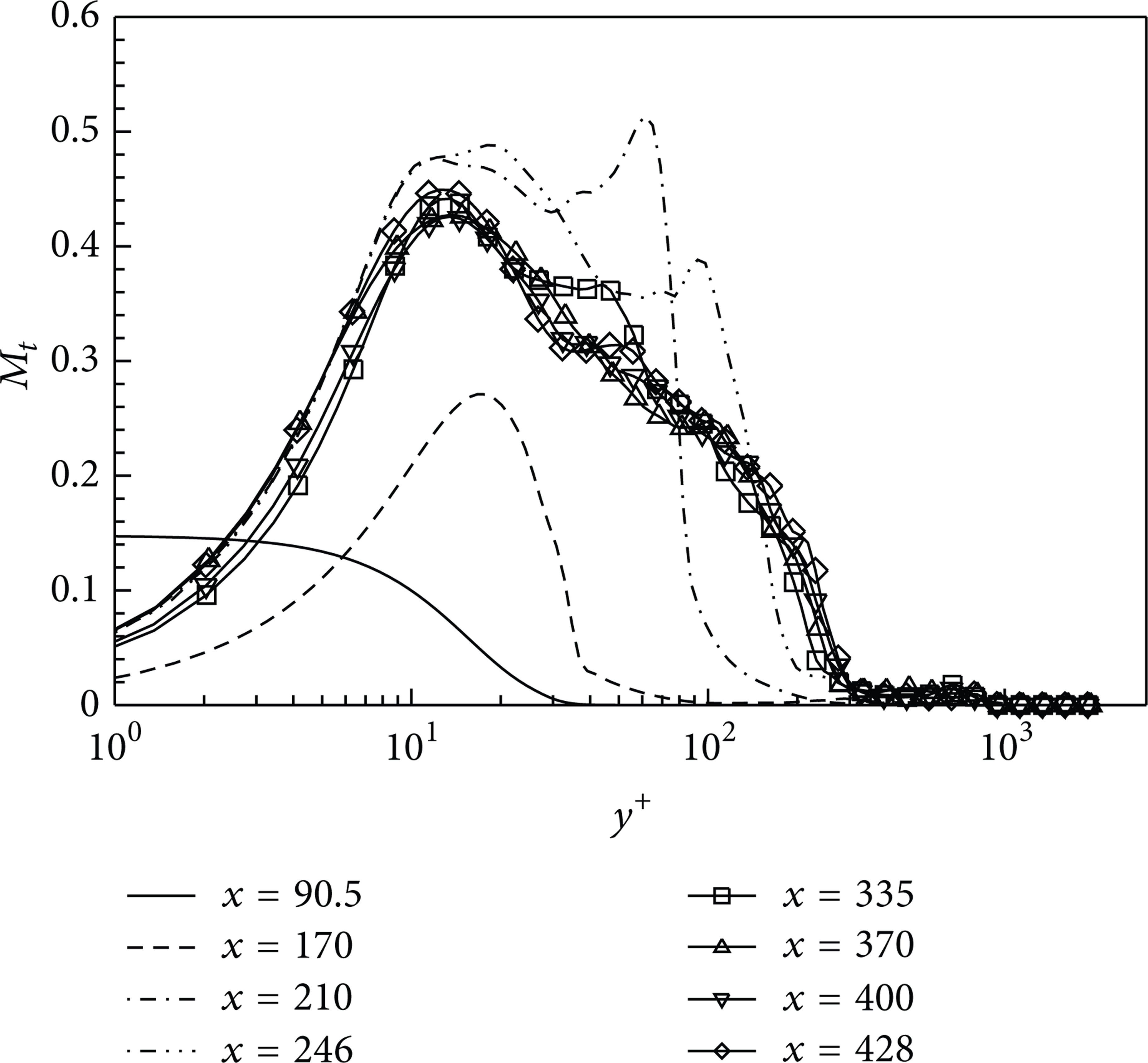
Profiles of the turbulent Mach number.

The rms density, temperature, and pressure fluctuations normalized by the mean profiles are presented in Figure 9.

Figure 9:

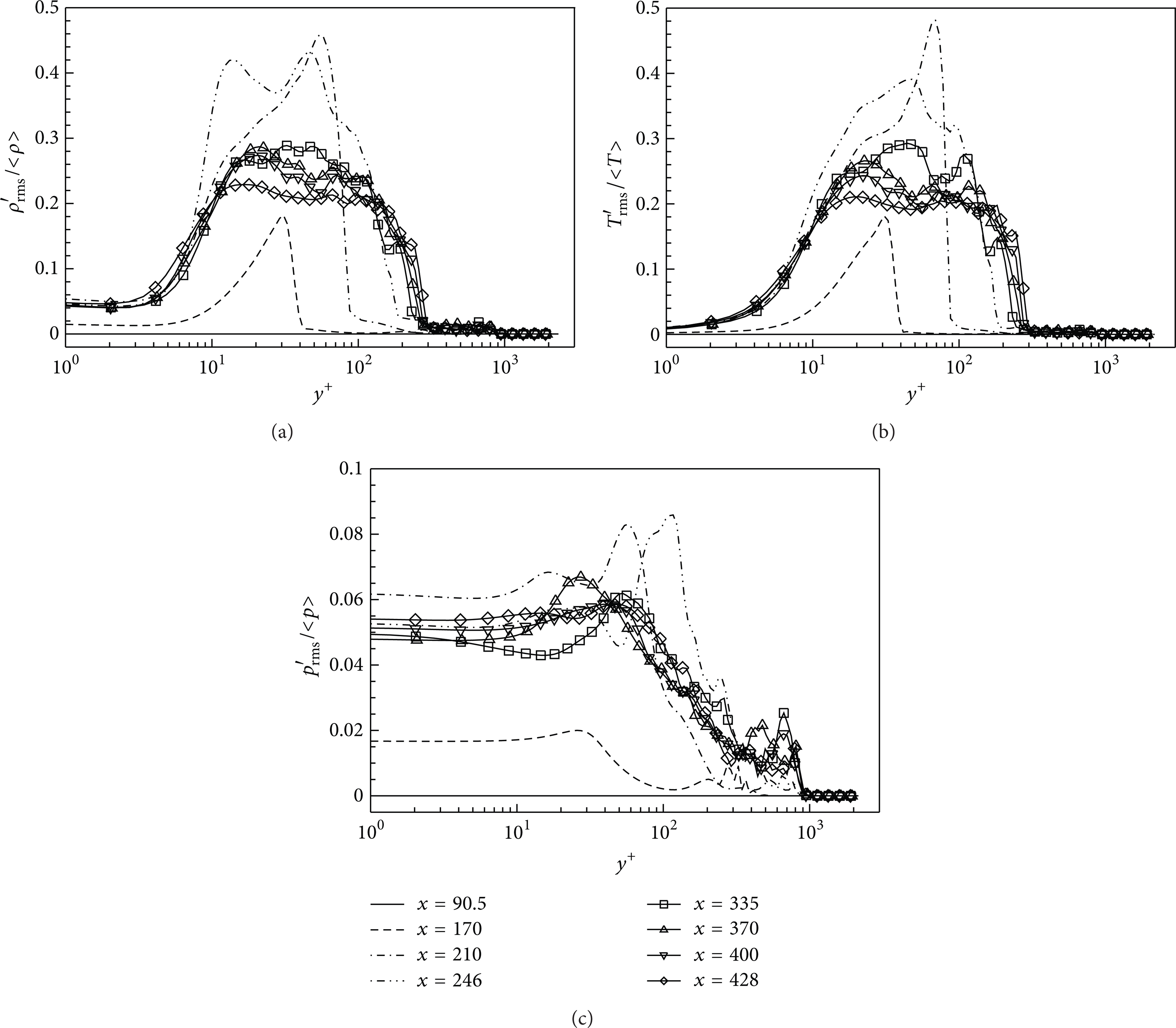
Profiles of the rms fluctuation quantities: (a) density, (b) temperature, and (c) pressure.

As shown in Figure 9(a), the distributions of the rms density fluctuations increase gradually along the downstream and reach larger value in the transition process. The profiles of the fully developed turbulent region have similarity, and the maximum value is close to 0.3. It can also be found that the rms density fluctuations are greater than 0.1 in a wide range of the boundary layer (8 < y⁺ < 200), indicating that the density fluctuations cannot be ignored. According to Figure 9(b), the distributions of the rms temperature fluctuations show a similar trend to those of the density, and the maximum value in the fully developed turbulent region is close to 0.3. Figure 9(c) shows that the distributions of the rms pressure fluctuations remain constant in the viscous sublayer and then decrease gradually. The profiles of the fully developed turbulent region also have similarity, and the overall distributions are below 0.06.

Figure 10 shows the profiles of the normalized Reynolds stress for the four x locations in fully developed turbulent region. Clearly, the distributions of the Reynolds stress show similarity, and the values are small in the viscous sublayer and close to zero when y⁺ > 300. It can be seen that the streamwise Reynolds normal stress is much larger than others, and its peak value reaches 11, which is different from the result 7 of Kim et al. [28] for incompressible turbulent flow. However, the position of the peak value has little difference; for the present simulation it is y⁺ ≈ 12, and for Kim et al. [28] it is y⁺ ≈ 15. According to Figures 10(b)–10(d), the peak values of the wall-normal and spanwise Reynolds normal stress and the Reynolds shear stress in xy plane are 1.3, 2, and 1, respectively, while the corresponding results of Kim et al. [28] are 0.7, 1.2, and 0.7. Therefore, the Reynolds stress for compressible turbulence becomes larger compared with the incompressible turbulence.

Figure 10:

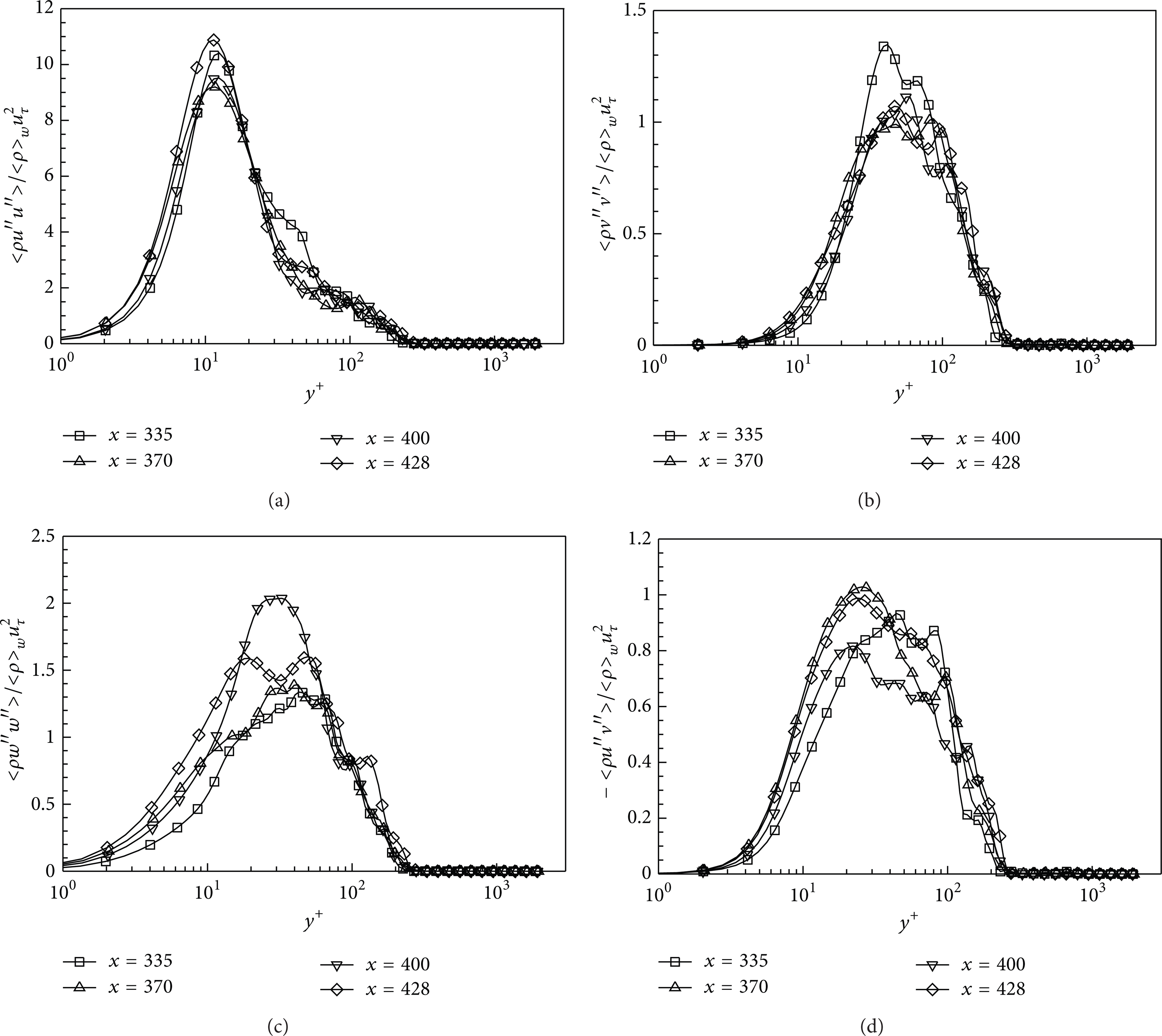
Profiles of the Reynolds stress: (a) streamwise Reynolds normal stress, (b) wall-normal Reynolds normal stress, (c) spanwise Reynolds normal stress, and (d) Reynolds shear stress in xy plane.

4.3. Large-Scale Coherent Structures

The dominant feature of the transitional flow is the existence of complex vortex structures, including Λ vortices, hairpin vortices, and ring-like vortices. Figure 11 shows the instantaneous isosurface of Q = 0.02, where Q is the second invariant of the velocity gradient tensor. As shown in Figure 11(a), the Λ vortices are visible between x = 170δ_d0 and x = 180δ_d0, but it is not obvious. A series of open-tip Λ vortices are observed between x = 180δ_d0 and x = 210δ_d0, and these Λ vortices are staggered in the streamwise direction, that is, the typical characteristics of the H-type subharmonic transition. Starting from x = 210δ_d0, the tips of the Λ vortices are lifted downstream by the motion induced by the tails of other Λ vortices. Because the streamwise velocity increases gradually away from the wall, the Λ vortices have been stretched and undergone deformation by the shear effect, forming hairpin-like vortices which have close tips and open tails. Subsequently, the tips of the hairpin vortices continue to be lifted and the two legs are constantly close to each other, forming ring-like vortices. When x > 250δ_d0, the heads of the ring-like vortices are broken, leading to the generation of some small-scale structures. This indicates that the transition process tends to finish. It can be seen from Figure 11(b) that there are no large-scale coherent structures in the fully developed turbulent region, and the random distribution of the small scale vortices is apparent.

Figure 11:

Instantaneous isosurface of Q = 0.02. (a) Transition region; (b) fully developed turbulent region (data duplicated periodically in the spanwise direction).

5. Conclusions and Remarks

Large eddy simulation of a spatially developing supersonic flat-plate boundary layer from the laminar through transition process to fully developed turbulence with Ma_∞ = 4.5 has been carried out. Some conclusions and remarks can be stated as follows.

Through the development of the initial perturbations, the mean velocity, density, and temperature profiles vary rapidly, resulting in the rapid growth of the skin friction. The streamwise location for the rapid change of the momentum thickness is the same as the skin friction, whereas that of the boundary layer thickness and displacement thickness is a little downstream. Although the starting positions for rapid change of these quantities are not consistent, but the ending positions are basically the same, namely, where the transition process has finished.

The profiles of turbulent Mach number, rms fluctuation quantities, and Reynolds stresses along the wall-normal direction at different streamwise locations exhibit self-similarity in fully developed turbulence. The values of these relevant quantities in transition process will appear larger than that in fully developed turbulent region.

The values of the turbulent Mach number and rms density fluctuations are both greater than the corresponding critical values of Morkovin's hypothesis in a wide range of the boundary layer, indicating that the compressibility effects cannot be ignored under the present conditions.

Through the instantaneous isosurface of the second invariant of the velocity gradient tensor, the onset and development of Λ vortices, hairpin vortices, ring-like vortices, and the broken of ring-like vortices are depicted.

Conflict of Interests

The authors declare that they have no conflict of interests regarding the publication of this paper.

References

Dinavahi

S. P. G.

Pruett

C. D.

, and Zang

T. A.

, “Direct numerical simulation and data analysis of a Mach 4.5 transitional boundary-layer flow,” Physics of Fluids, vol. 6, no. 3, pp. 1323–1330, 1994.

Adams

N. A.

and Kleiser

, “Subharmonic transition to turbulence in a flat-plate boundary layer at Mach number 4.5,” Journal of Fluid Mechanics, vol. 317, pp. 301–335, 1996.

Guarini

S. E.

Moser

R. D.

Shariff

, and Wray

, “Direct numerical simulation of a supersonic turbulent boundary layer at Mach 2.5,” Journal of Fluid Mechanics, vol. 414, pp. 1–33, 2000.

Maeder

Adams

N. A.

, and Kleiser

, “Direct simulation of turbulent supersonic boundary layers by an extended temporal approach,” Journal of Fluid Mechanics, vol. 429, pp. 187–216, 2001.

Pirozzoli

Grasso

, and Gatski

T. B.

, “Direct numerical simulation and analysis of a spatially evolving supersonic turbulent boundary layer at M = 2.25,” Physics of Fluids, vol. 16, no. 3, pp. 530–545, 2004.

Huang

Cao

, and Zhou

, “Mechanism of breakdown in laminar-turbulent transition of a supersonic boundary layer on a flat plate-temporal mode,” Science in China Series G, vol. 48, no. 5, pp. 614–625, 2005.

Cao

Huang

Z.-F.

, and Zhou

, “Study of mechanism of breakdown in laminar-turbulent transition of supersonic boundary layer on flat plate,” Applied Mathematics and Mechanics, vol. 27, no. 4, pp. 425–434, 2006.

X.-L.

D.-X.

, and Ma

Y.-W.

, “Direct numerical simulation of a spatially evolving supersonic turbulent boundary layer at Ma = 6,” Chinese Physics Letters, vol. 23, no. 6, pp. 1519–1522, 2006.

Liang

and Li

X. L.

, “DNS of a spatially evolving hypersonic turbulent boundary layer at Mach 8,” Science China Physics, Mechanics and Astronomy, vol. 56, no. 7, pp. 1408–1418, 2013.

10.

El-Hady

N. M.

and Zang

T. A.

, “Large-eddy simulation of nonlinear evolution and breakdown to turbulence in highspeed boundary layers,” Theoretical and Computational Fluid Dynamics, vol. 7, no. 3, pp. 217–240, 1995.

11.

Shan

Jiang

Zhao

, and Liu

, “Large eddy simulation of flow transition in a supersonic flat-plate boundary layer,” in Proceedings of the 37th Aerospace Sciences Meeting and Exhibit, AIAA paper 99-0425, Reno, Nev, USA, January 1999.

12.

Stolz

Schlatter

, and Kleiser

, “Large-eddy simulations of subharmonic transition in a supersonic boundary layer,” AIAA Journal, vol. 45, no. 5, pp. 1019–1027, 2007.

13.

Pan

H.-L.

H.-D.

, and Wang

, “Large eddy simulation of transition coherent structures in a supersonic boundary layer,” Journal of Astronautics, vol. 27, no. 3, pp. 498–502, 2006 (Chinese).

14.

Pan

H.-L.

H.-D.

, and Wang

, “Large eddy simulation of transition in a hypersonic blunt-wedge boundary layer,” Acta Aeronautica et Astronautica Sinica, vol. 28, no. 2, pp. 269–274, 2007 (Chinese).

15.

Mary

and Sagaut

, “Large eddy simulation of flow around an airfoil near stall,” AIAA Journal, vol. 40, no. 6, pp. 1139–1145, 2002.

16.

Garnier

Sagaut

, and Deville

, “Large eddy simulation of shock/boundary-layer interaction,” AIAA Journal, vol. 40, no. 10, pp. 1935–1944, 2002.

17.

Teramoto

, “Large-eddy simulation of transitional boundary layer with impinging shock wave,” AIAA Journal, vol. 43, no. 11, pp. 2354–2363, 2005.

18.

Vreman

Geurts

, and Kuerten

, “Subgrid-modelling in LES of compressible flow,” Applied Scientific Research, vol. 54, no. 3, pp. 191–203, 1995.

19.

Wang

S. Z.

Gao

Z. X.

, and Lee

C. H.

, “Numerical investigation of compressibility effects in turbulent channel flows using large eddy simulation,” Science China Physics, Mechanics and Astronomy, vol. 55, no. 2, pp. 305–315, 2012.

20.

Zang

Y. Z. Yan

Street

R. L.

, and Koseff

J. R.

, “A dynamic mixed subgrid-scale model and its application to turbulent recirculating flows,” Physics of Fluids A, vol. 5, no. 12, pp. 3186–3196, 1993.

21.

D. X.

and Ma

Y. W.

, “High order accurate schemes and numerical simulation of multi-scale structures in complex flow fields,” Acta Aerodynamica Sinica, vol. 16, no. 1, pp. 24–35, 1998 (Chinese).

22.

Lele

S. K.

, “Compact finite difference schemes with spectral-like resolution,” Journal of Computational Physics, vol. 103, no. 1, pp. 16–42, 1992.

23.

Gottlieb

and Shu

C.-W.

, “Total variation diminishing Runge-Kutta schemes,” Mathematics of Computation, vol. 67, no. 221, pp. 73–85, 1998.

24.

Kloker

Konzelmann

, and Fasel

, “Outflow boundary conditions for spatial Navier-Stokes simulations of transition boundary layers,” AIAA Journal, vol. 31, no. 4, pp. 620–628, 1993.

25.

White

F. M.

, Viscous Fluid Flow, McGraw-Hill, New York, NY, USA, 2nd edition, 1991.

26.

Coleman

G. N.

Kim

, and Moser

R. D.

, “Numerical study of turbulent supersonic isothermal-wall channel flow,” Journal of Fluid Mechanics, vol. 305, pp. 159–183, 1995.

27.

Morkovin

M. V.

, “Effects of compressibility on turbulent flows,” in Mechanique de la Turbulence, Gordon & Breach, New York, NY, USA, 1964.

28.

Kim

Moin