Smooth and Accurate Trajectory Planning for Industrial Robots

Abstract

This paper proposes a smooth and accurate trajectory planning for industrial robots using geodesics. The workspace of a robot is split into positional and orientational parts. A Riemannian metric is given on each space such that the desired motion is a geodesic for the given metric. By regarding joint variables as local coordinates of the position space and the orientation space, Cartesian trajectories are represented by joint trajectories. A smooth and accurate motion of the robot end-effector and smooth joint trajectories corresponding to the motion can be obtained by calculating geodesics on the position space and the orientation space. To demonstrate the effectiveness of the proposed method, simulation experiments are conducted using the PUMA 560 robot.

1. Introduction

Industrial robots are used in many different industrial applications, like handling, machining, arc welding, and painting. In some cases, such as machining, arc welding, and painting, it is important that a robot end-effector moves accurately and in a smooth continuous manner along a specified trajectory. For example, in a machining process a robot end-effector may be required to move a tool for cutting a three-dimensional surface smoothly.

Olabi et al. presented a method of trajectory planning adapted for continuous machining by robots [1]. In this method, a smooth motion law was generated by means of a parametric speed interpolator. Ning et al. proposed a method for trajectory generation based on dynamic movement primitives [2]. They generated smooth trajectories which satisfied position and velocity boundary conditions at start and end points with high precision. Boryga and Graboś presented a planning mode of manipulator motion trajectory with higher-degree polynomials [3]. Gasparetto and Zanotto developed a method for smooth trajectory planning of robot manipulators [4]. They worked out an objective function containing a term proportional to the integral of the squared jerk (to ensure that the trajectory is smooth) and the second term, proportional to the total execution time. Liu et al. presented a smooth trajectory planning method which was designed as a combination of the planning with multidegree splines in the Cartesian space and multidegree B-splines in the joint space [5]. Yang and Sukkarieh proposed an analytical continuous-curvature path-smoothing algorithm which was based upon parametric cubic $\acute{\text{B}}$ ezier curves [6].

However, the trajectory planning methods are often using interpolating functions, and the interpolating is performed either in the joint space or the Cartesian space. In joint space schemes, in order to obtain accurate trajectories, planning can be done by interpolating a sequence of via points, but the motion actually performed by the robot end-effector between these via points is not easily foreseeable. On the other hand, because of the nonlinearity of the inverse kinematics, a smooth trajectory in the Cartesian space may cause a nonsmooth joint motion when the interpolated data in the Cartesian space are mapped into the joint space and consequently a nonsmooth and inaccurate motion in the Cartesian space.

Since the end of the 20th century, geodesics have been introduced into robotics for path planning. Geodesic, which is the necessary condition of the shortest length between two points on a Riemannian manifold, is intrinsic and has no relation with coordinates [7]. The joints of a robot are regarded as linearly dependent in the geodesic method [8].

Rodnay and Rimon visualized the dynamic properties of a 2 DOFs (degrees of freedom) robot in the three-dimensional Euclidean space [9]. They introduced geodesics on the dynamic surface to represent trajectories when the robot system made free motions. Using the notions of the Riemannian metric and the covariant derivative, Žefran et al. focused on the generation of smooth three-dimensional rigid body motions which were Cartesian space schemes in their paper [7]. Tchoń and Duleba addressed on inverting singular kinematics [10]. An advantage of their method was that the workspace locations generated by the method lay on a straight line. However, the method was based upon the so-called generalized Newton algorithm and the straight line was planned point by point using the inverse kinematics. Selig and Ovseevitch sought to combine the control and the trajectory planning and manipulate robots along helical trajectories [11]. They applied the Lie algebra and the Lie group which often made the planning abstruse, abstract, and not easy to put into practice. Zhang et al. regarded the arc length and the kinetic energy as Riemannian metrics to achieve the shortest path and the invariant kinetic energy trajectories, respectively [8, 12]. But when they used the arc length as the Riemannian metric, they actually could not plan trajectories of robots with more than 3 DOFs and the orientation problem had not been tackled.

In order to overcome the above-mentioned problems, this paper proposes a smooth and accurate trajectory planning using geodesics. The workspace of a robot is split into positional and orientational parts. Riemannian metrics are then given on the two spaces such that the desired motions are geodesics for the given metrics. It allows them to generate trajectories that include the position and the orientation. By regarding joint variables as local coordinates of the position space and the orientation space and calculating geodesics on them, Cartesian trajectories are represented by joint trajectories. Because of the geometric characteristics of geodesics, Cartesian trajectories and corresponding joint trajectories are both smooth and accurate.

As mentioned above, the distance length and kinematic energy were regarded as Riemannian metrics, respectively, in previous studies. The proposed method splits the workspace into positional and orientational parts and uses two Riemannian metrics: the distance metric and the orientation metric. The shortest paths of a robot with more than 3 DOFs and orientation trajectories can be obtained using geodesics, while these are not considered adequately in the previous works. Traditional methods often require a constant solution to the inverse kinematics. The interpolating is performed either in the joint space or the Cartesian space, and the joint scheme and the Cartesian scheme are often separate. The constant solution to the inverse kinematics and the separation of joint schemes and Cartesian schemes may cause the planned trajectories nonsmooth or inaccurate. The immediate output of the geodesic method which selects joint variables as local coordinates is joint trajectories, and the Cartesian trajectory obtained by the forward kinematics is exactly the planning geodesic path. The geodesic method requires only the inverse kinematic solutions of endpoints.

2. Background of Geodesic

To begin with, we provide a brief background on geodesics.

2.1. Manifold and Local Coordinate

A manifold M ⁿ is a Hausdorff topological space for which each point p has a neighborhood U⊂M ⁿ homeomorphic to an open subset of the Euclidean space R ⁿ [13]. If φ:U → φ(U)⊂R ⁿ (φ(U) is open) is the homeomorphism and denotes x ⁱ (p)≐(φ(p)) ⁱ , we say that (U;x ⁱ ) is a local coordinate system of M and x ⁱ (i = i,…, n) are local coordinates.

2.2. Riemannian Manifold

Let (M ⁿ , g) be a Riemannian manifold; that is, M ⁿ is an n-dimensional differentiable manifold and g is a Riemannian metric. A Riemannian metric g is a symmetric, positive definite quadratic form. Let {θ _i }_{i = 1} ⁿ be local coordinates in a neighborhood U of a point of M. The metric may be written in local coordinates as

$g={\displaystyle \sum }_{i,j=\mathrm{1}}^n‍g_{ij}d{\theta }_{i}d{\theta }_j,$

(1)

where g _ij ≐g(∂/∂θ _i , ∂/∂θ _j ) and d, ∂ refer to the differential and the partial differential, respectively [14, 15].

2.3. Geodesic

Let γ:I → M be a smooth curve. In a local coordinate system, it can be written as

${\theta }_i={\theta }_i\left(t\right),\hspace{1em}t\in I,\hspace{0.17em}\hspace{0.17em}i=\mathrm{1,2},\dots ,n.$

(2)

We say that γ is a geodesic if and only if it satisfies the geodesic equations

$\frac{d^{\mathrm{2}}{\theta }_i}{d{t}^{\mathrm{2}}}+{\displaystyle \sum }_{k,j=\mathrm{1}}^n‍{\Gamma }_{kj}^i\frac{d{\theta }_k}{dt}\frac{d{\theta }_j}{dt}=\mathrm{0},\hspace{1em}i=\mathrm{1,2},\dots ,n.$

(3)

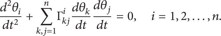
The Christoffel symbols Γ _kj ⁱ are given in terms of the Riemannian metric by

${\Gamma }_{kj}^i=\frac{\mathrm{1}}{\mathrm{2}}{\displaystyle \sum }_{m=\mathrm{1}}^n‍g^{mi}\left(\frac{\partial g_{km}}{\partial {\theta }_j}+\frac{\partial g_{jm}}{\partial {\theta }_k}-\frac{\partial g_{kj}}{\partial {\theta }_m}\right),$

(4)

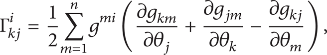
where g ^mi is the element of the inverse Riemannian metric coefficient matrix [16].

3. Smooth and Accurate Trajectory Planning Using Geodesics

Once the link frames have been attached and the corresponding link parameters have been found, the kinematical equations are straightforwardly determined. Assume that the T matrix of a robot end-effector is

$T=\left(\begin{array}{cc}R& p\\ \mathrm{0}& \mathrm{1}\end{array}\right)=\left(\begin{array}{cccc}{n}_x& o_x& a_x& p_x\\ n_y& o_y& a_y& p_y\\ n_z& o_z& a_z& p_z\\ \mathrm{0}& \mathrm{0}& \mathrm{0}& \mathrm{1}\end{array}\right),$

(5)

where n = o × a, o·o = 1, a·a = 1, o·a = 0 [17].

3.1. Local Coordinates and the Selection Mode

To combine joint space schemes and Cartesian space schemes, a relationship between the joint space and the Cartesian space should be established. A nature idea is to select the set of all joint variables as a coordinate system of the Cartesian space. The forward kinematics gives a description from the joint space to the Cartesian space. Specifically, given a set of joint angles, the position and the orientation of the tool frame relative to the base frame are definite. Conversely, given a coordinate which represents the position and the orientation of the tool frame relative to the base frame, the joint coordinates may be indefinite, because the inverse solution is not always unique or even existent. There is often no one-to-one mapping between the Cartesian space and the joint space. For this reason, the set of all joint variables cannot be regarded as a coordinate system of the Cartesian space.

Although joint variables cannot be regarded as coordinates of the Cartesian space, they can be selected as local coordinates. The workspace of a robot is split into its positional and orientational parts. Some joint variables are selected as local coordinates of the position space, and others are regarded as local coordinates of the orientation space.

3.2. Trajectory Planning for Linear Motions Using Geodesics

A line is the only geodesic in the Euclidean space with the distance metric. The position space can be viewed as a Euclidean space and the distance metric of the position space is

$g_d={\left(dp\right)}^{\mathrm{2}},$

(6)

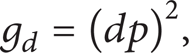
where dp is the derivative of the position vector p = (p _x , p _y , p _z ). A manipulator trajectory planning approach in [8] was proposed by using this metric. But the position is only related to no more than three variables. For a robot whose DOFs are more than three, the trajectory planning approach using the metric g _d only makes part of joints move while movements of others are unknown or still.

Normally, the orientation of the tool frame along a path is defined by the task and cannot be freely selected. On the orientation space, define the Riemannian metric g _o as follows:

$g_o={\left(dn\right)}^{\mathrm{2}}+{\left(do\right)}^{\mathrm{2}}+{\left(da\right)}^{\mathrm{2}},$

(7)

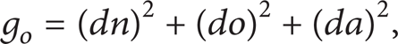
where dn, do, and da are the derivatives of the orientation vectors n = (n _x , n _y , n _z ), o = (o _x , o _y , o _z ), and a = (a _x , a _y , a _z ), respectively.

Both the dimensions of the position space and the orientation space are no more than three. Trajectories of a robot with no more than six DOFs can be planned. If a robot has more than six DOFs, an extra metric which focuses on task constraints or dynamic optimizations should be constructed to get redundant joint trajectories. The flow graph of the trajectory planning using geodesics is shown in Figure 1.

Figure 1:

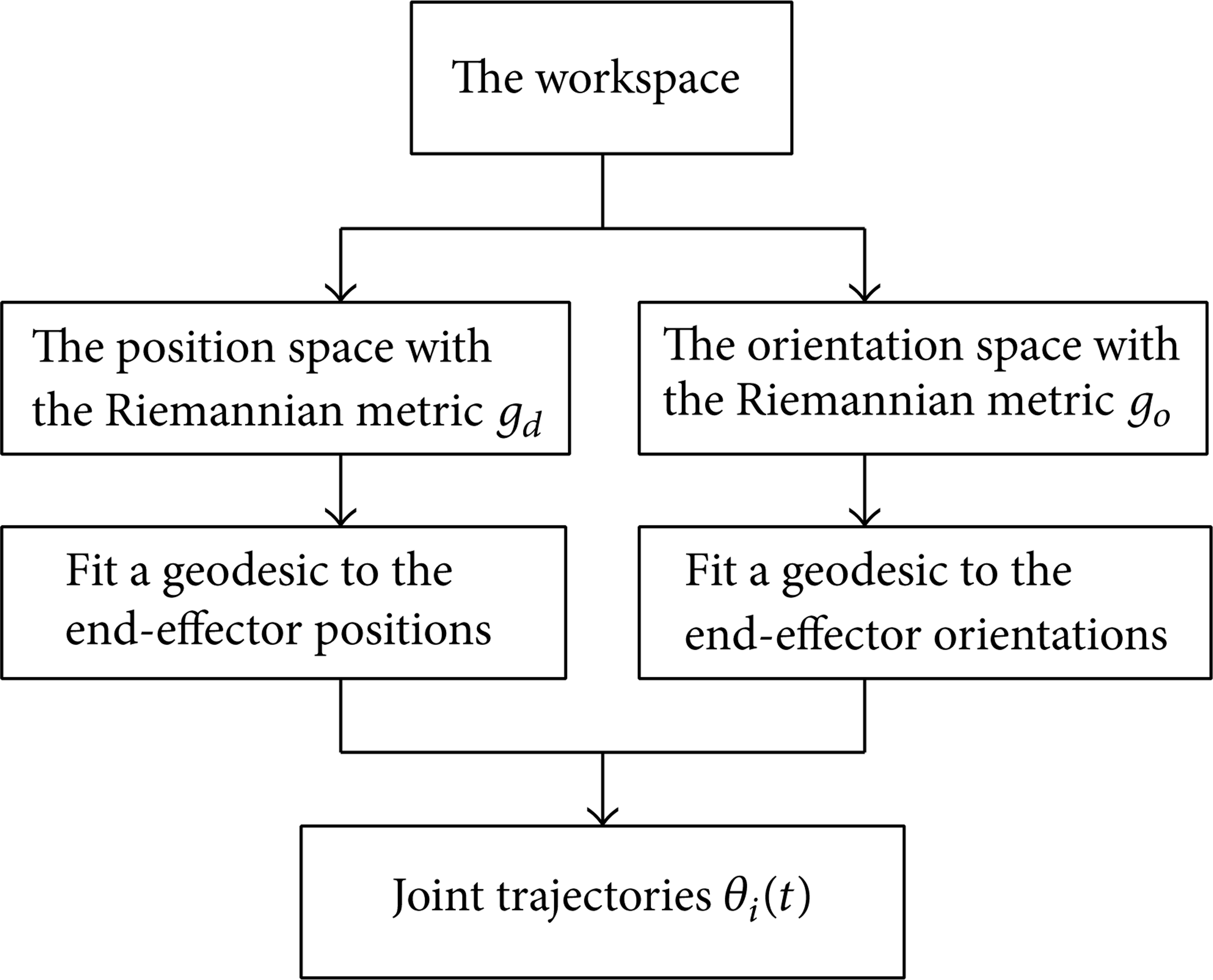
A flowchart of the trajectory planning using geodesics.

3.3. The Evaluation Criterion of the Riemannian Metric Selection

The key point of the geodesic method is finding a suitable metric given the desired trajectory. First of all, a metric should be a symmetric, positive definite quadratic form. Secondly, a metric should be a measure of distance, energy, or other aspects that depend on the desired motions. Geodesic is the necessary condition of the shortest length which is measured by the metric. For example, g _d is a distance metric which measures the distance and a geodesic corresponding to g _d is the shortest path. Finally, the relationship between the amount of a robot DOFs and the dimension of the Riemannian manifold corresponding to the selected metric should be focused on. Often, little attention is devoted to the Riemannian manifold. When the amount of robot DOFs is more than the dimension of the Riemannian manifold, something goes wrong. To avoid a constant solution to the inverse kinematics, a geodesic is desired to be represented by joint trajectories, which can be implemented by choosing the joint variables as local coordinates. The amount of the DOFs should be no more than the dimension of the Riemannian manifold. If not, two or more Riemannian manifolds and their metrics should be constructed, which provides the possibility of multiobjective optimization.

3.4. Computational Considerations

Generally, when a Riemannian metric is given, put it in the form of the coefficient matrix

$g=\left(\begin{array}{cccc}d{\theta }_{\mathrm{1}}& d{\theta }_{\mathrm{2}}& \cdots & d{\theta }_n\end{array}\right)G\left(\begin{array}{c}d{\theta }_{\mathrm{1}}\\ d{\theta }_{\mathrm{2}}\\ ⋮\\ d{\theta }_n\end{array}\right),$

(8)

where G = (g _ij )_{n × n} is the coefficient matrix of the Riemannian metric and θ _i (i = 1,…, n) are joint positions which can be linear or angular. With the coefficient matrix G, we can calculate the Christoffel symbols Γ _kj ⁱ by (4). Then the geodesic equations are obtained with the form as (3).

With the Riemannian metrics g _d and g _o , two sets of geodesic equations with the form as (3) are obtained. These equations and boundary conditions constitute simultaneous differential equations. The solutions of the simultaneous differential equations give the joint trajectories which represent the desired linear motion of the robot end-effector.

In many practical systems, the calculating time is a consideration. The computational efficiency is mainly related to the solution to geodesic equations which are second-order nonlinear ordinary differential equations. The second-order differential equations can be converted to a first-order system. The differential equations are approximated by finite difference equations which are algebraic equations. Unlike initial value problems, a boundary value problem probably does not have a unique solution. Because of this, an initial guess for the desired solution should be provided [18].

For example, the function bvp4c in MATLAB solves two-point boundary value problems for ordinary differential equations [19]. bvp4c produces a solution that is continuous and has a continuous first derivative [20]. The solution is fourth-order accurate uniformly. Six-order accuracy can be got by a sixth-order solver bvp6c which not only supplies greater accuracy, but also performs more efficiently [21]. One also can write a C++ program to get the solution of the geodesic equations with high calculation speed and high accuracy.

3.5. Trajectory Planning for the PUMA 560 Robot Using Geodesics

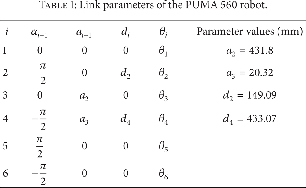
To illustrate the whole trajectory planning procedure using geodesics, the PUMA 560 robot is taken for example. The PUMA 560 robot and its link parameters are shown in Figure 2 and Table 1. The T matrix of the robot end-effector is with the form as (5), where

$\begin{array}{c}{n}_x=c_{\mathrm{1}}\left[c_{\mathrm{23}}\left(c_{\mathrm{4}}{c}_{\mathrm{5}}{c}_{\mathrm{6}}-s_{\mathrm{4}}{s}_{\mathrm{6}}\right)-s_{\mathrm{23}}{s}_{\mathrm{5}}{c}_{\mathrm{6}}\right]+s_{\mathrm{1}}\left(s_{\mathrm{4}}{c}_{\mathrm{5}}{c}_{\mathrm{6}}+c_{\mathrm{4}}{s}_{\mathrm{6}}\right),\\ n_y=s_{\mathrm{1}}\left[c_{\mathrm{23}}\left(c_{\mathrm{4}}{c}_{\mathrm{5}}{c}_{\mathrm{6}}-s_{\mathrm{4}}{s}_{\mathrm{6}}\right)-s_{\mathrm{23}}{s}_{\mathrm{5}}{c}_{\mathrm{6}}\right]-c_{\mathrm{1}}\left(s_{\mathrm{4}}{c}_{\mathrm{5}}{c}_{\mathrm{6}}+c_{\mathrm{4}}{s}_{\mathrm{6}}\right),\\ n_z=-s_{\mathrm{23}}\left(c_{\mathrm{4}}{c}_{\mathrm{5}}{c}_{\mathrm{6}}-s_{\mathrm{4}}{s}_{\mathrm{6}}\right)-c_{\mathrm{23}}{s}_{\mathrm{5}}{c}_{\mathrm{6}},\\ o_x=c_{\mathrm{1}}\left[c_{\mathrm{23}}\left(-c_{\mathrm{4}}{c}_{\mathrm{5}}{s}_{\mathrm{6}}-s_{\mathrm{4}}{c}_{\mathrm{6}}\right)+s_{\mathrm{23}}{s}_{\mathrm{5}}{s}_{\mathrm{6}}\right]+s_{\mathrm{1}}\left(-s_{\mathrm{4}}{c}_{\mathrm{5}}{s}_{\mathrm{6}}+c_{\mathrm{4}}{c}_{\mathrm{6}}\right),\\ o_y=s_{\mathrm{1}}\left[c_{\mathrm{23}}\left(-c_{\mathrm{4}}{c}_{\mathrm{5}}{s}_{\mathrm{6}}-s_{\mathrm{4}}{c}_{\mathrm{6}}\right)+s_{\mathrm{23}}{s}_{\mathrm{5}}{s}_{\mathrm{6}}\right]-c_{\mathrm{1}}\left(-s_{\mathrm{4}}{c}_{\mathrm{5}}{s}_{\mathrm{6}}+c_{\mathrm{4}}{c}_{\mathrm{6}}\right),\\ o_z=-s_{\mathrm{23}}\left(-c_{\mathrm{4}}{c}_{\mathrm{5}}{s}_{\mathrm{6}}-s_{\mathrm{4}}{c}_{\mathrm{6}}\right)+c_{\mathrm{23}}{s}_{\mathrm{5}}{s}_{\mathrm{6}},\\ a_x=-c_{\mathrm{1}}\left(c_{\mathrm{23}}{c}_{\mathrm{4}}{s}_{\mathrm{5}}+s_{\mathrm{23}}{c}_{\mathrm{5}}\right)-s_{\mathrm{1}}{s}_{\mathrm{4}}{s}_{\mathrm{5}},\\ a_y=-s_{\mathrm{1}}\left(c_{\mathrm{23}}{c}_{\mathrm{4}}{s}_{\mathrm{5}}+s_{\mathrm{23}}{c}_{\mathrm{5}}\right)+c_{\mathrm{1}}{s}_{\mathrm{4}}{s}_{\mathrm{5}},\\ a_z=s_{\mathrm{23}}{c}_{\mathrm{4}}{s}_{\mathrm{5}}-c_{\mathrm{23}}{c}_{\mathrm{5}},\\ p_x=c_{\mathrm{1}}\left[a_{\mathrm{2}}{c}_{\mathrm{2}}+a_{\mathrm{3}}{c}_{\mathrm{23}}-d_{\mathrm{4}}{s}_{\mathrm{23}}\right]-d_{\mathrm{2}}{s}_{\mathrm{1}},\\ p_y=s_{\mathrm{1}}\left[a_{\mathrm{2}}{c}_{\mathrm{2}}+a_{\mathrm{3}}{c}_{\mathrm{23}}-d_{\mathrm{4}}{s}_{\mathrm{23}}\right]+d_{\mathrm{2}}{c}_{\mathrm{1}},\\ p_z=-a_{\mathrm{3}}{s}_{\mathrm{23}}-a_{\mathrm{2}}{s}_{\mathrm{2}}-d_{\mathrm{4}}{c}_{\mathrm{23}}.\end{array}$

(9)

The position p = (p _x , p _y , p _z ) depends on θ₁, θ₂, and θ₃ which are selected as local coordinates of the position space. To control the position, we need to control the three joint variables. For a linear motion of the end-effector, we just need to construct a Riemannian metric and calculate the geodesics on the position space. The Riemannian metric is given by

$e={\left(dp\right)}^{\mathrm{2}}=\left(\begin{array}{ccc}d{\theta }_{\mathrm{1}}& d{\theta }_{\mathrm{2}}& d{\theta }_{\mathrm{3}}\end{array}\right)E\left(\begin{array}{c}d{\theta }_{\mathrm{1}}\\ d{\theta }_{\mathrm{2}}\\ d{\theta }_{\mathrm{3}}\end{array}\right),$

(10)

where dp is the derivative of the position vector p, E = (e _ij )_3×3 is the coefficient matrix corresponding to e, and

$\begin{array}{c}{e}_{\mathrm{11}}={\left(s_{\mathrm{1}}{d}_{\mathrm{3}}-c_{\mathrm{1}}\left(c_{\mathrm{2}}{a}_{\mathrm{2}}+c_{\mathrm{23}}{a}_{\mathrm{3}}-s_{\mathrm{23}}{d}_{\mathrm{4}}\right)\right)}^{\mathrm{2}}+{\left(c_{\mathrm{1}}{d}_{\mathrm{2}}+s_{\mathrm{1}}\left(c_{\mathrm{2}}{a}_{\mathrm{2}}+c_{\mathrm{23}}{a}_{\mathrm{3}}-s_{\mathrm{23}}{d}_{\mathrm{4}}\right)\right)}^{\mathrm{2}},\\ e_{\mathrm{12}}=d_{\mathrm{21}}=d_{\mathrm{2}}\left(s_{\mathrm{2}}{a}_{\mathrm{2}}+s_{\mathrm{23}}{a}_{\mathrm{3}}+c_{\mathrm{23}}{d}_{\mathrm{4}}\right)\mathrm{\hspace{0.17em}\hspace{0.17em}},\\ e_{\mathrm{13}}=d_{\mathrm{31}}=d_{\mathrm{2}}\left(s_{\mathrm{23}}{a}_{\mathrm{3}}+c_{\mathrm{23}}{d}_{\mathrm{4}}\right),\\ e_{\mathrm{22}}=a_{\mathrm{2}}^{\mathrm{2}}+a_{\mathrm{3}}^{\mathrm{2}}+d_{\mathrm{4}}^{\mathrm{2}}+\mathrm{2}{a}_{\mathrm{2}}\left(c_{\mathrm{3}}{a}_{\mathrm{3}}-s_{\mathrm{3}}{d}_{\mathrm{4}}\right),\\ e_{\mathrm{23}}=d_{\mathrm{32}}=a_{\mathrm{3}}^{\mathrm{2}}+d_{\mathrm{4}}^{\mathrm{2}}+a_{\mathrm{2}}\left(c_{\mathrm{3}}{a}_{\mathrm{3}}-s_{\mathrm{3}}{d}_{\mathrm{4}}\right),\\ e_{\mathrm{33}}=a_{\mathrm{3}}^{\mathrm{2}}+d_{\mathrm{4}}^{\mathrm{2}}.\end{array}$

(11)

Table 1:

Link parameters of the PUMA 560 robot.

i	αi − 1	a i − 1	d i	θ i	Parameter values (mm)
1	0	0	0	θ1	a2 = 431.8
2	$-\frac{\pi }{\mathrm{2}}$	0	d 2	θ2	a3 = 20.32
3	0	a 2	0	θ3	d2 = 149.09
4	$-\frac{\pi }{\mathrm{2}}$	a 3	d 4	θ4	d4 = 433.07
5	$\frac{\pi }{\mathrm{2}}$	0	0	θ5
6	$-\frac{\pi }{\mathrm{2}}$	0	0	θ6

Figure 2:

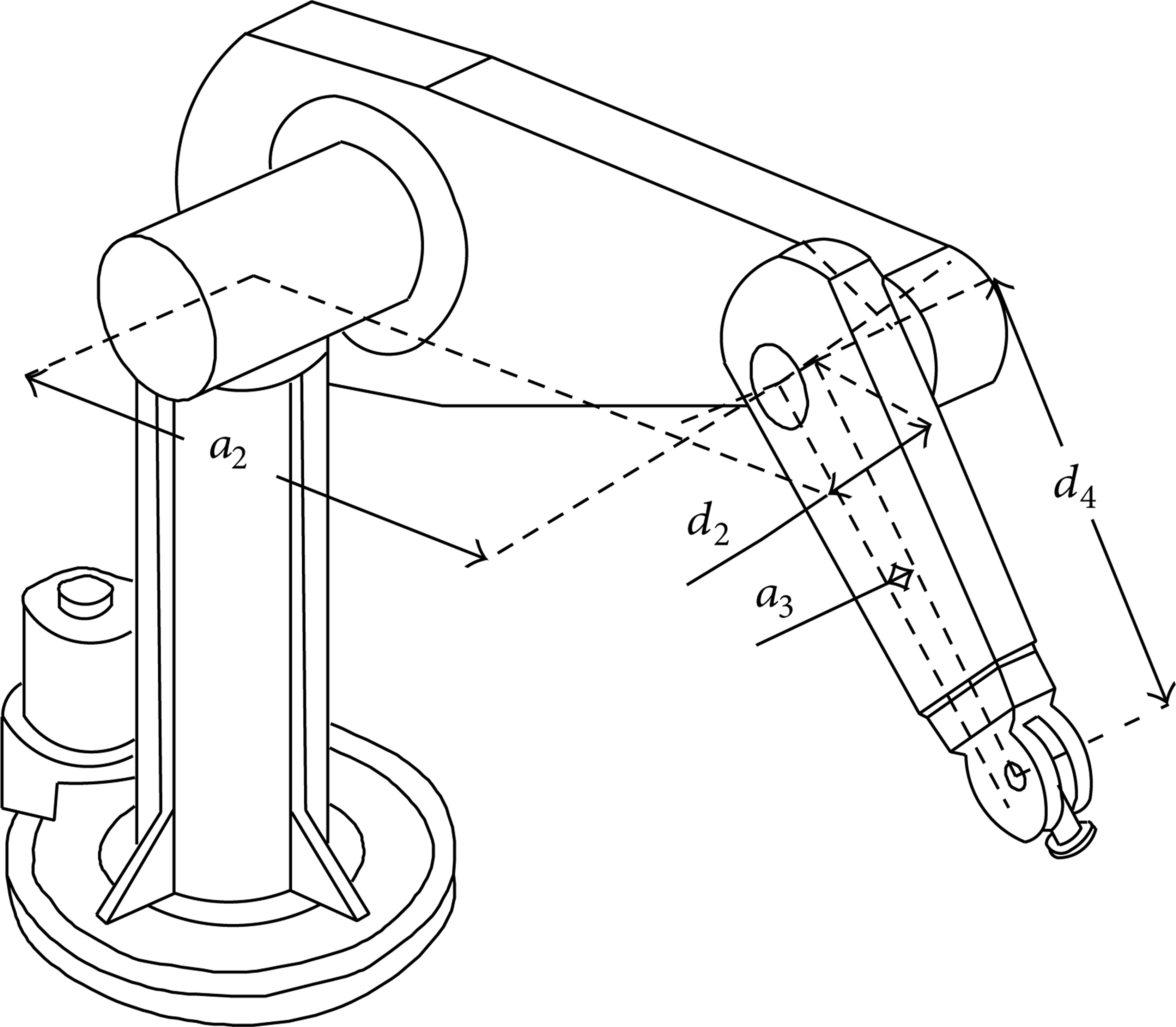
The PUMA 560 robot.

The corresponding geodesic is determined by (3) and (4). Equation (3) corresponding to the Riemannian metric e is a 2-order differential equation group with 3 unknowns (θ₁, θ₂, and θ₃). The geodesic is identified by given initial conditions or boundary conditions.

When the values of θ₁, θ₂, and θ₃ are obtained, the orientation depends on θ₄, θ₅, and θ₆ which are selected as local coordinates of the orientation space. Define the Riemannian metric h of the orientation space as follows:

$\begin{array}{c}h={\left(dn\right)}^{\mathrm{2}}+{\left(do\right)}^{\mathrm{2}}+{\left(da\right)}^{\mathrm{2}}\hfill \\ \hspace{0.17em}=\left(\begin{array}{ccc}d{\theta }_{\mathrm{4}}& d{\theta }_{\mathrm{5}}& d{\theta }_{\mathrm{6}}\end{array}\right)H\left(\begin{array}{c}d{\theta }_{\mathrm{4}}\\ d{\theta }_{\mathrm{5}}\\ d{\theta }_{\mathrm{6}}\end{array}\right),\hfill \end{array}$

(12)

where

$H={\left(h_{ij}\right)}_{\mathrm{3}\times \mathrm{3}}=\left(\begin{array}{ccc}\mathrm{2}& \mathrm{0}& \mathrm{2}{c}_{\mathrm{5}}\\ \mathrm{0}& \mathrm{2}& \mathrm{0}\\ \mathrm{2}{c}_{\mathrm{5}}& \mathrm{0}& \mathrm{2}\end{array}\right)$

(13)

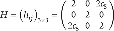
is the coefficient matrix corresponding to h.

Equation (3) corresponding to the Riemannian metric h is a 2-order differential equation group. With the Riemannian metrics e and h, the trajectories can be obtained by solving the geodesic equations under boundary conditions.

For example, when the robot moves linearly from the initial point A to the end point B, the coordinates of A and B are shown in Tables 2 and 3. The robot performs a linear motion from the initial point to the end point according to this planning. The trajectory of the end-effector determined by the geodesic method is shown in Figure 3(a). The velocity, acceleration, and jerk of the end-effector are shown in Figure 3(b). The orientation of the robot end-effector is shown in Figure 4. The joint trajectories are shown in Figure 5. As it can be seen, not only the position trajectories but also the orientation trajectories of the end-effector are smooth. The joint trajectories and their derivatives (velocity, acceleration, and jerk, resp.) are also smooth.

Table 2:

The coordinates of the end points in the Cartesian space.

	A	B
p	(−67, 138, −347) (mm)	(−128, 100, −200) (mm)
n	(−0.6, 0.2, −0.774597)	(−0.4, 0.5, −0.768115)
o	(0.675603, −0.391868, −0.6245)	(0.699733, −0.374666, −0.608276)
a	(−0.428439, −0.89802, 0.1)	(−0.591924, −0.780785, −0.2)

Table 3:

The coordinates of the end points in the joint space.

	A	B
t (s)	0	5
θ1 (rad)	0.214251	0.499461
θ2 (rad)	0.514124	0.549039
θ3 (rad)	0.787751	1.12713
θ4 (rad)	−1.25336	−2.20054
θ5 (rad)	0.975085	0.520477
θ6 (rad)	0.490851	1.50993

Figure 3:

The trajectories of the end-effector according to the linear motion: (a) the positions and (b) the velocities, accelerations, and jerks.

Figure 4:

The orientation of the end-effector.

Figure 5:

The joint trajectories of the PUMA 560 robot.

3.6. Results of the Simulations

The method described in this paper has been tested in simulations for the PUMA 560 robot. The results of the simulations declare that the motion of the robot end-effector is accurate and the trajectories and their derivatives are smooth as shown in Figure 3. The orientation of the end-effector is smooth as shown in Figure 4. The trajectories of the joints and their derivatives are smooth as shown in Figure 5. That is, the method can be used to plan smooth and accurate motions of end-effectors and corresponding smooth joint trajectories for industrial robots.

4. Conclusion and Future Work

A smooth and accurate trajectory planning for industrial robots using geodesics is presented in this paper. The main idea is to select a suitable metric for which a geodesic is the desired motion. The workspace of a robot is split into positional and orientational parts. A Riemannian metric is given on each space such that the desired motion is a geodesic. The geodesic equations are solved numerically and the results are used to control the robot. Simulations of this method using the PUMA 560 robot are given.

The method applies to robots with no more than 6 DOFs and focuses on linear motions. Future work will be directed towards constructing appropriate metrics to plan trajectories of robots with more than six or redundant DOFs and achieve geodesic planning of circular and other curve motions.

Conflict of Interests

The authors declare that there is no conflict of interests regarding the publication of this paper.