Sage Journals: Discover world-class research

Abstract

The vibration testing of components in the automotive industry requires long testing times and the use of expensive facilities. To shorten these testing times an accelerated vibration-testing approach is usually applied. This research tries to shorten these testing times by considering the parameters that define vibration-testing techniques. With special attention to the excitation types sweep-sine and random, a damage-based approach is applied. The phenomenon of fatigue damage is closely observed from the frequency-domain point of view but also by considering the relationship between the time and the frequency domains. The Palmgren-Miner cumulative rule is applied to calculate the fatigue life. Two case studies of measured responses are used to compare the times to failure. The results show that proposed predictions can be used to compare different testing techniques, but they are not so accurate when predicting the actual times to failure.

1. Introduction

The automotive industry's quality requirements often include the vibration testing of parts, which involves long testing times and the use of expensive facilities. An accelerated vibration-testing approach is usually applied to shorten the testing times of the product or quicken the degradation of the product's performance. Three of the most common accelerated test methods are the inverse power-law model [1], the Arrhenius acceleration model [2], and the fatigue-damage model (with Miner's rule) [3]. The most common damage model used to design accelerated durability vibration tests, according to Piersol [4], is the fatigue-damage model.

Fatigue damage can be defined as the modification of the characteristics of a material due to the formation of cracks and resulting from the repeated application of stress cycles that can lead to failure [5].

It is generally accepted that the Rainflow counting method is the most accurate for calculating fatigue damage [6 –8]. The algorithm reduces the spectrum of varying stresses to a set of simple stress reversals and counts the cycles of the applied load in the time history of stress. The method eases the application of the accumulation rule to assess the fatigue life of the structure subjected to complex loading. Different cumulative damage rules are available. The Palmgren-Miner cumulative rule is commonly assumed to be a suitable choice, which presumes that the total life of a part may be estimated by adding up the percentage of the life accumulated by each stress cycle.

In 1964 Bendat [9] introduced a theoretical basis for an approach to damage estimation in the frequency domain. The solution applies to problems with narrow-band responses. Consequently, several methods, discussed later, were developed and Braccessi et al. [10] divided them into three major groups based on spectral moments, distribution functions, and the Rainflow algorithm.

The group of frequency methods based on spectral moments expands the applicability of Bendat's theory [9] with the use of correction factors based on spectral moments. This approach misses the information of load cycles, as it directly computes the damage. In contrast, the second group of methods, based on distribution functions, computes the original probability density function (PDF) of the amplitude cycles, usually with a combination of the common probability density functions (Weibull, Rayleigh, exponential, etc.) [11]. The coefficients of the individual functions depend on the spectral moments and are acquired from measurement data. The most important method in this field is the Dirlik method [12], which produces results comparable to time-domain methods [10, 13]. The third group of methods are based on the Rainflow algorithm. They use a part of the Rainflow counting method algorithm, looking for hysteresis loops in a time history signal and trying to convert them to the frequency domain. These methods have the best theoretical background; however, due to their high numerical demand they are not often used in practice [10].

Since the objective of the frequency-domain approach is also a rapid evaluation of the damage during the first steps of the design, the distribution-functions-based group is closely observed. The stress power spectral density (PSD) represents the frequency-domain input into the fatigue-damage calculations for this group of methods. Many authors [10, 14 –17] focus on the analysis of the particular PSD signal shape, either with one or, more commonly, with two dominant frequencies (bimodal PSD).

The current state of knowledge in the field of frequency-domain methods can be classified on the basis of the bandwidth of the process, dividing them into narrow-band and broad-band processes methods [18, 19]. An overview of the frequency methods was made by Sherratt et al. [7] and recently by Mršnik et al. [13]. The modern methods mostly presume a normal (Gauss) distribution loading. A well-known case is the narrow-band approximation, which produces conservative results for broad-band loadings [10]; therefore, some authors use several correction factors to consider the influence of the bandwidth [18]. The methods from [8, 12, 16, 20] approach the problem with approximations using theoretical simplifications, reductions, or best-fit methods. Benasciutti and Tovo [18] propose a method for random loading, using the loading distribution data from the time-domain methods to consider the bandwidth and distribution in the frequency-domain method.

In this paper we investigate accelerated vibration testing on electrodynamic shakers. The goal is to find the equivalent vibration-test specifications for the sine-sweep and random-excitation techniques and test durations with the same fatigue-damage effect on the tested structure. The phenomenon of fatigue damage is closely observed from the frequency-domain point of view, which requires a detailed investigation of the relationship between the time and the frequency domains.

A consideration of the excitation testing parameters in fatigue-damage calculations is usually missing in the methods covering the field. The presented approach is from here on referred to as the vibration-testing-parameters (VTP) method. The name arises from the use of vibration-testing parameters for balancing the fatigue damage of structures, excited with two different vibration excitations types. The theoretical background of the method is presented in Section 2, which is divided into three subsections that present the random-excitation approach, the sweep-sine-excitation approach, and the joined calculation of vibration-fatigue damage. Two case studies of the vibration-testing-parameters method are presented in Section 3, accompanied by a description of the experiment. The conclusions are discussed in Section 4.

2. Theoretical Background

Vibration-testing techniques use the concept of forced vibration to control the excitation of the structure with a specified dynamic loading. Our focus is on the vibration-testing excitation applied with an electrodynamic shaker. This provides a controlled environment with an arbitrary excitation control over a wide range of parameters [21, 22]. In this section, two main concepts of vibration excitation and its responses are considered: the sweep-sine excitation and the random excitation, each in its own subsection. For each excitation type a method for obtaining the response amplitude in dependence on number of cycles A(n) in described. In the last subsection a joined calculation of vibration-fatigue damage is presented for both types of vibration excitation.

2.1. Sweep-Sine-Excitation Frequency Response

Sweep-sine vibration testing is a widely used type of sine testing excitation. With a change of the excitation frequency, the frequency range of interest is covered. The sweep-sine can be defined with a linear or logarithmic dependency of the frequency over time.

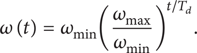
Sinusoidal broad-band excitation is obtained by varying the frequency ω(t) of the sine wave over time:

u (t) = a \sin (ω (t) t + ϕ) .

(1)

The excitation amplitude a and the phase φ are constants, while the angular frequency ω(t) is a function of time. In our case, the logarithmic dependency will be observed. It is defined as in (2), where T_d is the duration of the time signal, and ω_{min ⁡} and ω_{max ⁡} are the lower and upper limits of the frequency range of interest. Consider

ω (t) = ω_{\min} {(\frac{ω_{\max}}{ω_{\min}})}^{t / T_{d}} .

(2)

Equation (2) only provides information about the frequency at a specific time, missing the time that the signal spent at that frequency. This is crucial information for defining the number of cycles of a certain amplitude that is applied to the structure. The speed of the sweep, also known as the sweep rate v_s, defines the speed of the signal passing the frequency range of interest, typically in units of octaves per minute. From the definition of the octave [23], the time t(ω) spent at the frequency of interest is derived and the time spent at an arbitrary frequency is defined as the differential of the time versus the frequency; see (4). Consider

t (ω) = \frac{1}{v_{s}} \frac{\log (ω / ω_{\min})}{\log (2)},

(3)

\frac{d t (ω)}{d ω} = \frac{1}{v_{s} \log (2)} \cdot \frac{1}{ω} .

(4)

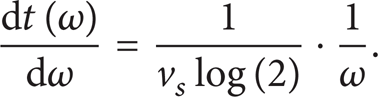
(The derivation can also be computed from the definition of the decade, changing the factor log(2) to log(10). The choice of the base used is made on the basis of the unit of the sweep rate used in defining the vibration-testing excitation parameters.) To define the number of cycles at an arbitrary frequency, the time spent at that frequency is multiplied by the frequency itself:

n_{i} = ω \cdot \frac{d t (ω)}{d ω} = \frac{1}{v_{s} \log (2)} .

(5)

Evidently, the number of cycles of the sinusoidal sweep excitation is constant through the frequency range of interest, meaning that the structure is excited and responds with the same number of cycles for all amplitudes. The stress amplitude A of the structure response to acceleration amplitude a of the applied excitation is obtained either with numerical simulation or, as in our case, experimentally by measuring the structure strain response spectra. All the individual stress response amplitudes A with the computed number of cycles n in the form of A(n) are used to calculate the damage, as described later in Section 2.3.

2.2. Random-Excitation Frequency Response

A random vibration is neither deterministic nor periodic; therefore obtained structural response is mostly treated using statistical or probabilistic approaches. Random vibration signals in the frequency domain are commonly presented as power spectral density (PSD) functions. For the excitation of real structures a broad-band excitation is used to cover a wide range of random effects [24, 25].

Since our final interest is in a fatigue-damage calculation based on an amplitude spectrum, the relationship between the time-domain signal's amplitude and the frequency-domain PSD function is here researched in detail.

The PSD of a stationary discrete random process S_yy(ω) is defined as a time-discrete Fourier transform of the autocorrelated sequence R_xx(t) of a random response. Consider

S_{y y} (ω) = \frac{1}{2 π} \sum_{t = - \infty}^{\infty} ‍ R_{x x} (t) \cdot e^{- i ω t} .

(6)

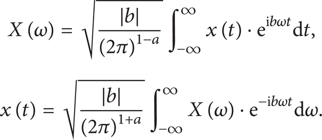
The transformation of a function, signal, or response from the time to the frequency domain with a Fourier transform depends on the shape and the properties of the signal itself. In different areas of science, a number of different normalizations are in use [26]. In general, the forward and inverse Fourier transform pair may be defined using two constants, a and b, in (7). Different selections for these two constants produce different normalizations of the Fourier transform. Typical pairs of values are {a, b} = {0, − 2π} or {1,1} or {0,1} [26]. Consider

\begin{matrix} X (ω) = \sqrt{\frac{|b|}{{(2 π)}^{1 - a}}} \int_{- \infty}^{\infty} ‍ x (t) \cdot e^{i b ω t} d t, \\ x (t) = \sqrt{\frac{|b|}{{(2 π)}^{1 + a}}} \int_{- \infty}^{\infty} ‍ X (ω) \cdot e^{- i b ω t} d ω . \end{matrix}

(7)

To research a real structure response function, a simple mass-spring model of a dynamic system is introduced as one-degree-of-freedom system. Its time response is a continuous cosine function defined as in (8), where the phase of the frequency response was set to zero (ϕ = 0) for the sake of clarity. Consider

x (t) = A \cos (ω t + φ) .

(8)

Integration limits that are different to the period of the integrated trigonometric function produce the transformation results in a complex form. A nonzero imaginary component results in a nonzero phase response, which is in contradiction with our assumption. To avoid the nonzero imaginary component, the fundamental period of the response function of this model is used as the integration limit: T₀ = 2π/ω.

To cover longer time responses the transformation must be normalised with 1/n, where the integer n is the quotient between the length of the time response (full integration range) and the fundamental period length. The integration limits must also be appropriately scaled, to cover the time range of the responses.

By considering all the assumptions stated above, the generalized Fourier transform for a simple model of a dynamic system is

X (ω) = \sqrt{\frac{|b|}{{(2 π)}^{1 - a}}} \frac{1}{n} \int_{0}^{(2 π / ω) n} ‍ x (t) \cdot e^{- i b ω t} d t .

(9)

With (9) set, the time response of the one-degree-of-freedom system from (8) is considered. The result of the transformation is presented in extended form to allow different normalizations of the Fourier transform to be considered (with an appropriate choice of a and b) in

X (ω) = \sqrt{\frac{|b|}{{(2 π)}^{1 - a}}} \frac{A}{(b^{2} - 1) n ω} \cdot i \cdot (- b + e^{- 2 i b n π} (b \cos (2 n π) + i \sin (2 n π))) .

(10)

The normalizations of the Fourier transform that result from the value b = ± 1 have to be considered separately, as the introduction of this value in the result of (10) leads to complex infinity. To avoid this situation, the value b = ± 1 is introduced before the transformation takes place.

Since the assumption of n as an integer, the result of (10) further simplifies to (11), considering the time-response duration, defined as a multiple of the fundamental period of the system's oscillation. Consider

X (ω) = \sqrt{\frac{1}{{(2 π)}^{1 - a}}} \frac{A π}{ω} .

(11)

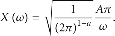
The frequency response computed in (11) is often referred to as an amplitude spectrum. For a known amplitude spectrum (e.g., from a measurement), the amplitude of the oscillation can be computed:

A = (\frac{ω}{π} \sqrt{{(2 π)}^{1 - a}}) X (ω) .

(12)

As mentioned previously, a common quantity to represent the frequency characteristics is the power spectral density function PSD(ω). For a continuous amplitude spectrum function X(ω), the PSD is defined as in [24]:

PSD (ω) = \frac{X (ω) X {(ω)}^{*}}{T} = \frac{X (ω) X {(ω)}^{*}}{n (2 π / ω)} = \frac{1}{{(2 π)}^{1 - a}} \frac{A^{2} π}{2 n ω} .

(13)

From (10) the amplitude of the oscillation can be computed:

A = \sqrt{\frac{2 n ω}{π} {(2 π)}^{1 - a} PSD (ω)} .

(14)

The amplitude spectra of the response to a random excitation are computed from (14). The application of random vibration to the structure excites all the frequency range simultaneously. The frequency is the number of occurrences of a repeating event per unit of time. Number of cycles at each frequency is computed by multiplying each frequency with the duration of the measurement. The computed value is then assigned to the associated response amplitude, in the form of an inverse function, as an amplitude-versus-cycles plot. This result is then used to calculate the vibration-fatigue damage.

2.3. Calculation of Vibration-Fatigue Damage

In the previous two sections the path from the frequency measured response to the computation of the amplitude versus number of cycles data was discussed. The derivation depends on the vibration-testing excitation applied. In this section the calculation of the vibration-fatigue damage from the amplitude versus cycles is explained for both types of vibration excitation.

The definition of the number of cycles n_i for a specific stress amplitude S_i during a period of time T_d from [17] is

n_{i} = n (S_{i}) = E [P] \cdot T_{d} \cdot p_{p} (S_{i}),

(15)

where E[P] is the expected number of peaks per unit of time and p_p(S_i) is the probability density function (PDF) of the stress peaks.

Newland [25] used the definition of the number of cycles from (15) with Miner's rule to calculate the accumulated fatigue damage D:

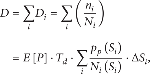
D = \sum_{i} ‍ D_{i} = \sum_{i} ‍ (\frac{n_{i}}{N_{i}}) = E [P] \cdot T_{d} \cdot \sum_{i} ‍ \frac{p_{p} (S_{i})}{N_{i} (S_{i})} \cdot Δ S_{i},

(16)

where N_i(S_i) is the dependency of the number of cycles to fracture of the individual stress amplitude, defined by the material parameters obtained from the Woehler curve. The parameters used are the S-N curve slope and its intercept at 1 cycle. The methodology for obtaining these parameters relatively quickly was proposed by Česnik et al. [27, 28]. The probability density function (PDF) of the stress peaks p_p(S_i) describes the statistical variability of the stress peaks and is often presented as the curve over the histogram of the event distribution.

The formulation in (15) was adopted from Tovo [8] with the assumption that the damage may be related to peak distribution p_p because its positive part agrees with the amplitude distribution p_a. Since both distributions relate only for narrow-band processes, an over-conservative estimate of fatigue damage is expected. Therefore, calculated fatigue damage is here used as a comparison parameter between three p_a calculation approaches and between vibration excitation techniques and not as a measure of actual fatigue damage.

In the vibration-testing-parameters (VTP) method, the PDF of the amplitude of structure response was obtained by interpolating the function over the amplitude-versus-cycles histogram. The interpolation was made by fitting 3rd order polynomial curves between successive data points in the amplitude-versus-cycles data.

Beside the described approach, the Rayleigh p_r(S) [14] and Dirlik p_d(S) [12] PDF of the cycle amplitude S definitions were also considered:

\begin{matrix} p_{r} (S) = \frac{S}{m_{0}} \cdot e^{- (S^{2} / 2 m_{0})}, \\ p_{d} (S) = \frac{1}{{\sqrt{m}}_{0}} \cdot (\frac{D_{1}}{Q} e^{- Z / Q} + \frac{D_{2} Z}{R^{2}} e^{- Z^{2} / 2 R^{2}} + D_{3} Z e^{- Z^{2} / 2}), \end{matrix}

(17)

where

\begin{matrix} Z = \frac{S}{\sqrt{m_{0}}}, x_{m} = \frac{m_{1}}{m_{0}} \cdot \sqrt{\frac{m_{2}}{m_{4}}}, \\ D_{1} = \frac{2 (x_{m} - m_{2}^{2})}{1 + m_{2}^{2}}, \\ D_{2} = \frac{1 - m_{2} - D_{1} + D_{1}^{2}}{1 - R}, \\ D_{3} = 1 - D_{1} - D_{2}, \\ Q = \frac{1.25 (m_{2} - D_{3} - D_{2} R)}{D_{1}}, \\ R = \frac{m_{2} - x_{m} - D_{1}^{2}}{1 - m_{2} - D_{1} + D_{1}^{2}} . \end{matrix}

(18)

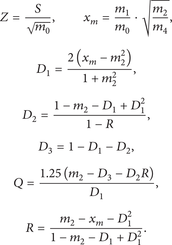
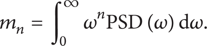
The values m₀, m₁, m₂, and m₄ are the spectral moments obtained from (19), considering the corresponding number for the index n. Consider

m_{n} = \int_{0}^{\infty} ‍ ω^{n} PSD (ω) d ω .

(19)

For sine-sweep excited structures, the application of narrow-band solutions is usually more appropriate, but according to Sherratt et al. [7], the Dirlik method shows good applicability to both narrow- and broad-band signals.

From the obtained PDF function, the damage for both types of vibration excitation was calculated in frequency domain, following the idea of Miner's damage-accumulation rule; see (16). Based on these values, both vibration-excitation types can be compared. The excitation levels for vibration testing are then changed with varying of vibration-testing parameters, until achieving comparable fatigue-damage results for each vibration excitation type.

3. Case Studies

The experimental evaluation of the proposed idea was tested on two different structures. The first was a laboratory experiment of a simple structure, a clamped beam. The second case was a field experiment on a more complex structure, an alternator front bracket.

For both experimental cases the measurement set-up is shown in Figure 1. Each structure was dynamically excited with an LDS V875 electrodynamic shaker (Figure 2), applying the two main concepts of the vibration excitation: the sweep-sine excitation and the random excitation.

Figure 1:

Measurement set-up.

Figure 2:

LDS V875 electrodynamic shaker.

The response-strain spectra to a unit random and a unit sweep-sine excitation are measured for both structures. The acceleration response spectra were measured with piezoelectric integrated electronic accelerometers (IEPE tri-axial B&K4520) to control the changes in the structure. All the responses were recorded in the frequency range between 20 and 2000 Hz, with a sampling frequency of 6400 Hz, a frequency resolution of 2 Hz for the random excitation, and a variable frequency resolution for the sweep-sine excitation.

The stresses were calculated from the measured strain spectra through linear stress-strain relation with modulus of elasticity. They were used to calculate the vibration-fatigue damage of the applied testing conditions with (16). The response was then scaled and the damage recalculated to obtain reasonable times for the vibration testing. At the end, all the structures were exposed to accelerated excitation profiles until visual changes were detected on the response spectrum, indicating damage to the structure.

3.1. Laboratory Experiment

As a simple structure, an aluminium block beam (210 mm × 40 mm × 20 mm) with a 16 mm diameter hole close to the clamping was considered (Figure 3). The purpose of the hole is a controlled weakening of the structure in the desired point. The response was measured in the form of a strain spectrum with 1/4 bridge strain gauges of the type HBM-1-LY13-6/120 (6 mm), placed above the point of expected fracture (Figure 4).

Figure 3:

Clamped beam with strain gauge.

Figure 4:

Clamped beam strain PSD response to random excitation.

The measured responses were scaled and then used to calculate the damage for both excitation types, following the equations and procedures described in Section 2.

The calculated damage for a 10-hour sweep-sine excitation with the excitation profile in the range from 50 to 2000 Hz, with the acceleration amplitude of 15 g and a sweep rate of 1 oct/min, is presented in Table 1. Similarly, the damage for the 10-hour random excitation in the range from 20 to 2000 Hz with the PSD acceleration amplitude of 0.114 g²/Hz is also presented in Table 1.

Table 1:

Comparison of calculated damage using different methods for both types of excitations of the clamped beam.

Method	Sweep-sine	Random

Dirlik	5.91·10⁻⁵	1.88·10⁻⁶
Rayleigh	6.38·10⁻⁵	1.98·10⁻⁶
VTP	1.06·10⁻⁶	2.04·10⁻⁸

The beam was then dynamically tested again on the electrodynamic shaker for both types of excitation, this time with the accelerated profile described in the previous paragraph. The change in the response spectrum during the testing indicated the presence of the break (Figure 5).

Figure 5:

Change in the response spectra.

The break was visually examined for each beam and proved with the penetrant-inspection method (Figure 6). The beam excited with the sweep-sine profile broke after 6.5 hours and the beam excited with the random profile broke after 11 hours of testing.

Figure 6:

Crack on the inner surface of the beam hole.

3.2. Field Experiment

The second case study was taken from the automotive field. For the study, an alternator front bracket was clamped like in a real application. A mass in the shape of a cylinder was mounted on the bracket to simulate the mass and the moments of inertia of the alternator's rotor (Figure 7).

Figure 7:

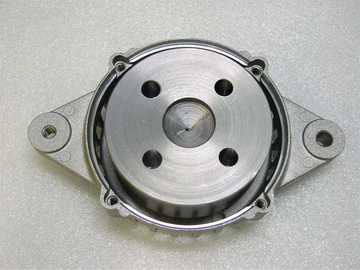
The cylinder mass on the bracket.

The strain-response spectra were measured at the points of the expected fracture with 1/4 bridge strain gauges of the type HBM-1-LY13-3/120 (3 mm) (Figure 8). As in the case of the clamped beam, the measured responses were scaled and used to calculate the damage for both excitation types, following the procedure described in Section 2.

Figure 8:

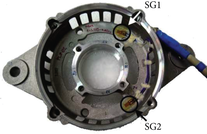
The measurement points on the bracket.

The calculated damage for the 10-hour sweep-sine excitation with the excitation profile in the range from 20 to 2000 Hz with the acceleration amplitude of 10 g and the sweep rate of 2 oct/min is presented in Table 2. In the same table, the calculated damage for the 10-hour random excitation in the range from 20 to 2000 Hz with the PSD acceleration amplitude of 0.0126 g²/Hz is presented.

Table 2:

Comparison of calculated damage using different methods for both types of excitations of the alternator front bracket.

Method	Sweep-sine	Random

Dirlik	7.86·10⁻⁸	5.19·10⁻¹⁶
Rayley	1.12·10⁻⁷	6.74·10⁻¹⁶
VTP	7.60·10⁻⁷	1.40·10⁻¹⁷

The alternator front bracket was then dynamically tested with the accelerated profile for both types of excitation, described in the previous paragraph. The change in the response spectrum indicated the presence of the break (Figure 9).

Figure 9:

Change in the response spectra due to the crack for the sine-sweep (a) and the random excitation (b).

The break was then visually examined and proved with the penetrant-inspection method (Figure 10). The bracket excited with the sweep-sine broke after 1.3 hours and the bracket excited with the random profile broke after 4.8 hours of testing (Figure 11).

Figure 10:

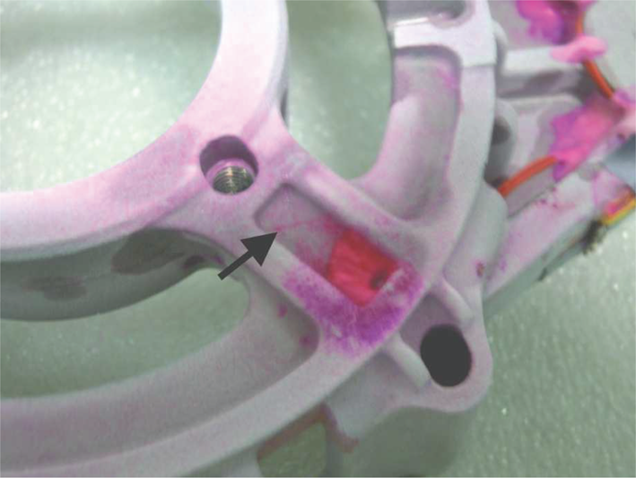
Crack on the bracket proved with the penetrant-inspection method.

Figure 11:

Crack detail on the bracket.

4. Conclusions

In this research, an alternative frequency-domain-based approach for the evaluation of the vibration-fatigue damage was considered for a comparison of two main concepts of vibration-testing excitation techniques.

The vibration-testing-parameters method uses the response amplitudes of an excited structure to estimate the distribution as an interpolation function for the amplitude-versus-cycle data, gathered from the measured-response PSD data. For the two dominant types of vibration excitation, equations for the evaluation of the vibration-fatigue damage were used to accelerate the vibration tests and to compare the excitations.

In two different experimental cases, the excitation techniques sweep-sine and random are used to bring the structure to fracture. Preliminary measurements of the strain spectra for both case studies were made to gather the data for the calculation of the vibration-fatigue damage. The first case structure was a simple clamped beam with an imposed weakening, where the fracture was expected and then actually occurred. The second case studied was an alternator front bracket from production. The fracture location was more difficult to predict in this case, and the measurements of the strain spectra were made at the point of the previous fracture locations reported from the application. The calculated damage for random and sine-sweep testing from Tables 1 and 2 can be compared in terms of severity to the structure. More precisely, the calculated results show that the sweep-sine excitation causes higher damage and is thus more severe. The experimental testing confirms this, as the failure on the structure in both cases studied occurred with the sweep-sine excitation sooner than with the random excitation.

The vibration-testing-parameters method was compared with two generally used approaches for vibration-damage calculations and it showed a relatively good estimation ability. The differences could arise from a consideration of the time to failure when interpolating the PDF function in the vibration-testing-parameters method. The largest difference is in the case of the clamped beam with a random excitation, where the time to failure was the longest. However, the main point of the approach is not to calculate the exact fatigue damage or the actual time to failure but to use it as an estimate to compare different vibration tests on the basis of an actual structural response. In terms of a comparison between the excitation techniques, the method shows good results compared to the other two methods.

Conflict of Interests

The authors declare that there is no conflict of interests regarding the publication of this paper.

References

Allegri

and Zhang

, “On the inverse power laws for accelerated random fatigue testing,” International Journal of Fatigue, vol. 30, no. 6, pp. 967–977, 2008.

Nelson

, Accelerated Testing: Statistical Models, Test Plans, and Data Analysis, John Wiley & Sons, New York, NY, USA, 3rd edition, 1990.

Collins

J. A.

, Failure of Materials in Mechanical Design: Analysis, Prediction, Prevention, John Wiley & Sons, 1993.

Piersol

A. G.

, “Accelerated vibration testing,” Tustin Training News, 1993.

Lalanne

, Mechanical Vibration and Shock Analysis: Fatigue Damage, vol. 4, John Wiley & Sons, New York, NY, USA, 2009.

Bishop

N. W. M.

and Sherratt

, “Theoretical solution for the estimation of “rainflow” ranges from power spectral density data,” Fatigue and Fracture of Engineering Materials and Structures, vol. 13, no. 4, pp. 311–326, 1990.

Sherratt

Bishop

N. W. M.

, and Dirlik

, “Predicting fatigue life from frequency-domain data: current methods,” Journal of the Engineering Integrity Society, vol. 18, pp. 12–16, 2005.

Tovo

, “Cycle distribution and fatigue damage under broad-band random loading,” International Journal of Fatigue, vol. 24, no. 11, pp. 1137–1147, 2002.

Bendat

J. S.

, “Probability functions for random responses, prediction of peaks, fatigue damage and catastrophic failures,” Tech. Rep., NASA, Report Prepared under Contract No. NAS-5-4590 by Measurement Analysis Corporation, Los Angeles, Calif, USA, 1964.

10.

Braccesi

Cianetti

Lori

, and Pioli

, “Fatigue behaviour analysis of mechanical components subject to random bimodal stress process: frequency domain approach,” International Journal of Fatigue, vol. 27, no. 4, pp. 335–345, 2005.

11.

Tovo

, “Damage-based evaluation of probability density distribution for rain-flow ranges from random processes,” International Journal of Fatigue, vol. 22, no. 5, pp. 425–429,2000.

12.

Dirlik

, Application of computers to fatigue analysis [Ph.D. thesis], The University of Warwick, 1985.

13.

Mršnik

Slavič

, and Boltežar

, “Frequency-domain methods for a vibration-fatigue-life estimation—application to real data,” International Journal of Fatigue, vol. 47, pp. 8–17, 2013.

14.

Benasciutti

and Tovo

, “On fatigue damage assessment in bimodal random processes,” International Journal of Fatigue, vol. 29, no. 2, pp. 232–244, 2007.

15.

Benasciutti

, Fatigue analysis of random loadings [Ph.D. thesis], Graduate School in Civil and Industrial Engineering, Department of Engineering, University of Ferrara, 2004.

16.

Benasciutti

and Tovo

, “Spectral methods for lifetime prediction under wide-band stationary random processes,” International Journal of Fatigue, vol. 27, no. 8, pp. 867–877, 2005.

17.

T.-T.

and Cebon

, “Predicting fatigue lives for bi-modal stress spectral densities,” International Journal of Fatigue, vol. 22, no. 1, pp. 11–21, 2000.

18.

Benasciutti

and Tovo

, “Fatigue life assessment in non-Gaussian random loadings,” International Journal of Fatigue, vol. 28, no. 7, pp. 733–746, 2006.

19.

Sarkani

Michaelov

Kihl

D. P.

, and Beach

J. E.

, “Fatigue of welded steel joints under wideband loadings,” Probabilistic Engineering Mechanics, vol. 11, no. 4, pp. 221–227, 1996.

20.

Petrucci

and Zuccarello

, “Fatigue life prediction under wide band random loading,” Fatigue and Fracture of Engineering Materials and Structures, vol. 27, no. 12, pp. 1183–1195, 2004.

21.

Ewins

D. J.

, Modal Testing: Theory and Practice, John Wiley & Sons, 2nd edition, 1984.

22.

McConnell

K. G.

, Vibration Testing, Theory and Practice, John Wiley & Sons, 1995.

23.

Norton

M. P.

and Karczub

D. G.

, Fundamentals of Noise and Vibration Analysis for Engineers, Cambridge University Press, 2nd edition, 2003.

24.

Maia

N. M. M.

Silva

J. M. M.

, Theoretical and Experimental Modal Analysis, John Wiley & Sons, Research Studies Press, 1997.

25.

Newland

D. E.

, An Introduction to Random Vibrations, Spectral and Wavelet Analysis, Longman, 3rd edition, 1997.

26.

Weisstein

E. W.

, “Fourier transform,” From Math World—A Wolfram Web Resource, 2014, http://mathworld.wolfram.com/FourierTransform.html.

27.

Česnik

Slavić

, and Boltežar

, “Uninterrupted and accelerated vibrational fatigue testing with simultaneous monitoring of the natural frequency and damping,” Journal of Sound and Vibration, vol. 331, no. 24, pp. 5370–5382, 2012.

28.

Cesnik

and Slavic

, “Vibrational fatigue and structural dynamics for harmonic and random loads,” Journal of Mechanical Engineering, vol. 60, pp. 339–348, 2014.

Fatigue Damage for Sweep-Sine and Random Accelerated Vibration Testing

Abstract

1. Introduction

2. Theoretical Background

2.1. Sweep-Sine-Excitation Frequency Response

2.2. Random-Excitation Frequency Response

2.3. Calculation of Vibration-Fatigue Damage

3. Case Studies

3.1. Laboratory Experiment

3.2. Field Experiment

4. Conclusions

Conflict of Interests

References