Sage Journals: Discover world-class research

Abstract

A simple semitheoretical method for calculating two-phase frictional pressure gradient in horizontal circular pipes using asymptotic analysis to develop a robust compact model is presented. Two-phase frictional pressure gradient is expressed in terms of the asymptotic single-phase frictional pressure gradients for liquid and gas flowing alone. The proposed model can be transformed into either a two-phase frictional multiplier for liquid flowing alone (ϕ_l²) or two-phase frictional multiplier for gas flowing alone (ϕ_g²) as a function of the Lockhart-Martinelli parameter, X. Single-phase friction factors are calculated using the Churchill model which allows for prediction over the full range of laminar-transition-turbulent regions and allows for pipe roughness effects. The proposed model is compared against published data to show the asymptotic behavior. Comparison with other existing correlations for two-phase frictional pressure gradient such as the Chisholm correlation, the Friedel correlation, and the Müller-Steinhagen and Heck correlation, is also presented. Comparison with experimental data for both ϕ_l and ϕ_l versus X is also presented. At the end of the paper, the present asymptotic model is also extended to minichannels and microchannels.

1. Introduction

In the present study, new two-phase flow modeling is proposed, based upon an asymptotic modeling method to overcome the disadvantages of the separate cylinders model of two-phase flow where the liquid and gas phases are assumed to flow independently of each other in two separate parallel circular cylinders. The separate cylinders model of two-phase flow was introduced first by Turner [1]. Since then, it had appeared in a number of texts such as those by Wallis [2], Carey [3], and Brennen [4]. The equations of ϕ_l² and ϕ_g² are [5, see Appendix A]

ϕ_{l}^{2} = {[1 + {(ϕ_{l}^{2})}^{2 (m - n) / ((5 - m) (5 - n))} {(\frac{1}{X^{2}})}^{2 / (5 - n)}]}^{(5 - m) / 2},

(1)

ϕ_{g}^{2} = {[1 + {(ϕ_{g}^{2})}^{2 (n - m) / ((5 - m) (5 - n))} {(X^{2})}^{2 / (5 - m)}]}^{(5 - n) / 2} .

(2)

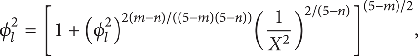
This general form of ϕ_l² in (1) and ϕ_g² in (2) has five different conditions as follows.

m = n = 0.25. This represents turbulent liquid-turbulent gas flow type (Re_l > 2000 and Re_g > 2000).

m = 1, n = 0.25. This represents laminar liquid-turbulent gas flow type (Re_l < 2000 and Re_g > 2000).

m = 0.25, n = 1. This represents turbulent liquid-laminar gas flow type (Re_l > 2000 and Re_g < 2000).

m = n = 1. This represents laminar liquid-laminar gas flow type (Re_l < 2000 and Re_g < 2000).

m = n = 0. This represents constant friction factor liquid-gas flow type.

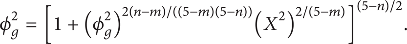
Table 1 shows the expressions of ϕ_l² and ϕ_g² for different flow conditions, respectively.

Table 1:

Expressions of ϕ_l² and ϕ_g² for different flow conditions.

Liquid	Gas	ϕ_l²	ϕ_g²

Turbulent m = 0.25	Turbulent n = 0.25	$ϕ_{l}^{2} = {[1 + {(\frac{1}{X^{2}})}^{1 / 2.375}]}^{2.375}$	$ϕ_{g}^{2} = {[1 + {(X^{2})}^{1 / 2.375}]}^{2.375}$
Laminar m = 1	Turbulent n = 0.25	$ϕ_{l}^{2} = {[1 + {(ϕ_{l}^{2})}^{(3 / 38)} {(\frac{1}{X^{2}})}^{1 / 2.375}]}^{2}$	$ϕ_{g}^{2} = {[1 + {(ϕ_{g}^{2})}^{(- 3 / 38)} {(X^{2})}^{0.5}]}^{2.375}$
Turbulent m = 0.25	Laminar n = 1	$ϕ_{l}^{2} = {[1 + {(ϕ_{l}^{2})}^{(- 3 / 38)} {(\frac{1}{X^{2}})}^{0.5}]}^{2.375}$	$ϕ_{g}^{2} = {[1 + {(ϕ_{g}^{2})}^{(3 / 38)} {(X^{2})}^{(1 / 2.375)}]}^{2}$
Laminar m = 1	Laminar n = 1	$ϕ_{l}^{2} = {[1 + {(\frac{1}{X^{2}})}^{0.5}]}^{2}$	$ϕ_{g}^{2} = {[1 + {(X^{2})}^{0.5}]}^{2}$
f = constant m = n = 0		$ϕ_{l}^{2} = {[1 + {(\frac{1}{X^{2}})}^{0.4}]}^{2.5}$	$ϕ_{g}^{2} = {[1 + {(X^{2})}^{0.4}]}^{2.5}$

From Table 1, it is clear that the expressions of ϕ_l² and ϕ_g² are implicit for liquid-gas laminar-turbulent flow or turbulent-laminar flow. These implicit expressions can be solved by means of computer algebra systems like Maple software [6]. The authors confirm that that there is not any financial gain related to writing Maple software as [6] in the present paper.

The main disadvantage of the separate cylinders model for two-phase flow is not taking into account the important frictional interactions that occur at the interface between liquid and gas, and, needless to say, it would simply neglect the nature of two-phase flow because the liquid and gas phases are assumed to flow independently of each other in two separate parallel circular cylinders. Also, the values of the Reynolds number for the liquid and gas phases are important because these values determine the flow condition and hence the suitable expression for this flow condition. In addition, the obtained expressions are implicit for liquid-gas laminar-turbulent flow or turbulent-laminar flow [5].

In the current study, two-phase frictional pressure gradient is expressed in terms of the asymptotic single-phase frictional pressure gradients for liquid and gas flowing alone. Asymptotes appear in many engineering problems such as steady and unsteady internal and external conduction, free and forced internal and external convection, fluid flow, and mass transfer. Often, there exists a smooth transition between two asymptotic solutions [7 –10]. This smooth transition indicates that there is no sudden change in slope and no discontinuity within the transition region.

The asymptotic analysis method was first introduced by Churchill and Usagi [7], in 1972. After this time, this method of combining asymptotic solutions proved quite successful in developing models in many applications [10]. Recently, it has been applied to two-phase flow in circular pipes [5, 11], minichannels, and microchannels [5, 12]. Moreover, Awad and Butt have shown that the asymptotic method works well for petroleum industry applications for flows through porous media [13], liquid-liquid flows [14], and flows through fractured media [15].

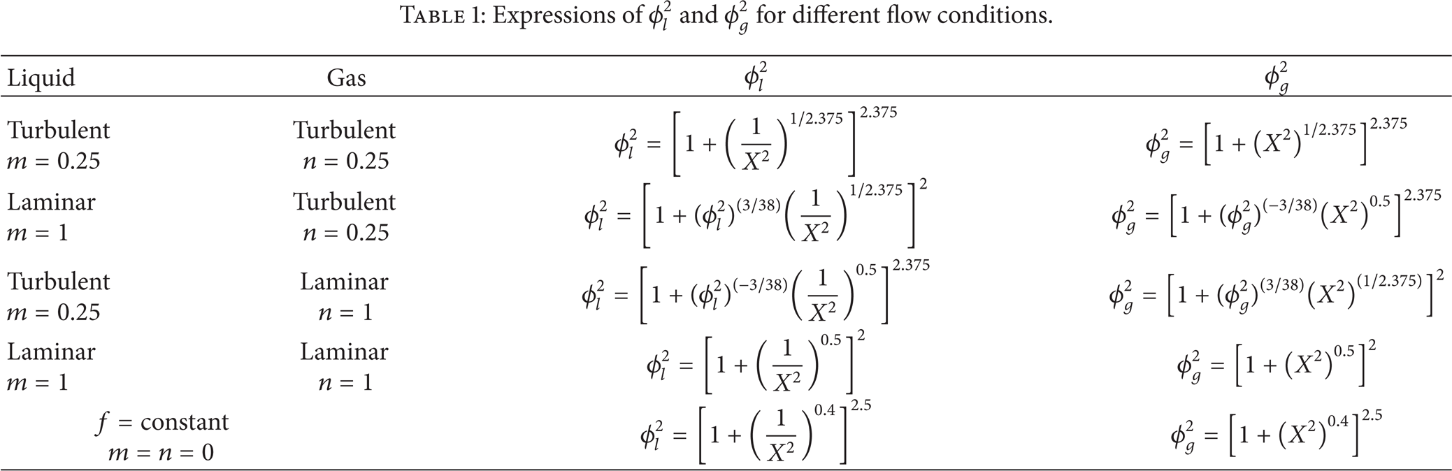
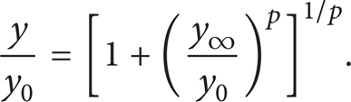
In the asymptotic model, the dependent parameter y has two asymptotes. The first asymptote is y₀, which corresponds to very small value of the independent parameter z. The second asymptote is y_∞, which corresponds to very large value of the independent parameter z. The two asymptotes y₀ and y_∞ can be expressed as follows [7 –10]:

\begin{matrix} y_{0} = c_{0} z^{i}, z ⟶ 0, \\ y_{\infty} = c_{\infty} z^{j}, z ⟶ \infty . \end{matrix}

(3)

The two asymptotes y₀ and y_∞ are based on analytical solution. They consist of a constant, which has a positive real value. The two constants are called c₀ as z → 0 and c_∞ as z → ∞. The values of the two exponents i and j are often 0, 1, 1/2, 1/4, and 1/3 [7 –10].

From analytical, experimental, or numerical methods, it is known that y frequently transitions in a smooth manner between the two asymptotes y₀ and y_∞.

For the case of two-phase frictional pressure gradient in horizontal pipes, the two asymptotes y₀ and y_∞ increase with increasing values of z, and the solution y is concave upwards. This trend is also found in the case of external free and forced convection from single isothermal convex bodies.

Since y₀ > y_∞ as z → 0, so the solution y is concave upwards, and the two asymptotes y₀ and y_∞ can be combined in the following method [7 –10]:

y = {[y_{0}^{p} + y_{\infty}^{p}]}^{1 / p} .

(4)

The parameter p is a fitting or “blending” parameter whose value can be determined in a simple method. The effect of the parameter p in (4) is only important in the transition region. The results for small and large values of the independent parameter z remain unchanged with changing the parameter p.

To determine a value of p, there are a number of methods as discussed by Churchill and Usagi [7]. For example, we can select an intermediate value of z = z_int corresponding or near to the intersection of the two asymptotes for which y(z_int) is known from analytical, experimental, or numerical methods. Using (3) and (4), we can write for the intermediate value of z = z_int,

y (z_{int}) = {[{(c_{0} z_{int}^{i})}^{p} + {(c_{\infty} z_{int}^{j})}^{p}]}^{1 / p} .

(5)

Although the fitting or “blending” parameter p is unknown, it can be calculated by numerical methods for solving a nonlinear equation or by means of computer algebra systems like Maple release 9 software [6].

In the present study, p is chosen as the value, which minimizes the root mean square (RMS) error, e_RMS, between the model predictions and the available data. The fractional error (e) in applying the model to each available data point is defined as

e = | \frac{Predicted - Available}{Available} | .

(6)

For groups of data, the root mean square (RMS) error, e_RMS, is defined as

e_{RMS} = {[\frac{1}{N} \sum_{k = 1}^{N} e_{k}^{2}]}^{1 / 2} .

(7)

If p is a weak function of the mass flow rate, or mass flux of either the liquid phase or the gas phase, a single value may be chosen which best represents all of the available data for two-phase frictional pressure gradient.

The approximate solution y is often presented in a form, which is based on one of the two asymptotes y₀ and y_∞. For example, if the approximate solution y is presented in terms of the asymptote y₀, then the model can be expressed as follows [7 –10]:

\frac{y}{y_{0}} = {[1 + {(\frac{y_{\infty}}{y_{0}})}^{p}]}^{1 / p} .

(8)

On the other hand, if the approximate solution y is presented in terms of the asymptote y_∞, then the model can be expressed as follows [7 –10]:

\frac{y}{y_{\infty}} = {[1 + {(\frac{y_{0}}{y_{\infty}})}^{p}]}^{1 / p} .

(9)

1.1. Asymptotic Modeling in Two-Phase Flow

Using the asymptotic analysis method, two-phase frictional pressure gradient ${(d p / d z)}_{f}$ can be expressed in terms of single-phase frictional pressure gradient for liquid flowing alone ${(d p / d z)}_{f, l}$ and single-phase frictional pressure gradient for gas flowing alone ${(d p / d z)}_{f, g}$ as follows:

{(\frac{d p}{d z})}_{f} = {[{(\frac{d p}{d z})}_{f, l}^{p} + {(\frac{d p}{d z})}_{f, g}^{p}]}^{1 / p} .

(10)

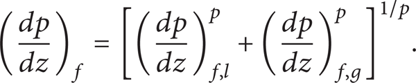
Equation (10) reduces to ${(d p / d z)}_{f, l}$ and ${(d p / d z)}_{f, g}$ as x = 0 and 1, respectively. It is clear that the asymptotic analysis method arrives at the same form as the separate cylinders model formulation [1], but with a different physical approach. Rather than modeling the fluid as two distinct fluid streams flowing in separate pipes, the two-phase frictional pressure gradient can be predicted using a nonlinear superposition of the component pressure gradients that would arise from each stream flowing alone in the same pipe, through application of the Churchill-Usagi asymptotic correlation method [7]. This form was asymptotically correct for either phase as the mass quality varied from 0 < x < 1. Further, rather than approaching the Lockhart-Martinelli parameter from the point of view of the four flow regimes using simple friction models, the asymptotic analysis method uses the Churchill [16] model for the friction factor in smooth and rough pipes for all values of the Reynolds number. In this way the proposed model was most general and contained only one empirical coefficient, the Churchill-Usagi [7] blending parameter.

The principal advantages of the asymptotic analysis method over the separate cylinders model formulation [1] are twofold. First, all four Lockhart-Martinelli flow regimes can be handled with ease, since the separate cylinders model formulation [1] leads to implicit relationships for the two mixed regimes. Second, since the friction model used is only a function of Reynolds number and roughness, broader applications involving rough pipes can be easily modeled.

If the two-phase frictional pressure gradient ${(d p / d z)}_{f}$ is presented in terms of the single-phase frictional pressure gradient for liquid flowing alone ${(d p / d z)}_{f, l}$ , then the model can be expressed using the Lockhart-Martinelli parameter (X) as follows:

{(\frac{d p}{d z})}_{f} = {(\frac{d p}{d z})}_{f, l} {[1 + {(\frac{1}{X^{2}})}^{p}]}^{1 / p} .

(11)

Equation (11) can be expressed in terms of a two-phase frictional multiplier liquid flowing alone in the pipe (ϕ_l²) as follows:

ϕ_{l}^{2} = {[1 + {(\frac{1}{X^{2}})}^{p}]}^{1 / p} .

(12)

On the other hand, if the two-phase frictional pressure gradient ${(d p / d z)}_{f}$ is presented in terms of the single-phase frictional pressure gradient for gas flowing alone ${(d p / d z)}_{f, g}$ , then the model can be expressed using the Lockhart-Martinelli parameter (X) as follows:

{(\frac{d p}{d z})}_{f} = {(\frac{d p}{d z})}_{f, g} {[1 + {(X^{2})}^{p}]}^{1 / p} .

(13)

Equation (13) can be expressed in terms of a two-phase frictional multiplier for gas flowing alone in the pipe (ϕ_g²) as follows:

ϕ_{g}^{2} = {[1 + {(X^{2})}^{p}]}^{1 / p} .

(14)

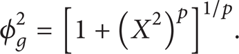
It is clear that (12) and (14) are similar to the separate cylinders model formulation [1] for constant friction factor (1/p = 2.5) or when both liquid and gas are either turbulent (1/p = 2.375) or laminar (1/p = 2). Also, (12) and (14) are still explicit for liquid-gas laminar-turbulent flow and turbulent-laminar flow.

1.1.1. Single-Phase Frictional Pressure Gradient Equations

The single-phase frictional pressure gradient can be related to the Fanning friction factor in terms of mass flow rate of both the liquid phase and the gas phase as follows:

\begin{matrix} {(\frac{d p}{d z})}_{f, l} = \frac{32 f_{l} m_{l}^{2}}{π^{2} d^{5} ρ_{l}}, \\ {(\frac{d p}{d z})}_{f, g} = \frac{32 f_{g} m_{g}^{2}}{π^{2} d^{5} ρ_{g}} . \end{matrix}

(15)

Equation (15) can be written in terms of mass flux and mass quality as follows:

\begin{matrix} {(\frac{d p}{d z})}_{f, l} = \frac{2 f_{l} G^{2} {(1 - x)}^{2}}{{d ρ}_{l}}, \\ {(\frac{d p}{d z})}_{f, g} = \frac{2 f_{g} G^{2} x^{2}}{d ρ_{g}} . \end{matrix}

(16)

The model that was developed by Churchill [16] is introduced to define the Fanning friction factor. When a computer is used, the Churchill model equations [16] are more recommended than the Blasius equations [17] to define the Fanning friction factor [18]. The Churchill model was a correlation of the Moody chart [19]. Churchill's correlation spanned the entire range of laminar, transition, and turbulent flow in pipes. The Churchill model equations that define the Fanning friction factor are

\begin{matrix} f = 2 {[{(\frac{8}{Re})}^{12} + \frac{1}{{(a + b)}^{3 / 2}}]}^{1 / 12}, \\ a = {[2.457 \ln \frac{1}{{(7 / Re)}^{0.9} + (0.27 ε / d)}]}^{16}, \\ b = {(\frac{37530}{Re})}^{16} . \end{matrix}

(17)

The Reynolds number equations can be expressed in terms of mass flow rate of both the liquid phase and the gas phase or mass flux and mass quality as follows:

\begin{matrix} R e_{l} = \frac{4 m_{l}}{{π d μ}_{l}} = \frac{G (1 - x) d}{μ_{l}}, \\ R e_{g} = \frac{4 m_{g}}{{π d μ}_{g}} = \frac{G x d}{μ_{g}} . \end{matrix}

(18)

2. Results and Discussion

Examples of two-phase frictional pressure gradient in horizontal pipes for published data of different pipe diameters are presented to show features of the asymptotes, asymptotic analysis, and the development of simple compact models. At the end of the paper, the present asymptotic model is also extended to minichannels and microchannels.

2.1. Comparison of the Present Asymptotic Model with Data

Figure 1 shows comparison of the present asymptotic model [11] with Dukler's data [20] for air-water flow in a smooth horizontal pipe at d = 2 in. (50.8 mm). The frictional pressure gradient is represented as a function of the liquid mass flow rate on log-log scale for the gas mass flow rate values of 7.8, 23.3, 81.8, 381, and 1103 lb_m/hr (3.54, 10.57, 37.1, 172.82, and 500.32 kg/s), respectively. For the same value of the gas mass flow rate, the frictional pressure gradient increases with increasing liquid mass flow rate. Also, the frictional pressure gradient increases with increasing gas mass flow rate at the same value of the liquid mass flow rate. Equation (10) represents the present asymptotic model [11]. It can be seen that the present model with fitting parameter p = 1/3.9 represents Dukler's data in a successful manner. The root mean square (RMS) error, e_RMS, is equal to 12.11%. The worst agreement is obtained for data points with an absolute error (e) of 23.34%.

Figure 1:

Comparison of the Asymptotic Model with Dukler's Data [20].

Comparison of different models such as Chisholm [21], Chisholm [22], Friedel [23], and Müller-Steinhagen and Heck [24] as well as the present asymptotic model [11] with p = 1/3.9 with Dukler's data [20] is shown in Table 2.

Table 2:

Comparison of different models with Dukler's data [20].

Model	RMS (%)

Chisholm [21]	23.08
Chisholm [22]	63.13
Friedel [23]	83.32
Müller-Steinhagen and Heck [24]	36.20
Asymptotic [11]	12.11

As a brief on these different models, Chisholm [21] developed equations in terms of the Lockhart-Martinelli correlating groups for the friction pressure drop during the flow of gas-liquid or vapor-liquid mixtures in pipes. His theoretical development was different from previous treatments in the method of allowing for the interfacial shear force between the phases. Also, he avoided some of the anomalies occurring in previous “lumped flow.” He gave simplified equations for use in engineering design for both two-phase frictional multiplier for liquid flowing alone in the pipe (ϕ_l²) and two-phase frictional multiplier for gas flowing alone in the pipe (ϕ_g²) as a function of the Chisholm constant (C) and the Lockhart-Martinelli parameter (X). The values of C were dependent on whether the liquid and gas phases were laminar or turbulent flow. The values of C were restricted to mixtures with gas-liquid density ratios corresponding to air-water mixtures at atmospheric pressure. The different values of C are given as C = 20 for turbulent-turbulent flow, C = 12 for laminar liquid-turbulent gas flow, C = 10 for turbulent liquid-laminar gas flow, and C = 5 for laminar-laminar flow. He compared his predicted values using these values of C and his equation with the Lockhart-Martinelli values. He obtained good agreement with the Lockhart-Martinelli empirical curves.

Chisholm [22] showed that his previous equation in [21] for predicting the friction pressure drop during two-phase flow was an unsatisfactory form for use with evaporating flows as ${(d p / d z)}_{f, l}$ , in that case, varied along the flow path. Therefore, he transformed his equation with sufficient accuracy for engineering purposes to an expression for two-phase frictional multiplier for total flow assumed liquid in the pipe (ϕ_lo²) as a function of physical property coefficient (Γ), Chisholm parameter (B), and mass quality (x).

Friedel [23] proposed a method in terms of the multiplier (ϕ_lo²). He developed his correlation and fit it with 25000 data points. The smallest pipe diameter in the Friedel database was 4 mm. His correlation included both the gravity effect by Froude number (Fr) and the effect of surface tension and the total mass flux by Weber number (We). Friedel [23] proposed a method in terms of the multiplier (ϕ_lo²). He developed his correlation and fit it with 25000 data points. The smallest pipe diameter in the Friedel database was 4 mm. His correlation included both the gravity effect by Froude number (Fr), and the effect of surface tension and the total mass flux by Weber number (We).

Müller-Steinhagen and Heck [24] suggested a new correlation for the prediction of frictional pressure drop in two-phase flow ${(d p / d z)}_{f}$ in pipes. Their correlation had an advantage that was simple and more convenient to use than other methods. They developed an equation for the roughly linear increase of the pressure drop with increasing quality (for x < 0.7). In order to cover the full range of flow quality (0 < x < 1), they used the method of superposition (at x = 1, ${(d p / d z)}_{f} = {(d p / d z)}_{f, g o}$ ). It was obvious that their correlation related the frictional pressure gradient in two-phase flow ${(d p / d z)}_{f}$ to the frictional pressure gradient if the total flow assumed liquid in the pipe ${(d p / d z)}_{f, l o}$ , the frictional pressure gradient if the total flow assumed gas in the pipe ${(d p / d z)}_{f, g o}$ , and the mass quality (x). To determine their reliabilities, they checked their correlation and another 14 correlations against a data bank containing 9313 measurements of frictional pressure drop for different fluids, different tube diameters (between 4 and 352 mm), and different flow conditions (horizontal flow, vertical upwards flow, and vertical downwards flow). The data bank containing only measurements with the frictional pressure gradient ${(d p / d z)}_{f}$ was greater than 20 Pa/m to avoid uncertainties due to the scatter of data.

2.2. ϕ_l and ϕ_g versus Lockhart-Martinelli Parameter (X) in Circular Pipes

Figure 2 shows ϕ_l versus Lockhart-Martinelli parameter (X) for turbulent-turbulent flow for different working fluids in a smooth horizontal pipe of different diameters at different conditions using the present asymptotic model and the first six data sets in Table 3. Equation (12) represents the present model with different values of p as shown in Table 3.

Table 3:

Values of the asymptotic parameter (p) in circular pipes at different conditions.

Author	d (mm)	Working fluid	p	e _RMS	${e_{RMS}}^{*}$

Dukler [20]	50.8	Air-Water	1/3.9	12.11%	29.43%
Chisholm [18]	27	Air-Water	1/4	16.73%	38.21%
Govier and Omer [25]	26.06	Air-Water	1/3.9	8.03%	19.87%
Janssen and Kervinen [26]	18.85	Steam	1/2.9	2.44%	12.90%
Hashizume [27]	10	R12	1/3	8.44%	10.80%
Hashizume [27]	10	R22	1/2.8	9.12%	16.68%
Cicchitti et al. [28]	5.1	Steam	1/3.1	8.29%	9.56%
Cheremisinoff and Davis [29]	63.5	Air-Water	1/2.85	14.21%	18.51%

$^{*}$ Calculated at p = 1/3.25.

Figure 2:

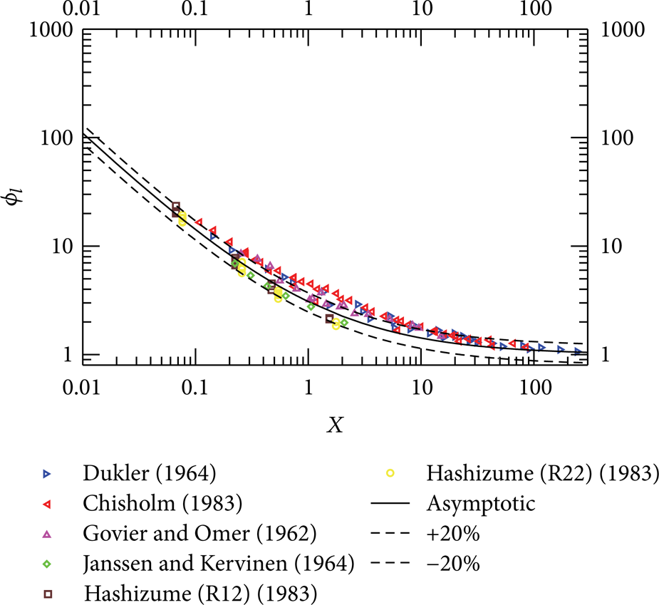
ϕ_l versus X for different sets of data in circular pipes.

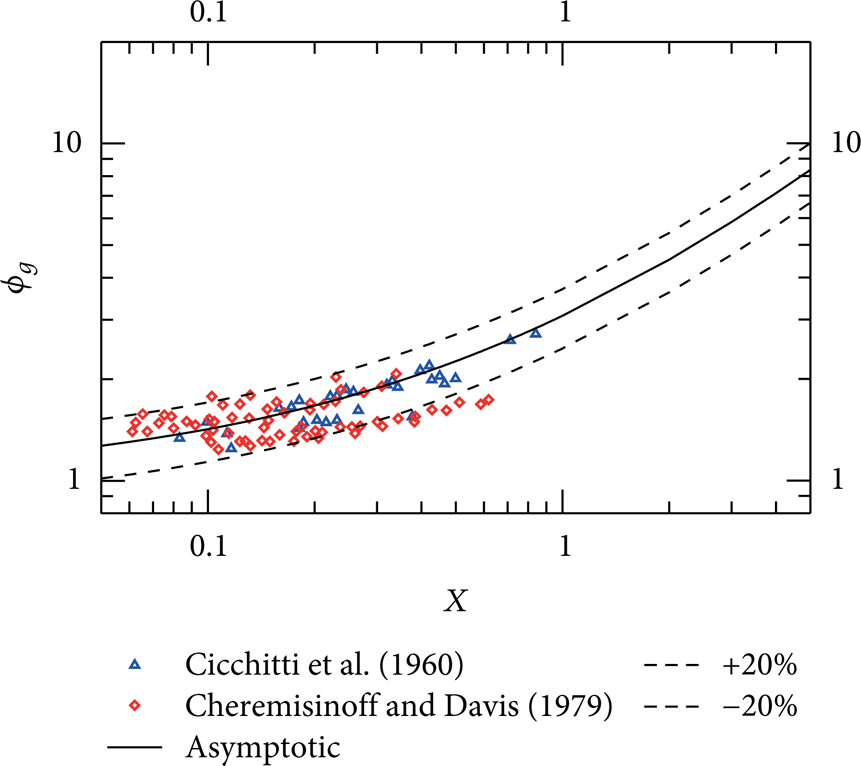
Figure 3 shows ϕ_g versus Lockhart-Martinelli parameter (X) for turbulent-turbulent flow for different working fluids in a smooth horizontal pipe of different diameters at different conditions using the present asymptotic model and the last two data sets in Table 3. Equation (14) represents the present model with different values of p as shown in Table 3.

Figure 3:

ϕ_g versus X for different sets of data in circular pipes.

To have a robust model, one value of the fitting parameter (p) is chosen as p = 1/3.25. When p = 1/3.25, the root mean square (RMS) error e_RMS = 23.80%. Figure 2 shows ϕ_l versus X for the first six data sets in Table 4 while Figure 3 shows ϕ_g versus X for the last two data sets in Table 3 with p = 1/3.25. It can be seen that there is a good agreement between the present asymptotic model and the different data sets in Figures 2 and 3.

Table 4:

Values of the asymptotic parameter (p) in minichannels and microchannels at different conditions.

Author	d (mm)	Working fluid	p	e _RMS	e_RMS at p = 1/2

Ju Lee and Yong Lee [30]	0.78*	Air-Water	1/1.75	11.7%	14.07%
Chung and Kawaji [31]	0.1	Nitrogen-Water	1/1.7	13.44%	16.09%
Kawaji et al. [32]⁺	0.1	Nitrogen-Water	1/2.15	10.39%	11.34%
Kawaji et al. [32]⁺⁺	0.1	Nitrogen-Water	1/2.55	11.65%	17.36%
Ohtake et al. [33]	0.32* 0.42* 0.49*	Argon-Water	1/1.55	19.56% 16.08%**	24.16% 18.24%**

$^{*}$ Hydraulic diameter. $^{* *}$ The two lower points are not taken into account. $^{+}$ Gas in the main channel and liquid in the branch. $^{+ +}$ Liquid in the main channel and gas in the branch.

2.3. ϕ_l and ϕ_g versus Lockhart-Martinelli Parameter (X) in Minichannels and Microchannels

In this section, the present asymptotic model is also extended to minichannels and microchannels using the same published data sets in [34]. Figure 4 shows ϕ_l versus Lockhart-Martinelli parameter (X) for laminar-laminar flow for different working fluids in smooth minichannels and microchannels of different diameters at different conditions using the present asymptotic model and the first three data sets in Table 4. Equation (12) represents the present model with different values of p as shown in Table 4.

Figure 4:

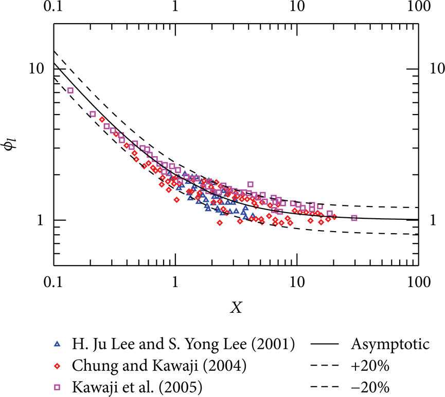
ϕ_l versus X for different sets of data in minichannels and microchannels.

Figure 5 shows ϕ_g versus Lockhart-Martinelli parameter (X) for laminar-laminar flow for different working fluids in smooth minichannels and microchannels at different conditions using the present asymptotic model and the last two data sets in Table 4. Equation (14) represents the present model with different values of p as shown in Table 4.

Figure 5:

ϕ_g versus X for different sets of data in minichannels and microchannels.

To have a robust model, one value of the fitting parameter (p) is chosen as p = 1/2. When p = 1/2, the root mean square (RMS) error, e_RMS = 17.14% or 15.69% if the two lower points of Ohtake et al. data [33] are not taken into account. Figure 4 shows ϕ_l versus X for the first three data sets in Table 4 while Figure 5 shows ϕ_g versus X for the last two data sets in Table 4 with p = 1/2. It can be seen that there is a good agreement between the present asymptotic model and the different data sets in Figures 4 and 5.

3. Summary and Conclusions

New two-phase flow modeling is proposed, based upon an asymptotic modeling method. The main advantage of the asymptotic modeling method in two-phase flow is taking into account the important frictional interactions that occur at the interface between liquid and gas because the liquid and gas phases are assumed to flow dependently of each other in the same pipe. Also, the values of the Reynolds number for the liquid and gas phases are not important because the Churchill model [16] that spanned the entire range of laminar, transition, and turbulent flow in pipes is introduced to define the Fanning friction factor. In addition, the obtained expressions of ϕ_l² and ϕ_g² are explicit for all flow conditions. The only unknown parameter in the asymptotic modeling method in two-phase flow is the fitting parameter (p). The value of the fitting parameter (p) corresponds to the minimum root mean square (RMS) error, e_RMS, for any data set. To have a robust model, one value of the fitting parameter (p) is chosen as p = 1/3.25 for large diameter (macroscale) and p = 1/2 for small diameter (microscale). The difference between the values of p = 1/3.25 for large diameter (macroscale) and p = 1/2 for small diameter (microscale) can be due to the effect of diameter (d) on p.

Footnotes

Appendix

In the appendix, a generalization of the separate cylinders model of two-phase flow will be presented to include laminar liquid-turbulent gas flow and turbulent liquid-laminar gas flow that were not presented in the literature. In the separate cylinders model of two-phase flow, the liquid and gas phases are assumed to flow independently of each other in two separate parallel circular cylinders of radii r_le and r_ge, respectively. The radius of the actual pipe is r_o, and its area is the sum of the area of the separate cylinders.

The gas and liquid volumetric fractions are given as follows:

The pressure over any cross-section of the two-phase flow is assumed to be constant so that the two-phase pressure gradient is the same for each phase. Due to this assumption, the separate cylinders model of two-phase flow is not valid for gas-liquid slug flow that gives rise to large pressure fluctuations [1]. The pressure gradients in the imagined cylinders are therefore both equal to the two-phase frictional pressure gradient in the actual pipe.

The pressure gradient in the separate cylinder of radius r_ge carrying the gas phase is given by

For the gas flowing alone through the actual pipe of radius r_o, the frictional pressure gradient is given by

Using the assumption that the pressure gradient in the imagined cylinder of radius r_ge is equal to the two-phase frictional pressure gradient in the actual pipe of radius r_o and using the definition of ϕ_g², we obtain

The pressure gradient in the separate cylinder of radius r_le carrying the liquid phase is given by

For the liquid flowing alone through the actual pipe of radius r_o, the frictional pressure gradient is given by

Using the assumption that the pressure gradient in the imagined cylinder of radius r_le is equal to the two-phase frictional pressure gradient in the actual pipe of radius r_o and using the definition of ϕ_l², we obtain

Combining (A.4) and (A.7) to eliminate α, we obtain

The definition of X² is given by

Multiplying both sides of (A.8) by ϕ_l^{4/(5 − m)} and using (A.9), we obtain

Multiplying both sides of (A.8) by ϕ_g^{4/(5 − n)} and using (A.9), we obtain

Nomenclature

Conflict of Interests

The authors certify that they have no actual or potential conflict of interests including any financial, personal, or other relationships with other people or organizations within three years of beginning the submitted work that could inappropriately influence, or be perceived to influence, their work.

Acknowledgment

The authors acknowledge the financial support of the Natural Sciences and Engineering Research Council of Canada (NSERC) through the Discovery Grants Program.

References

Turner

J. M.

, Annular two-phaseflow [Ph.D. thesis], Dartmouth College, Hanover, NH, USA, 1966.

Wallis

G. B.

, One-Dimensional Two-Phase Flow, McGraw-Hill Book Company, New York, NY, USA, 1969.

Carey

V. P.

, Liquid-Vapor Phase-Change Phenomena: An Introduction to the Thermophysics of Vaporization and Condensation Processes in Heat Transfer Equipment, chapter 10, Hemisphere Publishing Corporation, Washington, DC, USA, 1992.

Brennen

C. E.

, Fundamentals of Multiphase Flow, chapter 8, Cambridge University Press, Cambridge, UK, 2005.

Awad

M. M.

, Two-phase flow modeling in circular pipes [Ph.D. thesis], Memorial University of Newfoudland, Newfoudland, Canada, 2007.

Maple Release 9, Waterloo Maple Software, Waterloo, Canada, 2003.

Churchill

S. W.

and Usagi

, “A general expression for the correlation of rates of transfer and other phenomena,” American Institute of Chemical Engineers, vol. 18, no. 6, pp. 1121–1128, 1972.

Churchill

S. W.

, Viscous Flows: The Practical Use of Theory, Butterworths, Boston, Mass, USA, 1988.

Kraus

A. D.

and Bar-Cohen

, Thermal Analysis and Control of Electronic Equipment, Hemisphere Publishing Corporation, New York, NY, USA, 1983.

10.

Yovanovich

M. M.

, “Asymptotes and asymptotic analysis for development of compact models for microelectronic cooling,” in Proceedings of the 19th Annual Semiconductor Thermal Measurement and Management Symposium and Exposition (SEMI-THERM '03), San Jose, Calif, USA, 2003.

11.

Awad

M. M.

and Muzychka

Y. S.

, “A simple asymptotic compact model for two-phase frictional pressure gradient in horizontal pipes,” in Proceedings of the ASME International Mechanical Engineering Congress and Exposition (IMECE '04), paper no. IMECE2004-61410, pp. 675–685, Anaheim, Calif, USA, November 2004.

12.

Awad

M. M.

and Muzychka

Y. S.

, “Two-phase flow modeling in microchannels and minichannels,” in Proceedings of the 6th International Conference on Nanochannels, Microchannels, and Minichannels (ICNMM '08), Paper no. ICNMM2008-62134, pp. 299–306, Technische Universitaet of Darmstadt, Darmstadt, Germany, June 2008.

13.

Awad

M. M.

and Butt

S. D.

, “A robust asymptotically based modeling approach for two-phase flow in porous media,” ASME Journal of Heat Transfer, vol. 131, no. 10, Article ID 101014, 12 pages, 2009, Also presented at ASME 27th International Conference on Offshore Mechanics and Arctic Engineering (OMAE '08), Session: Offshore Technology, Petroleum Technology II, OMAE2008-57792, Estoril, Portugal, June 2008.

14.

Awad

M. M.

and Butt

S. D.

, “A robust asymptotically based modeling approach for two-phase liquid-liquid flow in pipes,” in Proceedings of the ASME 28th International Conference on Offshore Mechanics and Arctic Engineering (OMAE '09), paper no. OMAE2009-79072, pp. 409–418, Honolulu, Hawaii, USA, May-June 2009.

15.

Awad

M. M.

and Butt

S. D.

, “A robust asymptotically based modeling approach for two-phase gas-liquid flow in fractures,” in Proceedings of the 12th International Conference on Fracture (ICF '09), paper no. ICF2009646Ottawa, Ottawa, Canada, July 2009.

16.

Churchill

S. W.

, “Friction factor equation spans all fluid flow regimes,” Chemical Engineering, vol. 84, no. 24, pp. 91–92, 1977.

17.

Blasius

, “Das ähnlichkeitsgesetz bei reibungsvorgängen in flüssikeiten,” Forschung auf dem Gebiete des Ingenieurwesens, vol. 131, 1913.

18.

Chisholm

, Two-Phase Flow in Pipelines and Heat Exchangers, George Godwin in Association with Institution of Chemical Engineers, London, UK, 1983.

19.

Moody

L. F.

, “Friction factors for pipe flow,” Transactions of the American Society of Mechanical Engineers, vol. 66, no. 8, pp. 671–677, 1944.

20.

Dukler

A. E.

, “Pressure drop in horizontal conduits,” in Special Summer Program in Two-Phase Gas-Liquid Flow, Griffith

and Gouse

S. W.

Jr. , Eds., Massachusetts Institute of Technology, Cambridge, Mass, USA, 1964.

21.

Chisholm

, “A theoretical basis for the Lockhart-Martinelli correlation for two-phase flow,” International Journal of Heat and Mass Transfer, vol. 10, no. 12, pp. 1767–1778, 1967.

22.

Chisholm

, “Pressure gradients due to friction during the flow of evaporating two-phase mixtures in smooth tubes and channels,” International Journal of Heat and Mass Transfer, vol. 16, no. 2, pp. 347–358, 1973.

23.

Friedel

, “Improved friction pressure drop correlations for horizontal and vertical two phase pipe flow,” in Proceedings of the European Two Phase Flow Group Meeting, paper E2, Ispra, Italy, 1979.

24.

Müller-Steinhagen

and Heck

, “A simple friction pressure drop correlation for two-phase flow in pipes,” Chemical Engineering and Processing, vol. 20, no. 6, pp. 297–308, 1986.

25.

Govier

G. W.

and Omer

M. M.

, “Horizontal pipeline flow of air-water mixtures,” The Canadian Journal of Chemical Engineering, vol. 40, no. 3, pp. 93–104, 1962.

26.

Janssen

and Kervinen

J. A.

, “Two-phase pressure losses,” Final Report GEAP-4634, General Electric Company, San Jose, Calif, USA, 1964.

27.

Hashizume

, “Flow pattern, void fraction and pressure drop of refrigerant two-phase flow in a horizontal pipe. I: experimental data,” International Journal of Multiphase Flow, vol. 9, no. 4, pp. 399–410, 1983.

28.

Cicchitti

Lombaradi

Silversti

Soldaini

, and Zavattarlli

, “Two-phase cooling experiments: pressure drop, heat transfer, and burnout measurements,” Energia Nucleare, vol. 7, no. 6, pp. 407–425, 1960.

29.

Cheremisinoff

N. P.

and Davis

E. J.

, “Stratified turbulent-turbulent gas-liquid flow,” AIChE Journal, vol. 25, no. 1, pp. 48–56, 1979.

30.

Ju Lee

and Lee

S. Yong

, “Pressure drop correlations for two-phase flow within horizontal rectangular channels with small heights,” International Journal of Multiphase Flow, vol. 27, no. 5, pp. 783–796, 2001.

31.

Chung

P. M. Y.

and Kawaji

, “The effect of channel diameter on adiabatic two-phase flow characteristics in microchannels,” International Journal of Multiphase Flow, vol. 30, no. 7–8, pp. 735–761, 2004.

32.

Kawaji

Mori

, and Bolintineanu

, “The effects of inlet geometry on gas-liquid two-phase flow in microchannels,” in Proceedings of the 3rd International Conference on Microchannels and Minichannels (ICMM '05), paper no. ICMM2005-75087, pp. 69–76, Ontario, Canada, June 2005.

33.

Ohtake

Koizumi

, and Takahashi

, “Frictional pressure drops of single-phase and gas-liquid two-phase flows in circular and rectangular microchannels,” in Proceedings of the 3rd International Conference on Microchannels and Minichannels (ICMM '05), Paper no. ICMM2005-75147, pp. 659–664, Ontario, Canada, June 2005.

34.

Awad

M. M.

and Muzychka

Y. S.

, “Bounds on two-phase frictional pressure gradient in minichannels and microchannels,” Heat Transfer Engineering, vol. 28, no. 8–9, pp. 720–729, 2007, Also presented at the 4th International Conference on Nanochannels, Microchannels and Minichannels (ICNMM '06), Session: Two-Phase Flow, Numerical and Analytical Modeling, ICNMM2006-96174, Stokes Research Institute, University of Limerick, Ireland, June 2006.

A Robust Asymptotically Based Modeling Approach for Two-Phase Flows

Abstract

1. Introduction

1.1. Asymptotic Modeling in Two-Phase Flow

1.1.1. Single-Phase Frictional Pressure Gradient Equations

2. Results and Discussion

2.1. Comparison of the Present Asymptotic Model with Data

2.2. ϕ l and ϕ g versus Lockhart-Martinelli Parameter (X) in Circular Pipes

2.3. ϕ l and ϕ g versus Lockhart-Martinelli Parameter (X) in Minichannels and Microchannels

3. Summary and Conclusions

Footnotes

Appendix

Nomenclature

Conflict of Interests

Acknowledgment

References

2.2. ϕ_l and ϕ_g versus Lockhart-Martinelli Parameter (X) in Circular Pipes

2.3. ϕ_l and ϕ_g versus Lockhart-Martinelli Parameter (X) in Minichannels and Microchannels