
Abstract
For predicting the key technology index of electroslag remelting (ESR) process (the melting rate and cone purification coefficient of the consumable electrode), a radial basis function (RBF) neural network soft-sensor model optimized by the artificial fish swarm algorithm (AFSA) is proposed. Based on the technique characteristics of ESR production process, the auxiliary variables of soft-sensor model are selected. Then the AFSA is adopted to train the RBF neural network prediction model in order to realize the nonlinear mapping between input and output variables. Simulation results show that the model has better generalization and prediction accuracy, which can meet the online soft sensing requirement of ESR process real-time control.
1. Introduction
Electroslag remelting (ESR) process is an advanced smelting method to make purified steels based on rudiment steel in order to reduce impurity and get the high-quality steel which is uniformity, density, and crystal in vertical [1]. The main purpose of ESR process is to purify metal and get the ingot with uniform density crystallization. The steel undergoing the ESR process has many advantages, such as high-purity, lower sulfur and inclusion of nonmetal, smooth surface of the ingot, the uniform density crystallization, and the uniform metal structure and chemical composition. The metal bars as consumable electrodes are inserted into the liquid slag. The current goes through the consumable electrodes and the slag resistance heat appears in the slag pool to melt the metallic electrode to produce metallic droplets. Then the metallic droplets undergo the physical and chemical reaction by the way of dripping in the slag pool and are cooled and recrystallized in the compendium. The quality of the electricity slag ingots depends on the proper ESR technique and the effective control methods.
From the control point of view, ESR process is a typical complex controlled object, which has multivariable, distributed parameters and nonlinear and strong coupling features. During the early stage of research, the normal control methods include voltage swings, constant current, constant voltage, and descending power. The voltage swing control method is adopted to adjust the voltage swing amplitude in order to control the electrode movements and maintain the stability of slag resistance [2]. The key technology of melting speed control system and the mathematical model of the time-variant system is discussed, but not analyzing the fundamental reasons causing voltage fluctuation at the expense of the current control accuracy in exchange for the smoothly control of the voltage swing [3]. With the development of the control theory and modern optimization algorithm, the intelligent control strategies, which do not strictly depend on mathematical model, are used in the ESR process. An intelligent optimal setting control strategy based on case-based reasoning (CBR) method for controlling the ESR process is proposed according to the ESR techniques characteristic, operation experiences, and history database [1], in which the rough set theory is adopted to obtain the knowledge from a great lot of historical data accumulated in previous cases so as to build a case database summarizing the typical operation conditions of ESR process. The cooperative control method is utilized for controlling the melting rate and position of remelting electrodes, whose parameters are optimized by the improved genetic algorithm [4]. An intelligent control method combining the variable frequency drive control strategy with the artificial neural network theory is proposed for controlling the ESR process, whose experiment results show that the proposed control strategy improves the accuracy and intelligence level of the ESR furnace and stables the remelting current [5]. A fuzzy adaptive PID control method is put forward to control the smelting current and voltage separately without considering the coupling between the two controlled variables and the influences of the short net resistance in the main circuit, the slag resistance, and the mechanical properties on the ESR process [6]. A control scheme including multivariable decoupling, fuzzy self-tuning time delay, and harmony search based particle swarm optimisation (HSPSO) approach for optimal PID control is given for the electroslag remelting (ESR) furnace process [7]. The model-based control method based on the unscented Kalman filter is proposed for the electroslag remelting process [8].
These control strategies are carried out based on direct measured process variables. However, due to the on-site condition restrictions and the lake of mature detection devices, some parameters of ESR process (the melting speed and the cone purification coefficient) are difficult to obtain in real time so that the closed-loop control is not achieved. Soft-sensor technology [9–11] can solve the online estimation problem of the economic and technical indicators in the ESR process effectively. The paper proposed a radial basis function (RBF) neural network soft-sensor model optimized by the improved artificial fish swarm algorithm (AFSA) to the key technology index of electroslag remelting (ESR) process (the melting rate and cone purification coefficient of the consumable electrode). Simulation results show the effectiveness of the proposed model.
The paper is organized as follows. In Section 2, the technique flowchart of ESR process is introduced. The RBFNN soft-sensor model of the ESR process is presented in Section 3. In Section 4, the optimization of the RBFNN soft-sensor model based on AFSA is summarized. In Section 5, simulation results are introduced in details. Finally, the conclusion illustrates the last part.
2. Technique Flowchart of Electroslag Remelting
Electroslag furnace is a complex controlled object, whose production technique is more complex than other steelmaking methods. Now there is no good mathematic model to describe ESR process [12, 13]. In order to ensure the stability of ESR process and quality of the remelting metal, the reasonable technique parameters must be chosen. The technique flowchart of electroslag furnace is described in Figure 1 [14].

Technique flowchart of ESR furnace.
The operation flow of the ESR process is illustrated as follows: add slag → start arc → melting slag → casting → feeding → remelting end → thermal insulation → finished product. The technique of electroslag furnace may be divided into four stages: melting slag stage, exchange electrodes stage, casting stage, and feeding stage.
Melting slag stage. It includes arcs opening stage to make slag and slag melting with low power by using the lower voltage and current. Because the slag pool has not been formed, there will be large current fluctuations. When the slag pool is formed, the current becomes stable. The slag will be melted until all slag materials have been added. From now on, slag melting will be gone under a high power to melt all slag and keep a certain temperature.
Exchange electrodes. They will be finished by the movement of the robot arm, which should be finished no more than five minutes to avoid the solidification of the melted electroslag. After the completion of the electrode exchange, because there will be large heat absorption after the cold metal electrodes are inserted into the electroslag pool, the normal casting should not begin. To achieve the melting speed required by the steel casting technique, the current set point must be increased.
Casting stage. The electrode melting velocity in the normal casting stage is the key factor of deciding the solidification of steel ingot. So the biggest allowed electrode melting velocity of the electroslag furnace may be concluded in accordance with the related formulas.
Feeding stage. The main function of the feeding stage is to remove the pit on the top of the ingot caused by the solidification.
Melting slag is to use the graphite electrode to conduct electricity for melting the slag and make the slag liquid reach a certain temperature. Then the self-consume metal electrode substitutes the graphite electrode through the robot arms to start the casting stage. During the casting stage, the exchange frequency of the electrode depends on the dimensions of the ingots and consumable electrodes. At the end of casting, the ingot's surface emerges some pits, so the feeding stage is needed. The paper adopted the soft-sensor technology to predict the key technology index of ESR process (the melting rate and cone purification coefficient of the consumable electrode) in order to obtain the real-time closed-loop control.
3. RBFNN Soft-Sensor Model of ESR Process
3.1. Structure of the Soft-Sensor Model
Two RBF neural network soft-sensor models are established to predict the melting rate and cone purification coefficient of consumable electrodes in the ESR process. The structure of the proposed soft-sensor model is shown in Figure 2.

Soft-sensor model structure.
Six input variables of RBFNN soft-sensor model are remelting current, remelting voltage, the depth of the slag pool, the flow rate of the cooling water, the outlet water temperature of the cooling water, and the cone height of the consumable electrode, which are named as auxiliary variables. The outputs of the predictive model are melting speed or cone purification coefficient of consumable electrodes. The errors between the predicted values and real values are used to optimize the structural parameters of the RBFNN soft-sensor model based the improved AFSA.
Considering a multi-input single-output (MISO) system, the training sample set can be expressed as D = {Y, X
i
∣ i = 1, 2,…, m}. Y is the output variable. X
i
Represents the ith input vector and can be expressed as

The input vector
where Y• is the actual output of training samples.
3.2. RBF Neural Network
Radial basis function neural network (RBFNN) is a kind of feedforward neural network with simple structure simple, quick training convergence velocity, and high performance of approximation arbitrarily nonlinear function [15], which is extensively used for nonlinear approximation, time series analysis, data classification, pattern recognition, system modeling, process control, and fault diagnose. The RBFNN structure is generally three layers shown in Figure 3.

Structure of RBF neural network.
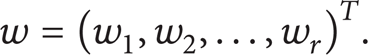
Assume that the input signal sample is x = [x1, x2,…, xm0] T (m0-dimensional vector) and the training sample set is {(x i , d i )}i − 1 N . The nodes in hidden layer is m1. So each input signal mode generates m1-dimensional implicit space vector ϕ(x) = [ϕ1(x), ϕ2(x),…, ϕ m (x)] T consisted of the radial basis functions. Assume that the connection weight between neuron j in the hidden layer and neuron i in the input layer is w ji . Thus the connection weight vector is described as follows:

The connection weight matrix between neurons in the radial basis layer (hidden layer) and neurons in the input layer is described as
The radial basis function in hidden nodes most commonly adopts Gaussian function shown as follows:

where c i is the center vector of neurons and σ i is the width parameter of the kernel function. The linear mapping from the hidden layer to the output layer is described as

where b is the offset of the output neurons. By calculating synaptic weights and thresholds of output units, the RBFNN model is set up.
3.3. Learning Algorithm of RBFNN
The main purpose of the RBFNN learning algorithm is to determine the centre c of each unit, radius σ i , and the mediation weight matrix w. The training procedure is described as follows.
The auxiliary variables are carried out in the scale transformation or normalization in order to remove those samples with larger errors. The periodicity, fixed change trend, or other relationships of the retained samples are analyzed to facilitate the training of RBFNN.
Given the initial vector centre c i (0) = (i = 1, 2,…, q) of the RBFNN hidden nodes, the learning rate β(0) (0 < β(0) < 1) and the threshold ε are used to determine whether the calculation is stopped or not.
Calculate the Euclidean distance and determine the nodes with minimum distance:

where k is the sample number and r is the serial number of the hidden node whose distance between the centre vector c i (k − 1) and the input sample x(k) is nearest.
The K-means clustering algorithm is adopted to adjust the centre vector c i of the nodes in hidden layer:
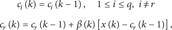
where β(k) is the learning rate, which gradually reduces to zero with the increase of learning samples:
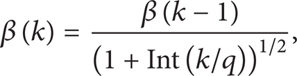
where Int(k/q) represents a rounding operation for k/q.
All samples k (k = 1, 2,…, N) are carried out in the steps (3) and (4) repeatedly until they satisfy the followed criteria:

After determining c i , the connection weights w ki (k = 1, 2,…, L;i = 1, 2,…, q) between the hidden layer and output layer can be calculated based on the following equation:
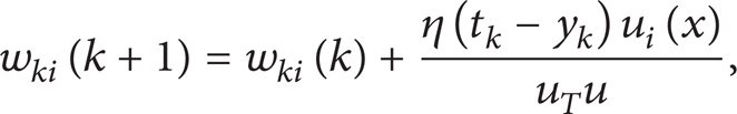
where u = [u1(x), u2(x),…, u q (x)] T , u i (x) is Gaussian function, and η is the learning rate.
4. RBFNN Soft-Sensor Model Optimized by Improved AFSA
4.1. Artificial Fish Swarm Algorithm
With the development of the swarm intelligent algorithms, the evolutionary algorithm [16], the genetic algorithm [17], the particle swarm optimization [18], and the differential evolution [19] have been adopted to optimize the structure parameters of RBF neural network. Artificial fish swarm algorithm (AFSA) is an intelligent optimization algorithm simulating fish swarm behavior, such as foraging, swarming, chasing, random, in the search domain for optimization [20–22]. In the fish swarm pattern, the method described in Figure 4 is adopted to simulate the visual sensor system of the artificial fish. Suppose that X is the current location of the artificial fish entity, Xn1 and Xn2 are position of two fish within visual sight, and X v is viewpoint position in certain time. If the food consistency of X v is higher than the food consistency of X, the artificial fish moves one step toward the X v direction to reach location Xnext, where X = (x1, x2,…, x n ) and X v = (x1 v , x2 v ,…, x n v ) in Figure 4. Otherwise keep patrolling within visual field scope. So the learning process can be expressed as follows:
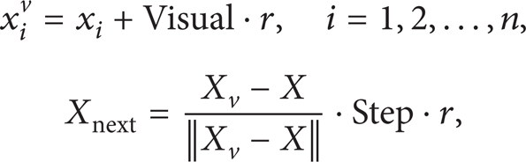
where r is a random number in the scope [− 1, 1].

Visual scope and moving step of artificial fish.
Because the number of the individuals is limited in environment, therefore, the method to percept the associate positions in the view and adjust their own corresponding positions is similar to the above method.
4.2. Realization of Artificial Fish Swarm Algorithm
The fish swarm behaviors of AFSA are initialization, foraging, swarm, and searching behavior [11]. The variable parameters in AFSA algorithm are listed in Table 1.
Variable parameters of AFSA.

(1) Initialization of Fish Swarm. Each artificial fish is a set of random real numbers within given limits. For example, the size of fish swarm is N. There are two parameters x and y to be optimized, whose scope is [x1, x2] and [y1, y2], respectively. Then an initial fish swarm with 2 columns and N rows will be produced, where each column represents an artificial fish with two optimized parameters.
(2) Foraging Behavior. If the current state of the artificial fish is X i and the current cycle of the foraging behavior n = 0, one state X j within Visual is randomly chosen. Then obtain

Because the maximum and minimum problem can be mutual converted, the maximum problem is discussed in the paper. If Y i < Y j , go forward one step to that direction, which is described as follows:

If Y i < Y j , the new X j is selected to be carried out in the above steps. By repeating Try_number times, namely, n ≥ Try_number, if still not reaching the forward moving condition, a forward step is carried out randomly; that is to say,

(3) Swarming Behavior. Suppose that the current state of the artificial fish is X i . In the range of d i,j < Visual, the number of partners is n f , the central position is X c , and δ is the congestion degree. (Y j /n f ) > δY i represents that the food concentration in partner centre is higher than the current state and the congestion degree is not too large, so the artificial fish moves a step forward to the direction to obtain
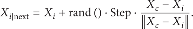
Otherwise, implement the foraging behavior.
(4) Following Behavior. Suppose that the current state of the artificial fish current state is X i , the number of the artificial fish partners within the scope of view (d i,j < Visual) is n f , and the Y j in the partners is the largest partner X j . (Y j /n f ) > δY i represents that the food concentration near state X j is relatively high and the congestion degree is not too large, so the artificial fish moves a step forward to the direction of partner X j to obtain

Otherwise, implement the foraging behavior.
4.3. Algorithm Procedure
The algorithm procedure of the mutation operator based AFSA for optimizing the RBFNN soft-sensor model is described as follows.
Initialize the parameters of RBFNN: the initial vectors center c i (0) = (i = 1, 2,…, q), learning rate β(0), and threshold ε. Initialize the parameters of AFSA: the number of initial artificial fish N, vision scope Visual, step length step, and the crowding factor δ(delta). Record the initial state X i = (x1, x2,…, x n ) of the artificial fish in the bulletin board. Initialize the number of initial iterations GenNum = 0, the number of maximum iterations MaxGen, and the maximum attempt number of the foraging behavior Try_number.
The sample data of melting speed and polar cone purification coefficient of consumable electrodes are divided into training samples and testing samples. The training samples are preprocessed by normalization and fed into the RBFNN soft-sensor model. After antinormalization processing, the predictive results are compared with the actual values to obtain the prediction error error i (i = 1, 2,…, n).
The artificial fish swarm algorithm firstly carries out the cluster analysis for the received error results and distributes an artificial fish swarm including N artificial fish in every cluster class. According to each type of error data, each artificial fish swarm is optimized, and the state of the optimal artificial fish is recorded in the bulletin board every time.
According the optimized results of the AFSA, the proposed algorithm is used to adjust the vector center c i (0)(i = 1, 2,…, q) of all nodes in the hidden layer and the learning rate β(0) and promptly revise the connection weights w ki between the hidden layer and the output layer.
Judge termination condition. If the maximum iteration number MaxGen is reached, the optimum results are outputted, namely, the bulletin board value. Otherwise, GenNum = GenNum + 1 and go back to the step (3).
5. Simulation Results
This paper adopts the production data matrix of six process variables (the remelting current, the remelting voltage, slag pool depth, cooling water flow, outlet water temperature of the cooling water, and the cone head height of consumable electrodes) collected in the ESR industrial field to establish two soft-sensor models based on RBFNN for predicting the melting rate and the cone purifying coefficients of consumable electrodes, respectively. Then AFSA is adopted to optimize the model structures parameters of RBFNN, which includes the centers and widths of base functions in the hidden layers and the network connectivity weights. The structure of the RBFNN is 6-25-1 and the number of hidden layer nodes is 25, which is mainly decided according to experiences. So the number of the total optimized parameters is 75. Because the input and output variables of the soft-sensor model are normalized to [− 1, 1], so the search range of the final optimized parameter is located in the scope [− 1, 1]. The initialization parameters of AFSA are as follow: artificial fish swarm size N = 100, perceived distance Visual = 1, mobile step Step = 0.5, the number of maximum iterations is 50, and the number of the foraging maximum tentative is 100.
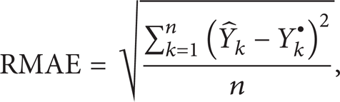
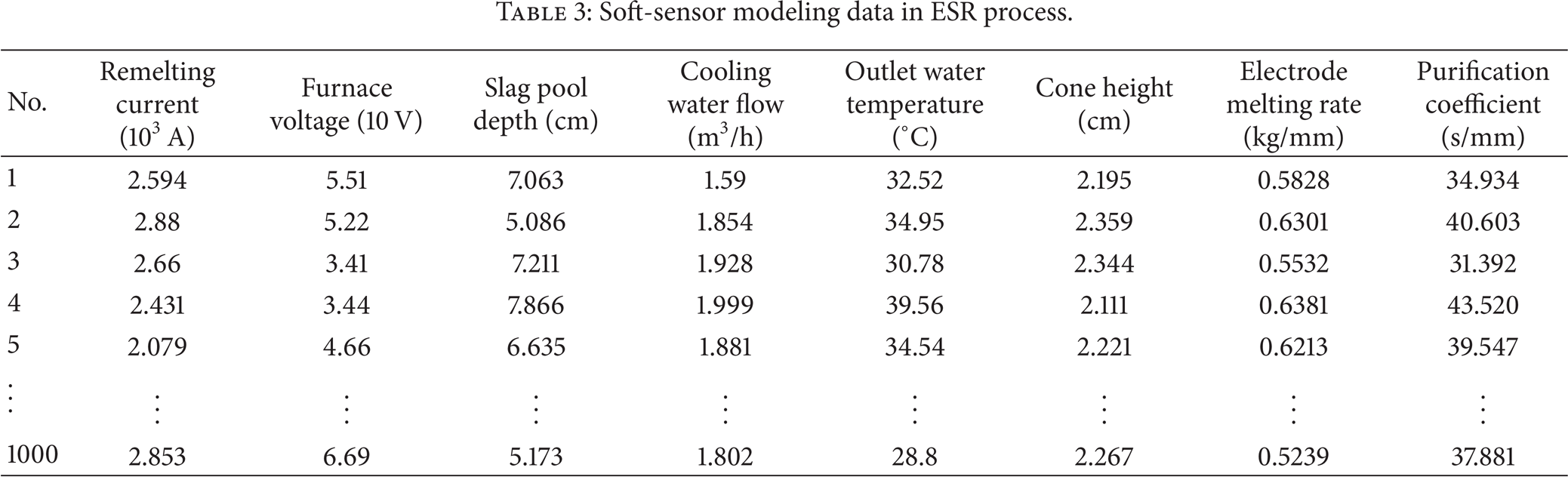
Before soft-sensor modeling of ESR process, for the sake of weighing the predictive performance of the proposed model, four performance index functions, such as maximum positive error (MPE), maximum negative error (MNE), root mean square error (RMSE), and sum of square error (SSE), are defined in Table 2, where ŷ is the predictive value and y is actual value. 1000 uniform and representative historical data of ESR process are chosen as the experiment data shown in Table 3. After the data pretreatment, the former 900 sets of datum are selected as the training data to be used to train the RBFNN. The other datum is used to verify the performance of the soft-sensor model.
Performance index functions.

Soft-sensor modeling data in ESR process.
Firstly, three kinds of learning algorithms of RBFNN, such as gradient method, clustering method and orthogonal least square (OLS) method, and the MLP neural network, are used to set up the soft-sensor models, respectively, in order to predict the melting rate and the cone purifying coefficients of consumable electrodes of ESR process. The predictive output and actual output under three methods are shown in Figure 5. The predictive error curves are shown in Figure 6. Seen from prediction output curves and prediction error curves, it can be seen that the OLS-based RBFNN has better prediction effect than the other methods. Therefore, the OLS-based RBFNN soft-sensor model is adopted to be compared with the other swarm intelligent based RBFNN soft-sensor model.

Predicted output curves.

Predicted error curves.
In order to highlight the superiority of the proposed method, the comparisons have been made among OLS-based RBFNN soft-sensor model, the GA based RBFNN soft-sensor model (GA-RBFNN), and the PSO based RBFNN soft-sensor model (PSO-RBFNN). The predictive outputs under four methods are shown in Figures 7 and 8.
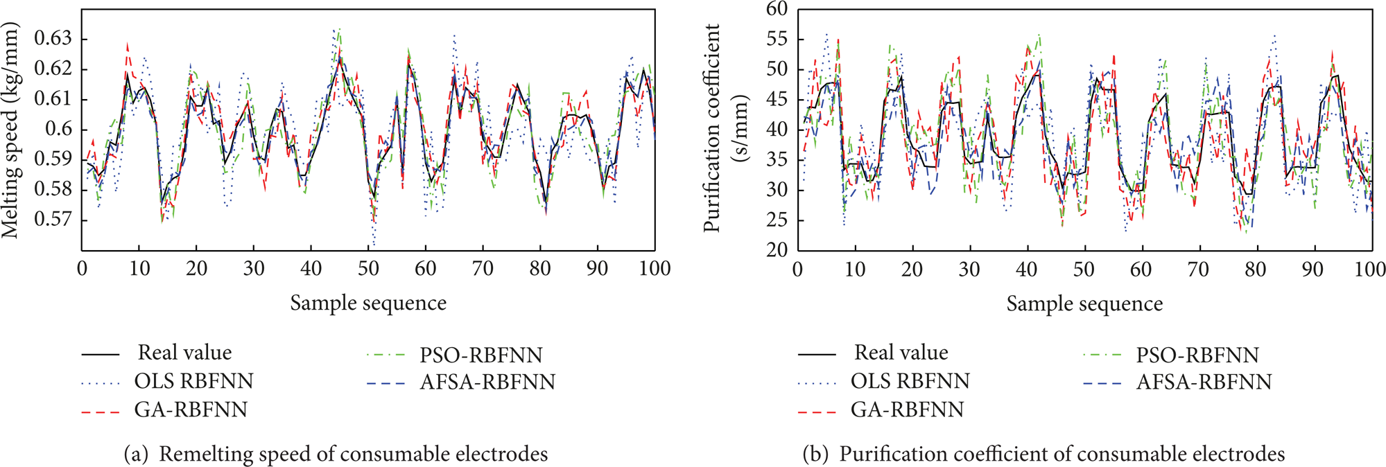
Predicted output curves.
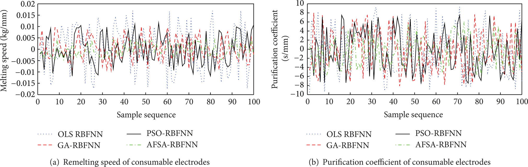
Predicted error curves.
The predictive simulation has been carried out 10 times. Then the statistics analysis results of the model performances with 10 runs are listed in Table 4 based on the definition of predictive performance index in Table 2. Performance comparisons in the computational time are listed in Table 5. Seen from the simulation results, the proposed AFSA-RBFNN predictive model has higher accuracy than the MLP neural network, GA-RBFNN, and PSO-RBFNN soft-sensor model. The successful adoption of the predictive model in the ESR process for obtaining the real-time remelting speed and purification coefficient of consumable electrodes has important significance in the field of improving the production capacity and reducing production costs.
Comparison of performance index under different predictive models.

Performance comparisons in computational time for training different predictive models.

Simulation results show that the AFSA-RBFNN soft-sensor model proposed in this paper has strong approximation ability and the prediction accuracy of melting speed and purification coefficient of consumable electrodes in ESR process. Optimization control of the ESR process based on the prediction model will surely have a great significance on system stability.
6. Conclusion
Based on the good nonlinear approximation capability of RBFNN, the simple and easy realization, the capability of global optimization and avoidness of trapping into local optimum, and the durativity to the searching space and other distinguishing features of the artificial fish swarm algorithm, the paper puts forward an AFSA-RBFNN model to predict the melting rate and cone purification coefficient of the consumable electrode in the ESR process. The simulation results show that the proposed method has a good tracking rate and a high estimation accuracy and can realize predictive control of a technical index. Furthermore, it fully satisfies the real-time control requirements of ESR process.
Conflict of Interests
The authors declare that there is no conflict of interests regarding the publication of this article.
Footnotes
Acknowledgments
This work is partially supported by the Program for China Postdoctoral Science Foundation (Grant no. 20110491510), the Program for Liaoning Excellent Talents in University (Grant no. LJQ2011027), the Program for Anshan Science and Technology Project (Grant no. 2011MS11), and the Program for Research Special Foundation of University of Science and Technology of Liaoning (Grant no. 2011zx10).