Sage Journals: Discover world-class research

Abstract

The fruit fly optimization algorithm (FOA) is one of the latest nature-inspired computational models. It has the advantages of having a simple mechanism, fewer control variables, and a fast convergence. However, most applications of the FOA focus on optimization problems in a continuous space. Three-dimensional path planning is a typical discrete optimization problem and can be attributed to multivariable and multiobjective optimization computations. In this paper, we advance an improved FOA model (IFOA) based on engineering techniques. This model is then used to solve for the three-dimensional (3D) path planning of a robot. In a simulation experiment conducted in a virtual three-dimensional space, the IFOA was shown to have a certain capability for three-dimensional path planning. Although the accuracy of the IFOA seems slightly weaker than that of ant colony optimization (ACO), the IFOA may confer time savings of 25% and has greater efficiency. Therefore, this new model still provides a novel and valuable means for solving such discrete optimization problems.

1. Introduction

Generally, the three-dimensional path planning of robot can be defined simply in a given three-dimensional map. It is used to find the shortest path from the starting point to the target location [1, 2]. In the process of stepping forward to the destination, the robots need to avoid obstacles within the three-dimensional space and any locations that are difficult to cross. For example, the general underwater robot can move forward and backward, left and right, and up; however, it cannot jump, as it is hard to climb a very steep slope. Currently, the mature path planning of robots is still in the one-dimensional and two-dimensional field stages.

In three dimensions, the path planning of robot is challenging given the computing complexity, the large required information storage with multivariable and multiobjective constraints, and the difficulty in searching directly for the global optimization path. In engineering applications, three-dimensional path planning has been widely used in devices including mining robots, lunar rovers, EOD robots, underwater robots, and space detectors. Currently, the representative research on the problems of 3D path planning has achieved the following solutions: the A^* algorithm, integer programming, the genetic algorithm, the particle swarm algorithm, and the ant colony algorithm [2 –6]. However, in searching for the optimal path, the computation of the A^* algorithm would be more difficult with an added dimension. The integer programming method attempts to simply transform the 2D path planning framework onto a three-dimensional domain. Given the strict constraint conditions, it is not easy to meet the needs of real environments. The genetic algorithm and particle swarm algorithm have been applied to path planning but have also encountered similar problems. Some scholars have even argued that most research on path planning of robots based on GA and PSO is not completely 3D path planning [7]. Typically, by considering the constraints of the assumed rules, solving the problem of path optimization in a three-dimensional space may utilize sampling, segmentation, rotation, and other methods to discretize the three-dimensional space. Through the discretization of a continuous space, 3D space can be transformed into an observable point set. Due to the capability of concurrent computing and the advantages of rapid convergence, the ant colony algorithm and its improved models have been applied to path planning for an underwater robot [7]. Some related research on path planning in 3D space has reported that the ant colony algorithm and its improved models seem to have a better performance. Compared with other swarm intelligence models, the ACO seems to be more effective for the 3D path planning of a robot [7, 8].

2. How to Transform a Three-Dimensional Space into a Discrete Point Set for Path Planning

To transform a continuous pace into a discrete point set, we can generally construct a cuboid to cover the search area of the robot [4, 8]. For example, assuming the robot is assigned to search a given area of the ocean floor (20 km (length) * 20 km (width) * 1 km (height)) then we can construct a cuboid (21 km * 21 km * 1 km) to wholly cover the assigned ocean floor in three dimensions. Suppose the three-dimensional cuboid can be, respectively, aliquoted into n, m, and l parts in the x-axis, y-axis, and z-axis. In this case, the points in the three-dimensional space can be made into discrete sets of points on two coordinates (Figure 1). Each point has an ordinal coordinate Coordinate_order and position coordinate Coordinate_location, which are shown in

\begin{matrix} Point (C o o r d i n a t e_o r d e r) = {(i, j, k) ∣ i \in [0, n]; j \in [0, m]; k \in [0, k]}, n, m, k > 0, \\ Point (C o o r d i n a t e_l o c a t i o n) = {(x_{i}, y_{j}, z_{k}) ∣ i \in [0, n]; j \in [0, m]; k \in [0, k]}, n, m, k > 0 . \end{matrix}

(1)

Figure 1:

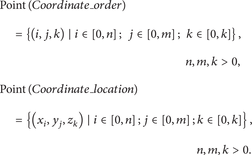
Segment of three-dimensional space in robot path planning.

For ease of calculation, in the following simulation experiments, the serial number coordinates are adopted first. When we need to calculate the distance between two points, the location coordinates are used.

3. The Fruit Fly Optimization Algorithm and Strategies for Improvement

The olfactory organ of the fruit fly can commendably collect all types of floating scents in the air. It can even smell food up to 40 KM away. The fruit fly optimization algorithm (FOA) is a novel global optimization computational method based on the foraging behavior of fruit flies. It was proposed by Pan [9, 10].

3.1. Basic Concepts and Computing Steps of FOA

Inspired by the food searching behaviors of the fruit fly group, FOA is divided into several basic steps [9].

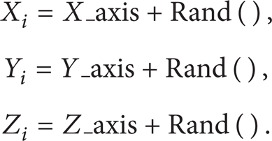
Step 1. Randomized initial fruit fly swarm location matrix:

Init X_axis; Init Y_axis; Init Z_axis .

(2)

Step 2. Each fruit fly group is assigned a random direction and distance for the food search:

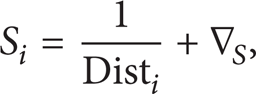
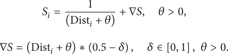
\begin{matrix} X_{i} = X_axis + Rand (), \\ Y_{i} = Y_axis + Rand (), \\ Z_{i} = Z_axis + Rand () . \end{matrix}

(3)

Step 3. As the food location cannot be known, the distance to the origin is thus estimated first (Dist). Then, the smell concentration judgment value (S) is calculated. This value is the reciprocal of the distance. To solve the problem that value of a smell cannot be negative, some scholars have argued that a modifying factor ∇_S should be added to the smell function. In this way, the FOA could have wider range of applications for global optimization [11]. Consider

{Dist}_{i} = \sqrt{X_{i} + Y_{i} + Z_{i}},

(4)

S_{i} = \frac{1}{{Dist}_{i}} + \nabla_{S},

(5)

\nabla_{S} = {Dist}_{i} * (0.5 - δ), δ \in [0, 1] .

(6)

Step 4. Substitute the smell concentration judgment value (S) into the fitness function, to determine the smell concentration (Smell_i) of the individual location of the fruit fly:

Smel l_{i} = f_{fitness} (S_{i}) .

(7)

Step 5. Identify the fruit fly with the maximal smell concentration (finding the maximal value or the minimum value) among the fruit fly swarm:

Get [bestSmell bestIndex] = \max (Smell) .

(8)

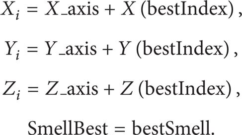
Step 6. Keep the best smell concentration value (fitness) and the coordinates (X,Y,Z). The fruit fly swarm will then use vision to fly towards that location:

\begin{matrix} X_{i} = X_axis + X (bestIndex), \\ Y_{i} = Y_axis + Y (bestIndex), \\ Z_{i} = Z_axis + Z (bestIndex), \\ SmellBest = bestSmell . \end{matrix}

(9)

Step 7. Repeat the implementation of Steps 2–5; then judge if the smell concentration is higher than the previous iterative smell concentration. If so, implement Step 6.

3.2. Improvement Strategies for the FOA

Since FOA has been proposed, its applications have emerged gradually. In the past several years, scholars have attempted to apply FOA to such fields as PID parameter controller optimization, the prediction of an electric power load, and the knapsack problem [12 –16]. The fruit fly optimization algorithm has certain global optimization capabilities but can also achieve fast convergence in combination with other models, to promote computational efficiency by narrowing down the scope of the optimization space. However, the basic FOA and some modified versions can easily fall into the local optimum in global optimization computations, and the stability of the algorithm must be further promoted [8, 9]. First, because the variable of smell is the inverse of distance, which can be equal to zero when the coordinates of two points are the same, computing the smell will encounter a bug in running the code. In addition, ((6)) is modified to allow the value of the smell concentration (fitness) to be negative [11], but it is functional only when the value of distance D is bigger than 1. Therefore, the modified FOA still has some limitations. To overcome the shortcomings of the MFOA, the basic FOA needs to be modified further, and the modified results are shown in

\begin{matrix} S_{i} = \frac{1}{(Dis t_{i} + θ)} + \nabla S, θ > 0, \\ \nabla S = ({Dist}_{i} + θ) * (0.5 - δ), δ \in [0, 1], θ > 0 . \end{matrix}

(10)

In ((10)), a revision parameter θ is added, the value of which is always positive. In the real applications of FOA, the parameter θ can be adjusted to be fit for the computation tasks. When choosing the next point, the decision-making rule of FOA is based only on the mechanism of random movement and the distance between the current point and the original point in the coordinate system. Obviously, it is difficult to solve the discrete optimization problem using the traditional FOA. In the latest research related to FOA and its applications, very few articles have considered global optimization in discrete space. Therefore, the strategy of whole random movement should be improved to meet the needs of discrete optimization problems. The decision-making strategies of “choose the next point” or “choose the next position” should be put into the basic FOA. Here, a composite distance is introduced to improve the movement tactics of the fruit fly. The composite distance Dist_i is designed to be a linear function related to three distances: (1) between the current point and the next point, (2) between the next point and the target point (if the target point is known), and (3) between the current point and the original point. This is shown in

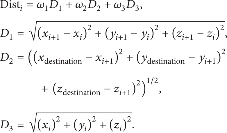
Dis t_{i} = ω_{1} D_{1} + ω_{2} D_{2} + ω_{3} D_{3}, D_{1} = \sqrt{{(x_{i + 1} - x_{i})}^{2} + {(y_{i + 1} - y_{i})}^{2} + {(z_{i + 1} - z_{i})}^{2}}, D_{2} = ({(x_{destination} - x_{i + 1})}^{2} + {(y_{destination} - y_{i + 1})}^{2} {+ {(z_{destination} - z_{i + 1})}^{2})}^{1 / 2}, D_{3} = \sqrt{{(x_{i})}^{2} + {(y_{i})}^{2} + {(z_{i})}^{2}} .

(11)

Of course, ((4)) is not the perfect solution. For example, if the target point is not known and the weight of D₂ is equal to zero, then the composite distance will lose some important information. However, ((4)) can expand the application range from continuous space to discrete space. In fact, when the weights ω2 and ω3 are assigned values of zero, then the improved FOA can return to the naïve FOA.

4. Visual Neighborhood Constraints of a Robot in Search Space

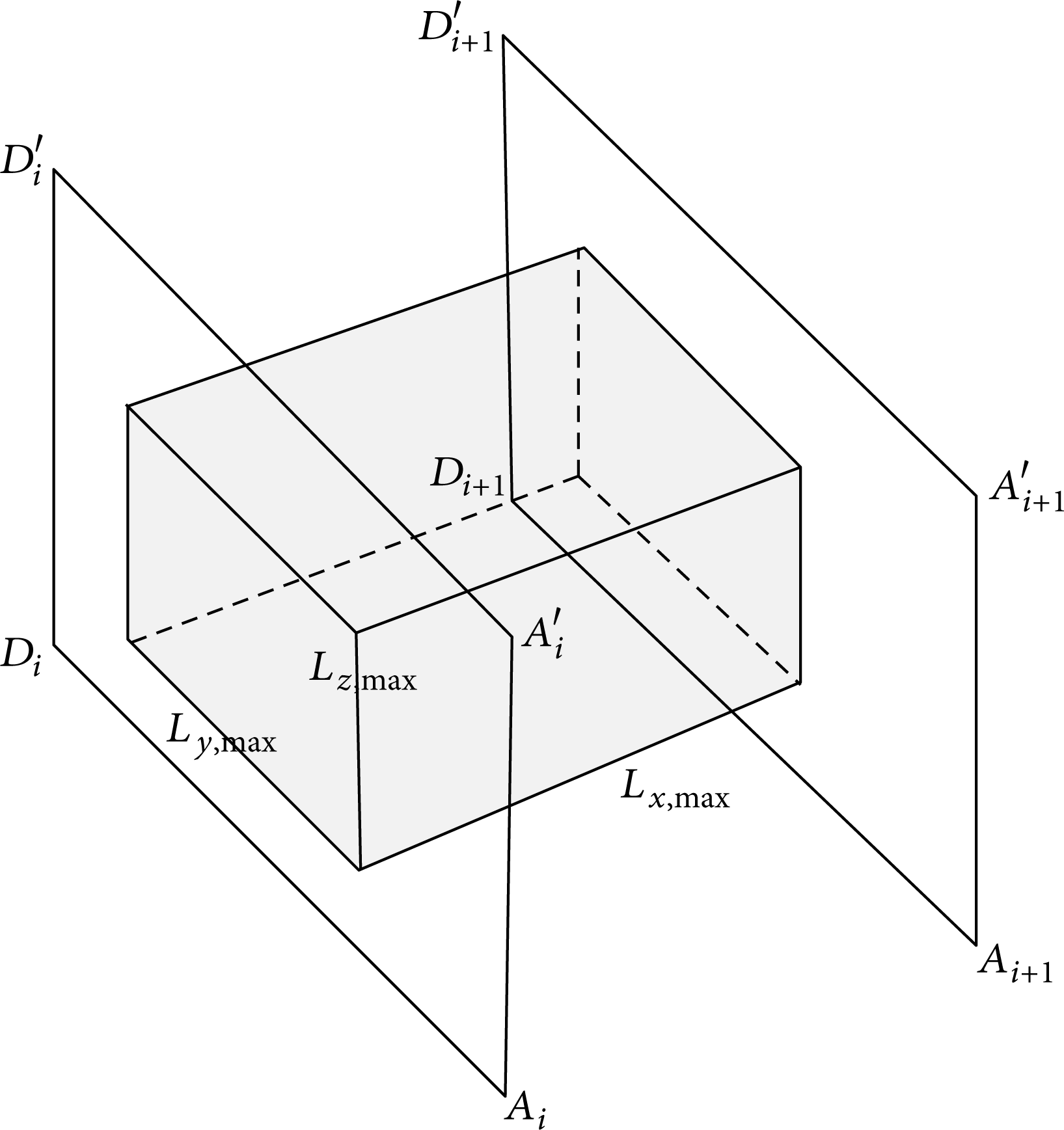
In general, the movement of a robot can be divided into forward, horizontal, and upwards, corresponding to the x-axis, y-axis, and z-axis of a three-dimensional coordinate system. To simplify the problem, suppose the x-axis is the forward direction. Considering that an underwater robot has a visual field constraint, the maximum observable and movable distance of the three axes can be assumed. Therefore, when the robot is located in a certain position, it can only hunt for the next node within the scope of its limited space. This behavior simplifies the search space and increases its efficiency to some extent [7]. A schematic diagram of this visual constraint is shown in Figure 2.

Figure 2:

Neighboring visual space of a fruit fly.

In Figure 2, the visual neighborhood constraint narrows down the search space for each of fruit fly group when they need to choose the next point. This constraint is necessary for the robot. For example, the popular AUV (autonomous underwater vehicle) adopted the pedrail system or propulsion system, as the directions and range of robot action have limitations.

According to the visual scope constraint shown in Figure 2, when the fruit flies move to the next point, the neighbor space of choice is shown, given by

P_{neighbor} = {(x, y, z) ∣ x \in [- L_{x, \max}, L_{x, \max}]; y \in [- L_{y, \max}, L_{y, \max}]; y \in [- L_{z, \max}, L_{z, \max}]} .

(12)

To simplify the computation of the 3D path planning, we assume that the fruit fly steps forward with a fixed length in the direction of a single axis. Then, the next point set can be written as

number of next choices = L_{y, \max} * L_{z, \max} .

(13)

From ((13)), the length of the step in the x-axis, y-axis, and z-axis directions may influence the computational complexity of the FOA. Compared to ((13)), the computing time cost will increase when adopting the whole random movement in three directions. In addition to this, the set size of the visual next points can affect the efficiency of the FOA. These are the common challenges in the 3D path planning of a robot.

5. Improving FOA and Its Simulations in Three-Dimensional Path Planning

5.1. Improvement and Simulation of the FOA Algorithm

FOA is the latest swarm intelligence algorithm. Its advantages include fewer control parameters, lower computational complexity, and the ability for global optimization. Although the FOA has been partially confirmed in extreme optimization and predictive areas, there are some obvious defects. For example, although the FOA has fewer control parameters, it can oscillate when there are multiple local extreme values [11]. Compared to the ant colony algorithm, the FOA has simpler parameters and control variables and lower computational complexity; however, it also lacks the positive feedback mechanism of the ant colony algorithm. The positive feedback mechanism of the ant colony algorithm has been proven to have fast convergence and to improve the efficiency in solving discrete space optimization problems. As a novel nature-inspired algorithm, there are still very few research articles describing solving discrete optimization problems using the FOA. From the biological point of view, fruit flies have better visual systems than ants; thus, they have obstacle avoidance and spatial navigation abilities based on their vision and olfactory sensations. Therefore, they do not need pheromone secretion to strengthen their paths. Thus, the addition of a visual feedback mechanism to the traditional FOA is considered here. Fruit flies have a certain visual ability and can effectively distinguish an unreachable neighboring point. When choosing their next point, they will be influenced by the visible distance between that point and their own position. They will also take into account the food concentration at that point. Therefore, the probability of fruit flies selecting the next point p(next) is

p (next) = {\begin{cases} \frac{ω_{1} Visual (j) + ω_{2} S (j)}{\sum (ω_{1} Visual (j) + ω_{2} S (j))}, \\ j \in {reachable neighbors}, \\ 0, j \in {unreachable neighbors} . \end{cases}

(14)

In ((14)), S(j) provides information about the food concentration of the visual reachable point j of the fruit fly, while Visual (j) is the reciprocal of the distance between point j and the position of the fruit fly. ω₁ and ω₂ are weights, and ω₁ + ω₂ = 1.

To compare the FOA to the ant colony algorithm, we have chosen a virtual underwater environment from [7] and have used their start and end points for the simulating calculation. A simulation of the underwater environment is shown in Figure 5, and the 3D space of route planning is defined as 20 Km(x) * 20 Km(y) * 2000 m (height). Here, the distance between each node of the x-axis and y-axis is one kilometer, while the node spacing in the z-axis is 200 meters. In Figure 3, the starting point coordinate is Start (1, 10, 4) and the target point is End (21, 4, 5).

Figure 3:

The route planning space.

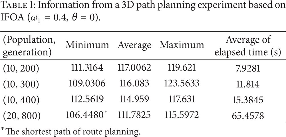
Because the distances in this computation are all bigger than 1, the revision parameter θ can be assigned to zero and ω₁ to 0.4 in the simulation experiments. The initial population is 10 and 20, and the iteration times are set at 200, 300, 400, and 800. The simulation tool used was MATLAB7.0, and the hardware environment was core i5, 2.53 GHz, and 2 G memory. The results of this simulation are shown in Table 1 and Figures 4 and 5.

Table 1:

Information from a 3D path planning experiment based on IFOA (ω₁ = 0.4, θ = 0).

(Population, generation)	Minimum	Average	Maximum	Average of elapsed time (s)

(10, 200)	111.3164	117.0062	119.621	7.9281
(10, 300)	109.0306	116.083	123.5633	11.814
(10, 400)	112.5619	114.959	117.631	15.3845
(20, 800)	106.4480^*	111.7825	115.5972	65.4578

$^{*}$ The shortest path of route planning.

Figure 4:

The best result of route planning based on IFOA with the parameters P = 20, G = 800, and ω₁ = 0.4.

Figure 5:

The best fitness evolution based on IFOA with the parameters P = 20, G = 800, and ω₁ = 0.4.

To test the influence of weight ω₁ on the efficiency and accuracy of the FOA, the second simulation experiment used ω₁ = 0.7, a fruit fly population of 5, 10, and 20, and iteration times (generations) of 200, 300, and 400. The results of this experiment are shown in Table 2 and in Figures 6, 7, 8, 9, 10, and 11.

Table 2:

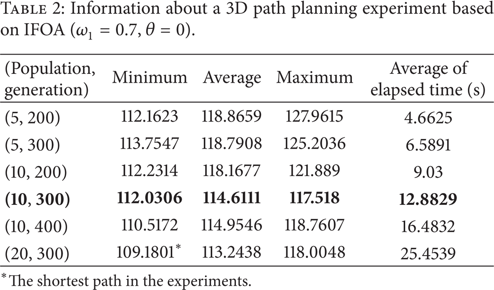
Information about a 3D path planning experiment based on IFOA (ω₁ = 0.7, θ = 0).

(Population, generation)	Minimum	Average	Maximum	Average of elapsed time (s)

(5, 200)	112.1623	118.8659	127.9615	4.6625
(5, 300)	113.7547	118.7908	125.2036	6.5891
(10, 200)	112.2314	118.1677	121.889	9.03
(10, 300)	112.0306	114.6111	117.518	12.8829
(10, 400)	110.5172	114.9546	118.7607	16.4832
(20, 300)	109.1801^*	113.2438	118.0048	25.4539

$^{*}$ The shortest path in the experiments.

Figure 6:

(a) One of the best results with the combination (P = 5, G = 200, and ω₁ = 0.7). (b) One of the shortest paths with the combination (P = 5, G = 200, and ω₁ = 0.7).

Figure 7:

(a) One of the best results with the combination (P = 5, G = 300, and ω₁ = 0.7). (b) One of the shortest paths with the combination (P = 5, G = 300, and ω₁ = 0.7).

Figure 8:

(a) One of the best results with the combination (P = 10, G = 200, and ω₁ = 0.7). (b) One of the shortest paths with the combination (P = 10, G = 200, and ω₁ = 0.7).

Figure 9:

(a) One of the best results with the combination (P = 10, G = 300, and ω₁ = 0.7). (b) One of the shortest paths with the combination (P = 10, G = 300, and ω₁ = 0.7).

Figure 10:

(a) One of the best results with the combination (P = 10, G = 400, and ω₁ = 0.7). (b) One of the shortest paths with the combination (P = 10, G = 400, and ω₁ = 0.7).

Figure 11:

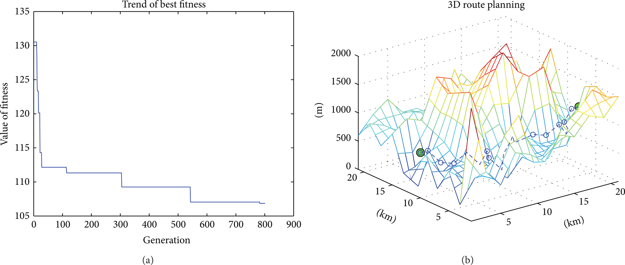
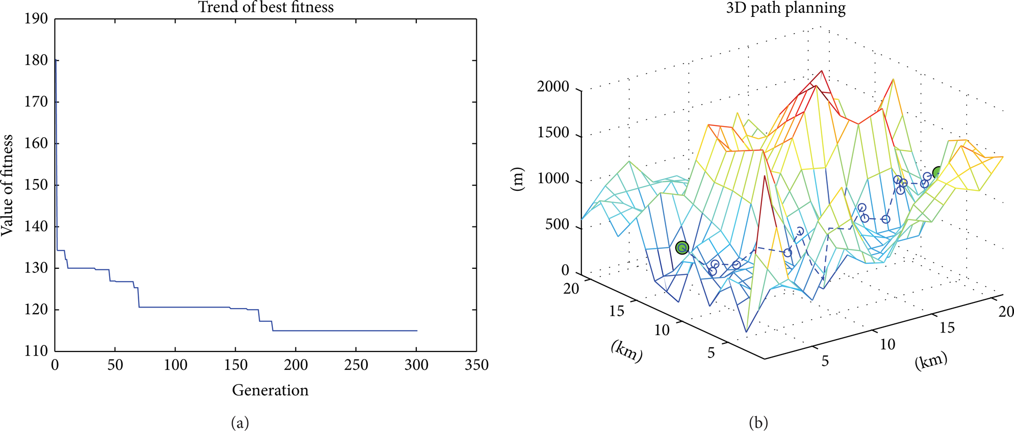
(a) One of the best results with the combination (P = 20, G = 300, and ω₁ = 0.7). (b) One of the shortest paths with the combination (P = 20, G = 300, and ω₁ = 0.7).

From the results of the comparison experiments, we can argue that the weight ω₁ can slightly affect the accuracy and efficiency of the IFOA. When we enhance the weight of the distance between the current point and the next point, we slightly decrease the accuracy and efficiency. It is thus reasonable that the distance between the next point and the food source seems more important in IFOA. Through repeated experiments, we chose a preferable value combination of parameters for the IFOA: population = 10, generation = 300, and ω₁ = 0.4. This combination of parameters was then adopted for the following experiments assessing the ant colony optimization algorithm in the three-dimensional path planning of robot.

5.2. Comparison Experiments among FOA, IFOA, and ACO in 3D Path Planning

Typical applications of 3D path planning using swarm intelligence are based on the ant colony algorithm. Therefore, to analyze the performance of the naïve FOA and IFOA in three-dimensional path planning, the ant colony optimization (ACO) was chosen as the algorithm for comparison [7, 17]. The population of the ant colony was set at 10 and 20, and iteration times were set at 200, 200, 400, and 800. The start point and end point are the same with the IFOA. The results of this experiment are shown in Table 3 and Figure 12.

Table 3:

Simulation of 3D path planning based on the ant colony algorithm (α = β = 0.5, ρ = 0.2).

(Population, generation)	Minimum	Average	Maximum	Average of elapsed time (s)

(10, 200)	112.9615	115.0194	118.4994	10.5423
(10, 300)	107.8204	114.1272	119.0625	14.6312
(10, 400)	107.5266	110.7758	114.3725	18.4562
(20, 800)	106.952^*	108.8688	110.4913	77.3202

$^{*}$ The shortest path of the experiments based on ACO.

Figure 12:

(a) One of best results of route planning based on ACO with (P = 20, G = 800, α = β = 0.5, and ρ = 0.2). (b) One of the shortest paths based on ACO with (P = 20, G = 800, α = β = 0.5, and ρ = 0.2).

5.3. Analysis of the Simulation Results

Because there is little research on the use of the FOA in discrete optimization, we chose a basic ant colony algorithm as the reference for our control experiments, as this is one of the best intelligent computing models available for discrete global optimization. The detailed results of a comparison based on our simulation experiments are shown in Table 4.

Table 4:

Comparison details between ACO and IFOA, FOA (population = 10, generations ∈ (200, 300, 400)).

Generations	BestFitness			Elapsed time (s)
Generations	ACO	IFOA	FOA	ACO	IFOA	FOA

200	115.0579	118.9934	159.331	10.016	8.015	7.633
	116.1623	117.2939	188.3901	10.797	8.125	8.012
	112.9615	111.3164	219.353	10.828	7.922	8.644
	115.1509	116.8909	190.4533	9.688	8.39	8.012
	114.8476	119.621	153.356	10.453	7.625	7.121
	114.1703	117.3258	177.3352	11.484	7.422	6.931
	114.0146	117.6663	201.112	10.985	7.766	7.781
	115.1784	115.395	199.322	10.672	7.469	7.113
	118.4994	119.0978	142.433	9.828	7.719	7.093
	114.1509	116.462	149.355	10.672	8.828	7.391

300	107.8204	109.0306	179.123	15.813	12.328	12.011
	115.0545	114.7673	163.3577	13.953	11.828	10.923
	114.302	114.3677	159.2391	14	12.437	11.935
	116.2326	112.6629	149.3312	14.766	10.859	11.035
	113.4064	113.119	139.3091	14.703	10.844	9.799
	115.9262	123.0659	183.2321	14.437	12.515	10.385
	110.3358	118.0851	192.335	14.625	10.657	12.312
	119.0625	123.5633	205.7791	14.172	11.875	12.032
	115.4302	117.8671	177.3231	14.89	12.828	12.344
	114.7016	114.302	153.9632	14.953	11.969	11.399

400	109.1881	116.4847	169.8821	19.172	14.953	13.595
	109.7965	114.3244	193.0921	18.75	14.594	14.053
	112.0932	113.6276	187.351	19.641	14.75	15.091
	107.5266	114.8557	159.0122	18.656	15.782	16.073
	111.127	116.3631	144.773	19.875	14.25	14.87
	110.395	115.5266	169.321	19.25	15.5	14.732
	114.3725	114.1236	139.351	16.687	16.032	15.319
	113.1976	112.5619	188.9013	17.266	16.234	15.977
	112.1976	117.631	195.3351	16.953	15.984	16.013
	107.8637	114.0917	187.3911	18.312	15.766	15.092

From Table 4, we can find that the results of the naïve FOA (basic FOA) are much worse than IFOA and ACO; therefore, we just need to compare IFOA with ACO. According to the detailed experimental data above, “BestFitness” and “generations” are chosen as factors for variance analysis (α = 0.001, tool: spss17.0), and result is shown in Tables 5, 6, 7, and 8.

Table 5:

Test of normality (factor: models).

BestFitness	Kolmogorov-Smirnov^a			Shapiro-Wilk
BestFitness	Statistic	df	Sig.	Statistic	df	Sig.

ACO	.156	30	.060	.948	30	.152
IFOA	.087	30	.200^*	.971	30	.573

$^{a}$ Lilliefors modified significant level.

^*This is the lower limit of the true significance level.

Table 6:

Test of the homogeneity of the variances.

Levene statistic	df1	df2	Sig.

.007	1	58	.935

Table 7:

Test of normality (factor: generations).

Generations	Kolmogorov-Smirnov^a			Shapiro-Wilk
Generations	Statistic	df	Sig.	Statistic	df	Sig.

200	.111	20	.200^*	.975	20	.858
300	.143	20	.200^*	.949	20	.355
400	.116	20	.200^*	.967	20	.699

$^{a}$ Lilliefors modified significance level.

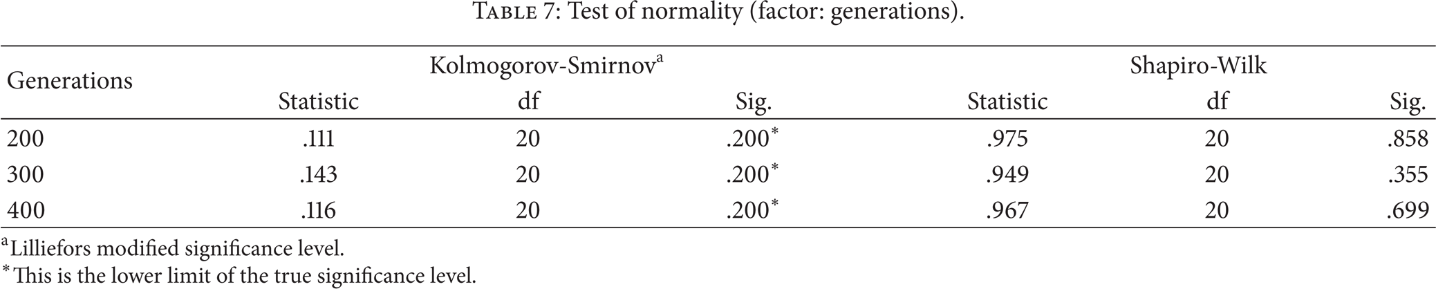
^*This is the lower limit of the true significance level.

Table 8:

Test of the homogeneity of variances.

Levene statistic	df1	df2	Sig.

1.356	2	57	.266

From Tables 5, 6, 7, and 8, both the D-test and the W-test show that the given experimental data obey a normal distribution. Using the test of the homogeneity of variance, we can complete an analysis of the variance (Table 10). The significant test result of the interaction of the double factors is shown in Table 9.

Table 9:

Test of interaction effects among factors.

Source	Type III sum of squares	df	Mean of squares	F	Sig.

Correction model	230.211	5	46.042	5.959	.000
Intercept	789068.928	1	789068.928	102121.852	.000
BestFitness	107.361	1	107.361	13.895	.000
Generation	105.753	2	52.877	6.843	.002
BestFitness * generation	17.097	2	8.548	1.106	.338
Deviation	417.244	54	7.727

Total	789716.383	60
Total of correction	647.455	59

Table 10:

One-way analysis of variance (factor: models) (α = 0.001).

Model	Samples	SUM	Average

BestFitness of ACO	30	3400.2238	113.3407933	8.858471476
BestFitness of IFOA	30	3480.4837	116.0161233	9.765450195

	SS	df	MS	F	P value	F_crit

Between groups	107.3608591	1	107.3608591	11.52935037	0.00124196	4.006872822
Within groups	540.0937285	58	9.311960835

Total	647.4545876	59

Analysis of the interactive factors shows that iteration times do not have an obvious influence on the experimental results, illustrating that the two algorithms have a premature convergence problem in the simulation environment. Although both the ACO and the IFOA can eventually find the shortest path in the virtual environment, the ACO seems slightly more accurate and stable (improved variance). Only from the optimization example of the route planning simulation, the gap in the optimization accuracy between two algorithms is not very obvious. Based on the univariate analysis, the zero hypothesis cannot be rejected in a significance level of α = 0.001. This result is beyond expectations.

5.4. Explanation of the Experimental Results

Compared with ACO, the IFOA is a novel nature-inspired computation model. IFOA has the advantages of having a simple mechanism and fewer control variables. Therefore, IFOA has a faster convergence than ACO. The time complexity of IFOA is computed in Table 11.

Table 11:

Time complexity analysis of IFOA algorithm.

Step	Description	Complexity of runtime

Step 1	Initialize the locations of fruit flies	O(m)
Step 2	Initialize the search direction and stride length for each fly	O(m)
Step 3	Calculate the smell concentrations	O(m)
Step 4	Evaluate local solutions with fitness function	O(n·m)
Step 5	Update smell concentrations	O(n·m)
Step 6	If t < I_max, then return to Step 2–Step 5	O(m)
Step 7	Output the result	O(1)

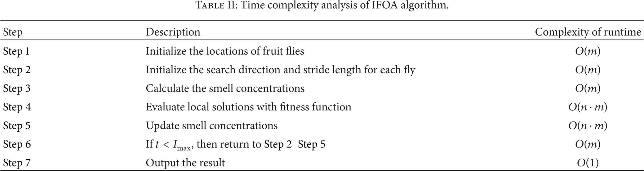
From the basic steps of IFOA in Table 11, it can be seen that after I_max generations, the time complexity of the IFOA can be estimated by the formula

T_{complexity} (n) = O (I_{\max} \cdot n \cdot m) .

(15)

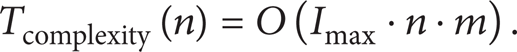
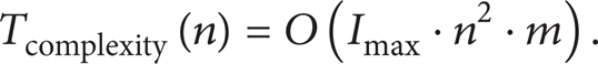
Compared with formula ((15)), the time complexity of the basic ACO is estimated by formula ((16)) [17, 18], and then we can conclude that the IFOA needs much less time than ACO in the same scale computing problems of discrete optimization, for example, TSP or path planning. Consider

T_{complexity} (n) = O (I_{\max} \cdot n^{2} \cdot m) .

(16)

Although the novel IFOA has faster convergence than ACO, the IFOA seems to fall more easily into a local optimum and premature convergence, and then the stability and accuracy are weaker than ACO too. The reason depends on the different mechanism of feedback between IFOA and ACO. As we know, ACO has negative and positive feedback through the pheromone trail updating [17], but IFOA has only the negative feedback based on fitness function. Therefore, the convergence of IFOA requires further study. In terms of application, ACO is widely used in many fields and even covered all of the optimization fields, for example, image processing [19, 20], control engineering [18], aerospace [21], and so forth. Relatively, the applications of FOA have the huge space. As a young nature-inspired algorithm, the novel FOA seems like a very simple skeleton, but it may be made into all kinds of crafts [16, 22].

Basically, the path planning problems of robots are still the most important applications involving large-scale, multiobjective, and multivariable optimization problems. Besides the improved FOA introduced in this paper, there are many other solutions with various intelligence computing models. However, three-dimensional path planning problems are still very difficult to solve completely, especially in real decision-making situations.

6. Conclusions

Although the improved FOA is much simpler than the ACO, the estimation accuracies of these two algorithms for this 3D path planning trial are very close. By repeating the simulation experiments over 40 times, the gap of the actual path optimization between the two algorithms was only approximately 2.36% on average, while the time cost of the IFOA model (the improved FOA described in this paper) saved nearly 25%. In terms of the efficiency of the algorithms, we predict that the IFOA may have a shorter running time than the ACO due to structural problems in the latter. The IFOA is better designed for solving discrete optimization problems; moreover, when time efficiency is a key consideration and some accuracy can be sacrificed, the IFOA has more advantages over the traditional ACO.

Traditional nature-inspired intelligent computation models are challenged by large-scale, multiobjective, and multivariable optimization problems; therefore, mechanisms to reduce the computing complexity of those heuristic algorithms represent an important area of study. In addition to a smaller number of control variables and a lower time complexity, the structure of the FOA is concise and can be easily combined with other algorithms or engineering techniques. Of course, as one of the latest intelligent computing models based on swarm intelligence, its stability, convergence, computational complexity, and possible applications in continuous and discrete space optimization must be further explored.

Conflict of Interests

The author declares that there is no conflict of interests regarding the publication of this paper.

Footnotes

Acknowledgments

This paper is partly supported by Fundamental Research Funds for the Central Universities (no. 2013XMS03), Guangdong Province Soft Science Research Project (no. 2013B070206020), and Guangdong Province Key Laboratory Open Foundation (no. 2011A06090100101B).

References

Caroll

K. P.

McClaran

S. R.

Nelson

E. L.

, “AUV path planning: an A* approach to path planning width consideration of variable vehicle speeds and multiple, overlapping, time-dependent exclusion zones,” in Proceedings of the IEEE Symposium on AUV Technology, pp. 79–84, Washington, DC, USA, 1992.

Ellips

and Golnaz

, “Robot path planning in 3D space using binary integer programming,” Mechanical System Science and Engineering, vol. 1, pp. 26–32, 2007.

Castillo

Trujillo

, and Melin

, “Multiple objective genetic algorithms for path-planning optimization in autonomous mobile robots,” Soft Computing, vol. 11, no. 3, pp. 269–279, 2007.

Qin

Y.-Q.

Sun

D.-B.

, and Ma

, “Path planning for mobile robot based on particle swarm optimization,” Robot, vol. 26, no. 3, pp. 222–225, 2004.

Dorigo

and Gambardella

L. M.

, “Ant colony system: a cooperative learning approach to the traveling salesman problem,” IEEE Transactions on Evolutionary Computation, vol. 1, no. 1, pp. 53–66, 1997.

Penev

and Littlefair

, “Free search—a comparative analysis,” Information Sciences, vol. 172, no. 1–2, pp. 173–193, 2005.

Liu

L.-Q.

, and Dai

Y.-T.

, “Path planning of underwater vehicle in 3D space based on ant colony algorithm,” Journal of System Simulation, vol. 20, no. 14, pp. 3712–3716, 2008.

Likun

and Hongzhao

, “The application of three-dimensional path planning of wheeled robot based on adaptive ant colony system algorithm,” Mechanical Science and Technology for Aerospace Engineering, vol. 32, no. 1, pp. 54–58, 2013.

Pan

W.-T.

, “A new fruit fly optimization algorithm: taking the financial distress model as an example,” Knowledge-Based Systems, vol. 26, pp. 69–74, 2012.

10.

Pan

W.-T.

, “Using modified fruit fly optimisation algorithm to perform the function test and case studies,” Connection Science, vol. 25, no. 2–3, pp. 151–160, 2013.

11.

, and Hu

, “A novel modified fly optimization algorithm for designing the self-tuning proportional integral derivative controller,” Journal of Convergence Information Technology, vol. 7, no. 16, pp. 69–77, 2012.

12.

Sheng

and Bao

, “Fruit fly optimization algorithm based fractional order fuzzy-PID controller for electronic throttle,” Nonlinear Dynamics, vol. 73, no. 1–2, pp. 611–619, 2013.

13.

Lin

S.-J.

Chang

, and Hsu

M.-F.

, “Multiple extreme learning machines for a two-class imbalance corporate life cycle prediction,” Knowledge-Based Systems, vol. 39, pp. 214–223, 2013.

14.

Lin

S.-M.

, “Analysis of service satisfaction in web auction logistics service using a combination of Fruit fly optimization algorithm and general regression neural network,” Neural Computing and Applications, vol. 22, no. 3–4, pp. 783–791, 2013.

15.

Xiaowen

and Qing

, “Research of optimizing performance of fruit fly optimization algorithm and five kinds of intelligent algorithm,” Fire Control & Command Control, vol. 38, pp. 17–20, 2013.

16.

Wang

Zheng

X.-L.

, and Wang

S.-Y.

, “A novel binary fruit fly optimization algorithm for solving the multidimensional knapsack problem,” Knowledge-Based Systems, vol. 48, pp. 17–23, 2013.

17.

Bonabeau

Dorigo

, and Theraulaz

, Swarm Intelligence: From Natural to Artificial Systems, Oxford University Press, New York, NY, USA, 1999.

18.

Duan

Liu

Wang

, and Yu

, “Design and realization of hybrid ACO-based PID and LuGre friction compensation controller for three degree-of-freedom high precision flight simulator,” Simulation Modelling Practice and Theory, vol. 17, no. 6, pp. 1160–1169, 2009.

19.

Al-Qaheri

Mustafi

, and Banerjee

, “Digital watermarking using ant colony optimization in fractional Fourier domain,” Journal of Information Hiding and Multimedia Signal Processing, vol. 1, no. 3, pp. 179–189, 2010.

20.

Loukhaoukha

Chouinard

J.-Y.

, and Taieb

M. H.

, “Optimal image watermarking algorithm based on LWT-SVD via multi-objective ant colony optimization,” Journal of Information Hiding and Multimedia Signal Processing, vol. 2, no. 4, pp. 303–319, 2011.

21.

Duan

, and Zhou

, “UCAV path planning based on ant colony optimization and satisficing decision algorithm,” in Proceedings of the IEEE Congress on Evolutionary Computation (CEC '08), pp. 957–962, Hong Kong, June 2008.

22.

Zheng

X.-L.

Wang

, and Wang

S.-Y.

, “A novel fruit fly optimization algorithm for the semiconductor final testing scheduling problem,” Knowledge-Based Systems, vol. 57, pp. 95–103, 2014.

Three-Dimensional Path Planning of Robots in Virtual Situations Based on an Improved Fruit Fly Optimization Algorithm

Abstract

1. Introduction

2. How to Transform a Three-Dimensional Space into a Discrete Point Set for Path Planning

3. The Fruit Fly Optimization Algorithm and Strategies for Improvement

3.1. Basic Concepts and Computing Steps of FOA

3.2. Improvement Strategies for the FOA

4. Visual Neighborhood Constraints of a Robot in Search Space

5. Improving FOA and Its Simulations in Three-Dimensional Path Planning

5.1. Improvement and Simulation of the FOA Algorithm

5.2. Comparison Experiments among FOA, IFOA, and ACO in 3D Path Planning

5.3. Analysis of the Simulation Results

5.4. Explanation of the Experimental Results

6. Conclusions

Conflict of Interests

Footnotes

Acknowledgments

References