Sage Journals: Discover world-class research

Abstract

Accurately predicting the strip profile after thin-foil cold rolling is very difficult because of the thinness of the strip. In this study, a three-dimensional (3D) strip profile model was developed to improve the accuracy of a rolled thin-foil profile. The distribution of the contact pressure between rolls (i.e., the work, intermediate, and backup rolls) and the rolling pressure between the strip and work roll were calculated by using the geometric structure of a 6-high mill and boundary conditions imposed in the width direction by a numerical method. The rolling pressure distribution in the rolling direction was determined by Fleck's model of thin-foil rolling. The 3D rolled-strip profile was predicted by using the pressures in the width and rolling directions. In order to investigate the effect of the rolling speed and rise in strip temperature on the lubrication, the friction coefficient was estimated through an analytical method and experiments to test the viscosity and friction. The resulting 3D strip profile was verified by a thin-foil cold rolling test and was compared with the profile obtained using the proposed 3D model and finite element simulation.

1. Introduction

There is growing interest in modelling thin-foil rolling processes in order to increase productivity and improve surface quality. An accurate model is needed for online control of rolling and offline programs to optimize the rolling schedule. Several models of foil rolling have been developed in the last decade. The key to develop an accurate model is accurately estimating the elastic deformation of the roll.

The earliest studies on cold rolling were conducted by von Kármán [1] and Orowan [2]. In their research, they used the simple assumption that the rolls remain circular during cold rolling. Early models, such as those developed by Orowan [2] and Bland and Ford [3], were successfully used to predict the stresses in the cold rolling of a thick strip. These models were based on a circular arc of contact and used Hitchcock's formula [4] to predict the radius of a deformed roll. However, when these models were applied to the rolling of a thin foil, where the roll was far from circular, convergence problems were experienced.

Domanti et al. [5] applied the model to thin strip and temper rolling and modelled the roll elasticity by using the influence functions for circular rolls described by Jortner et al. [6]. They reported that each calculation required only a few seconds, but the severity of the roll flattening was unclear during the calculation time. Domanti et al. then proposed a new algorithm [7] using the theory proposed by Greenwood [8] to solve the contact pressure in the flat region. The solutions were very similar to those obtained by Fleck et al. [9], but the execution times of the former were much shorter.

Fleck et al. [9] and Fleck and Johnson [10] departed from the traditional assumption that the rolls remain circular when deformed and instead assumed that, during the deformation process, the roll profile includes a central flattened region. In the Fleck and Johnson model, the pressure is considered to be near-Hertzian.

The Fleck et al. model splits the roll bite into several regions according to the elastic or plastic deformation of the strip under the assumption of slip or no-slip conditions between the strip and roll. The thin-foil cold rolling model proposed by Fleck et al. [9, 10] assumes a number of zones with the actual number depending on the rolling behaviour regime. The different zones are as follows: (A) an elastic loading zone at the start of the roll gap, (B) a plastic reduction zone with backward slip, (C) a central flattened region with no slip, (D) another plastic reduction zone with forward slip, and (E) an elastic unloading zone at the end of the roll gap. The elastic deformation of the roll is then calculated by the half-space solution for s distributed contact pressures. The boundaries between the regions are solved by the Newton-Raphson scheme to satisfy the continuity and boundary conditions. This procedure is repeated until convergence is obtained. Dixon and Yuen [11] applied this model to foil rolling with high reduction and temper rolling with minimum reduction.

The properties of the rolling lubricant also need to be estimated for thin-foil cold rolling. Because the strip is very thin, the rolling lubricant has a very large impact on the thin-foil cold rolling process. Kojima et al. [12] studied and calculated the interface temperature in cold rolling, whereas Lin and Houng [13] analysed the thermal effects under full hydrodynamic lubrication. Wilson and Mahdavian [14] developed a thermal Reynolds equation which considers viscosity variations across the lubricant film thickness, where conduction is the dominant mode of heat transfer in the lubricant. Le and Sutcliffe [15] and Zhang [16], who proposed the slab method, focused on two-dimensional (2D) deformation in thin-foil cold rolling.

In this study, a three-dimensional strip profile model was developed which uses the rolling pressures in the width and rolling directions for the continuous thin-foil cold rolling process. The pressure distribution between the rolls and the rolling pressure between the strip and work roll are calculated by using the geometric structure of the 6-high mill and the boundary conditions imposed in the width direction by a numerical method. The rolling pressure distribution in the rolling direction is determined by Fleck's thin-foil rolling model. The lubrication effect was estimated through an analytical method and experiments to measure the viscosity and friction in order to improve the accuracy of the estimated rolled thin-foil profile. The resulting three-dimensional (3D) strip profiles were compared with those obtained from thin-foil cold rolling finite element (FE) simulations and experiments.

2. Elastic Deformation as Rolled-Strip Profile in Thin-Foil Cold Rolling

Most of the theoretical basis of this study is taken directly from Fleck et al. [9]. Consider a slab element of the strip's thickness, as shown in Figure 1. Consider

b (x) = - \frac{2}{π E_{R}^{*}} \int_{- x_{a}}^{x_{d}} p (s) \ln | \frac{s + x_{a}}{s - x} | d s .

(1)

Figure 1:

Schematic of noncircular roll for thin-foil cold rolling.

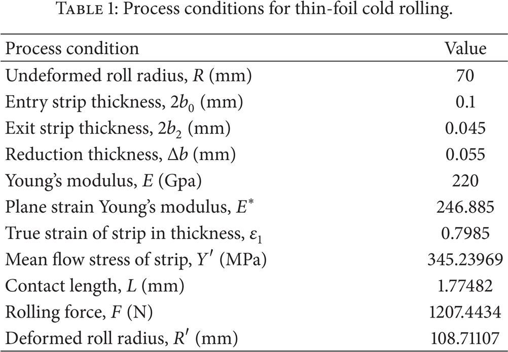
Using the above Fleck's model, we obtained the roll shape deformed by thin-foil cold rolling. Table 1 presents the process conditions for thin-foil cold rolling. The strip material was Cu-Fe-P alloy, and the initial strip size was 0.1 mm. Table 2 lists the chemical compositions of the foil measured by the inductively coupled plasma method.

Table 1:

Process conditions for thin-foil cold rolling.

Process condition	Value

Undeformed roll radius, R (mm)	70
Entry strip thickness, 2b₀ (mm)	0.1
Exit strip thickness, 2b₂ (mm)	0.045
Reduction thickness, Δb (mm)	0.055
Young's modulus, E (Gpa)	220
Plane strain Young's modulus, E^*	246.885
True strain of strip in thickness, ε₁	0.7985
Mean flow stress of strip, Y′ (MPa)	345.23969
Contact length, L (mm)	1.77482
Rolling force, F (N)	1207.4434
Deformed roll radius, R′ (mm)	108.71107

Table 2:

Chemical composition of Cu-Fe-P foil (wt%).

Element	Fe	P	Zn	Sn	Cu

Composition	0.11	0.028	0.007	0.003	Bal.

The effective stress-strain curve for the initial strip obtained through the tensile test is as follows:

\bar{σ} = 504.42 \cdot {\bar{ε}}^{0.3811} [MPa],

(2)

where $\bar{σ}$ is the effective stress and $\bar{ε}$ is the effective strain.

Table 3 lists the position of each zone in thin-foil cold rolling. The exit thicknesses of the strip, reduction ratio, and flattened roll radius were 0.045, 0.55, and 108.711 mm, respectively. The position of each zone was calculated using the MATLAB program. Figure 2 shows the deformation of the roll in thin-foil cold rolling. A deformed noncircular roll was obtained; the total deformation in the width direction can be calculated on the basis of this result.

Table 3:

Position of each zone in thin-foil cold rolling.

Point each zone	Position (mm)

a ₀	−3.12761
x _A	−2.41179
x _B	−2.09022
x _C	1.56298
x _D	2.19345
a ₂	2.83183

Figure 2:

Deformation of roll in thin-foil cold rolling.

3. Lubrication Film Thickness in Thin-Foil Cold Rolling

Owing to the extreme thinness of the rolling strip, the lubrication film thickness in thin-foil cold rolling should not be neglected for accurate prediction of the rolled-strip profile. Moreover, the lubricant film thickness is greatly influenced by the viscosity of the lubricant during the cold rolling process.

3.1. Estimation of Temperature according to Rolling Speed

The temperatures developed during the rolling process influence the lubrication conditions and the properties of the final product. Thus, the temperatures generated during plastic deformation greatly influence the productivity of the rolling process. The magnitudes and distribution of the temperatures depend mainly on the following:

initial strip and tool temperatures;

heat generated by plastic deformation and friction at the roll/strip interface;

heat transfer between the deforming material and rolls and that between the material and environment.

In the thin-foil cold rolling process, which does not use large amounts of coolants, heat losses to the environment through radiation and conduction can be neglected. Thus, the maximum instantaneous temperature of the lubricant in cold rolling T_A can be estimated by

T_{A} = T_{0} + T_{d \max} + T_{f \max},

(3)

where T₀ is the initial lubricant temperature, T_dmax is the temperature increase due to plastic deformation, and T_fmax is the temperature increase due to interface friction.

By substituting the appropriate mean value for the two heat sources (i.e., plastic deformation and interface friction), an approximation formula for the maximum interface temperature rise is obtained [12]. The maximum temperature rise due to plastic deformation is calculated as follows:

T_{d \max} = \frac{2 k}{ρ_{s} C_{s}} \ln (\frac{1}{1 - r}) \frac{β}{β + \coth (χ)},

(4)

where $β = (λ_{s} / λ_{r}) \sqrt{a_{r} / a_{s}}$ , $χ = b_{m} / 2 \sqrt{a_{s} t_{c}} = b_{m} \sqrt{v_{r}} / 2 \sqrt{a_{s} L^{'}}$ , t_c = L′/v_r. k is the material constant of the strip, r_s is the density of the strip, C_s is the specific heat of the strip, and r is the reduction ratio. λ_s and λ_r are the thermal conductivities of the strip and roll, respectively. a_s and a_r are the thermal diffusivities of the strip and roll, respectively. b_m is the average thickness of the strip, t_c is the contact time, v_r is the velocity of the roll, and L′ is the contact length between the strip and roll.

The maximum temperature rise due to friction is calculated as follows:

T_{f \max} = q_{f m} \frac{\sqrt{a_{s}}}{λ_{s}} \cdot \frac{β \sqrt{L^{'} / v_{r}}}{1 + β \tanh (χ)},

(5)

where

\begin{matrix} q_{f m} = μ p_{m} {| v_{r} - v_{s} |}_{m}, {| v_{r} - v_{s} |}_{m} = \frac{r (4 - 3 r)}{16 (1 - r)}, \\ p_{m} = \frac{1}{3} [2 k + 2 \cdot \frac{2 k b_{m}}{μ L^{'}} {\exp (\frac{μ L^{'}}{b_{m}}) - 1}] = \frac{2 k}{3} [1 + \frac{2}{(μ / α)} \cdot \frac{3 r}{3 - 2 r} [ex p {(\frac{μ}{α}) \frac{3 r}{3 - 2 r}} - 1]], \end{matrix}

(6)

μ is the friction coefficient in the cold rolling process, and α is the bite angle.

Table 4 lists the thin-foil cold rolling conditions used to calculate the strip temperature. The strip material was a Cu-Fe-P alloy, and the initial thickness and reduction ratio were 0.1 mm and 0.55, respectively. Figure 3 shows the variation in T_dmax with the roll speed. The roll speed was proportional to the temperature rise caused by plastic deformation.

Table 4:

Thin-foil cold rolling conditions for calculation of strip temperature.

Condition	Value

Material constant, k (MPa)	504.42
Mean thickness of strip, b_m (mm)	0.07
Contact length, L′ (mm)	5.96

Figure 3:

Variation in T_dmax with roll speed.

Table 5 describes the temperature rise caused by plastic deformation and friction. At the mean roll speed of 2400 mm/s, the temperature rise due to plastic deformation T_dmax and that due to friction T_fmax were calculated to be 27.10 and 0.96°C, respectively, using the approximation formula. Thus, the lubricant temperature rise was approximately 46.57°C. In the actual experiment, the lubricant temperature was measured to be 49.5°C with a noncontact infrared thermometer. The result obtained using the approximation formula was very similar to the actual result of the experiment.

Table 5:

Temperature rise due to plastic deformation and friction.

Items	Value

Initial temperature of lubrication, T₀ (°C)	18.5
The temperature rise in plastic deformation, T_dmax (°C)	27.10488878
The temperature rise in friction, T_fmax (°C)	0.960494871
Total temperature rise, T_A (°C)	46.57
The temperature of lubrication in experiment, T_R (°C)	49.5

3.2. Estimation of Viscosity according to Strip Temperature

Estimating the rolling strip temperature rise is important to predict the rolling lubricant viscosity in thin-foil cold rolling. The viscosity variation due to the rolling temperature rise also leads to variations in the friction coefficient. In this study, the variation in the lubricant viscosity with the temperature rise in the roll gap during the rolling process was predicted. In addition, the friction coefficient was determined from the predicted lubricant viscosity.

Lubrication in metal forming can reduce energy consumption and improve the product quality; hence, it is widely applied in cold strip rolling. With lubricants, the coefficient of friction between the strip and roll decreases and becomes speed dependent. Depending on the rolling conditions, the roll-strip gap can have different lubrication mechanisms. In cold rolling, the friction coefficient is related to the lubricant viscosity. In particular, the viscosity variation with temperature and pressure is given by Barus’ model:

η = η_{0} \exp [α p - γ (T - T_{0})],

(7)

where η is the lubricant viscosity, η₀ is the lubricant viscosity at ambient temperature, α is the viscosity pressure factor, and γ is the fraction of the plastic work converted to heat. T and T₀ are the lubricant and ambient temperatures, respectively. In this study, the effect of pressure was neglected because the effect of lubricant viscosity on the rolling pressure is very small. However, the effect of viscosity on temperature is significant. Therefore, the viscosity variation based on temperature variations was estimated by using a Vibro viscometer.

Viscosity is a measure of the tendency of a lubricant to resist flow; this is more correctly termed the coefficient of viscosity η. It is the ratio of the shear stress to the shear rate at a simple steady shear rate. When the viscosity of a lubricant remains constant for different shear rates, the lubricant is a Newtonian fluid. The SV-10 Vibro viscometer uses a constant frequency of 30 Hz as well as a constant amplitude. There is a damping effect related to the viscosity of the lubricant, which reduces the amplitude; thus, the power required to keep the sensors vibrating at the original amplitude is measured and converted into viscosity.

The viscosity measurement test was carried out using the SV-10 equipment. The lubricant was heated from 23°C (room temperature) to 85°C to measure the viscosity in boiling water.

Figure 4 shows the viscosity variation with the lubricant temperature. The initial viscosity at room temperature was 8.53 × 10⁻³ Pa·s, and the lubricant temperature was found to be inversely proportional to the lubricant viscosity. The relationship between the lubricant temperature and viscosity can be expressed by an exponential equation:

η = 0.0015 + 0.02014 \times \exp (- \frac{T_{L}}{22.79896}) [Pa·s],

(8)

where T_L is the lubricant temperature.

Figure 4:

Variation in viscosity variation with lubrication temperature.

The viscosity of the lubricant in thin-foil cold rolling was predicted using (8). When the calculated lubricant temperature was 46.57°C, as given in Table 5, the viscosity of the lubricant was determined to be 4.11 × 10⁻³ Pa·s, as shown in Figure 4.

3.3. Estimation of Friction Coefficient according to Viscosity of the Lubricant

As shown in Figure 4, we estimated the viscosity variation according to the lubricant temperature. In this study, the friction coefficient for thin-foil cold rolling was estimated according to the viscosity of the lubricant. While the strip is rolling, friction between the strip and roll and the plastic deformation of the strip are caused by the increase in heat produced by the lubricant in the cold rolling process. The heat increase leads to variations in the lubricant viscosity. In addition, variations in the friction coefficient are affected by the viscosity. Therefore, friction coefficient variations must be estimated according to the lubricant viscosity for accurate prediction of the strip profile in thin-foil cold rolling.

The pin and disk materials were SKH-51 and Cu-Fe-P alloy, respectively. The rotation speed and compression force were set to 460 rpm (rolling speed 150 m/min = 460 rpm) and 500 N, respectively. The experimental lubricant temperature range was 20–135°C. Table 6 lists the friction coefficients for different lubricant temperatures. To obtain the friction coefficient, the viscosity variation with temperature was calculated using (8). In addition, the friction coefficients were obtained through the pin-on-disk test. Figure 5 shows the relation between the temperature, viscosity, and friction coefficient of the lubricant. The test results showed that the friction coefficients tended to increase with the lubricant temperature.

Table 6:

Friction coefficients for different lubricant temperatures.

Lubricant temp. (°C)	Viscosity (Pa·s)	Friction coefficient

20 (room temperature)	8.23E − 03	0.0333
45	4.30E − 03	0.0355
60	2.95E − 03	0.0387
75	2.25E − 03	0.04
90	1.89E − 03	0.0441
105	1.70E − 03	0.045
120	1.60E − 03	0.0468
135	1.55E − 03	0.0473

Figure 5:

Relation between temperature, viscosity, and friction coefficient of lubricant.

When the rotation speed (N) and force (P) are constant and the lubricant viscosity (η) is inversely proportional to the friction coefficient, the relationship between the lubricant viscosity and friction coefficient can be expressed by the following exponential equation:

μ = 0.03363 + 0.0469 \cdot \exp (- 879.7365 \times \frac{η \cdot N}{P}),

(9)

where η is the lubricant viscosity, N is the rotation speed, and P is the compression force. Using (9), we obtained the friction coefficient between the roll and strip during the thin-foil rolling process. We then used the obtained friction coefficient to calculate the rolled-strip profile.

3.4. Calculation of Lubrication Film Thickness

Using the previous results, the lubrication film thickness was obtained for the thin-foil cold rolling process. Figure 6 shows the elastohydrodynamic lubrication of the roll. The film thickness is determined from Reynolds's equation for a steady 2D flow in a thin lubricating film:

\frac{d p}{d x} = 6 η (V_{1} + V_{2}) (\frac{h - h^{*}}{h^{3}}),

(10)

where [17]

h^{*} = 1.417 {(\frac{η_{0} (V_{1} + V_{2})}{p^{'}})}^{3 / 4} \frac{\sqrt{R}}{{(a_{0} + a_{2})}^{1 / 4}} .

(11)

Equation (10) is valid for the elastohydrodynamic lubrication of rollers and is based on the Hertzian pressure distribution and the fact that Reynolds's equation demands that the film must be nearly parallel to the flattened roll in the high-pressure region. In this theory, p′ is the pressure at a point in the entry zone where the converging film starts becoming parallel. The minimum thickness h_min, which was observed at the exit constriction, was found to be 80% of h^*.

Figure 6:

Elastohydrodynamic lubrication of roll.

Figure 7 shows the lubricant film thickness according to the width length. The overall lubricant film thickness was much smaller than the strip thickness, and it gradually increased from the edge towards the centre. These results were applied to accurately predict the rolled-strip profile in thin-foil cold rolling.

Figure 7:

Lubricant film thickness according to width length.

4. Prediction of 3D Strip Profile Using 6-High Mill in Thin-Foil Rolling

4.1. Analysis Procedure for Prediction of 3D Strip Profile

The 2D deformed roll shape in the rolling direction was calculated using Fleck's model. The contact and rolling pressures in the width direction were obtained by a numerical method for a 6-high mill [18]. However, accurately predicting the strip profile in thin-foil rolling by using 2D models which consider the rolling and width directions is difficult because of the extreme thinness of the strip. In particular, predicting the strip edge drop is very difficult.

In this study, the previous prediction results obtained for the rolling and width directions were combined to determine the 3D strip profile model [18 –20]. We can calculate the 3D strip profile with Fleck's model while using the rolling pressure in the 6-high mill. Figure 8 shows the 3D strip profile model which uses the rolling force predicted by the numerical model. The contact and rolling forces were calculated from the force and moment equilibrium equations, as shown in Figure 8(a), and the work roll deformation in the roll gap was obtained by using the calculated rolling force p(i), as shown in Figure 8(b).

Figure 8:

3D strip profile model predicted by numerical model using rolling force: (a) distributions of contact and rolling forces; (b) deformation model of strip in roll gap.

4.2. Prediction of Rolling Force in Width Direction

In Figure 8(a), the rolls are overhanging cylindrical beams for both supports. L₄ is the total length, L₁ is the barrel length, and L₂ and L₃ are the supported points. Table 7 presents the conditions for the thin-foil cold rolling process. The rolling material was a copper alloy with a strip width of 600 mm; the IMR and WR bender forces were equal to 128 kgf, and the rolling mill was a 6-high mill without shifting. The initial thickness was 0.1 mm, and the reduction ratio was 55%. The rolling 6-high mill had a pair of BURs, IMRs, and WRs. Under the conditions for thin-foil cold rolling described in Table 7, the contact force was calculated by a numerical method. The distribution of the rolling force was obtained from the calculated contact force.

Table 7:

Conditions for thin-foil cold rolling.

Condition		Value

Material		Cu-Fe-P (copper alloy)
Initial thickness (mm)		0.1
Target thickness (mm)		0.045
Strip width length (mm)		600
IMR bender force (Kgf)		128
WR bender force (Kgf)		128
Roll (mm)	BUR	D 630 × L₁ 835 × L₄ 2274.2
	IMR	D 300 × L₁ 890 × L₄ 2550
	WR	D 140 × L₁ 850 × L₄ 1485

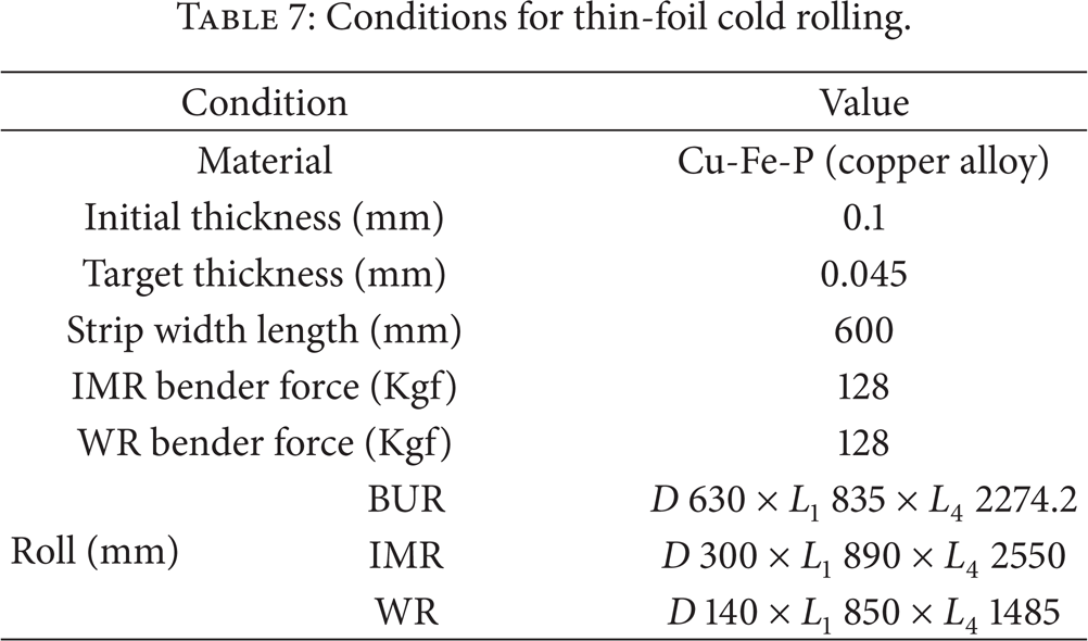
Figure 9 shows the distribution of the rolling force p(i) in the width direction. The rolling force was calculated in accordance with the contact forces, and the rolling force at the width edge was high relative to those at other positions. Therefore, edge drop appears to occur because of the high rolling force at the width edge.

Figure 9:

Distribution of p(i) in width direction.

4.3. 3D Elastic Deformation of Work Roll in Roll Gap

Figure 10 shows the flattening roll radius for various values of p(i). The roll flattening radii for the rolling force at each width position were calculated with Hitchcock's equation. The contact length at each width position in the rolling direction was obtained according to Fleck's theory using the flattening roll radius.

Figure 10:

Flattening roll radius according to rolling force p(i).

Figure 11 shows the 3D elastic deformation of WR in thin-foil cold rolling. Fleck's model was used to predict the strip profile in the roll gap in the width direction. The strip shape in the roll gap was noncircular. Based on this result, the rolled-strip profile can be obtained along the width direction.

Figure 11:

3D elastic deformation of WR in thin-foil cold rolling.

4.4. Result of Thin-Foil Cold Rolling Experiment

In order to verify the 3D strip profile model, a cold rolling experiment was carried out using the 6-high mill. The strip material was the copper alloy Cu-Fe-P. The initial thickness of the strip, target thickness, and strip width length were 0.1, 0.045, and 600 mm, respectively, and the IMR and BUR bender forces were each set to 128 kgf.

The 6-high mill was introduced to give a small area of contact when excessive pressure is the problem. This is achieved through the use of small working rolls which are supported by supporting rolls to prevent bending. Using the 6-high mill, we produced a rolled thin copper foil with a width of 600 mm. Figure 12 compares the experimental and numerical analyses of the thin strip profiles. For verification of the calculated strip shape using the 3D strip profile model, the FE simulation and experimental results were compared. Based on these comparisons, the experimentally determined rolled-strip profile was inferred to be very similar to the profile predicted using the 3D strip profile model. In particular, inhomogeneous deformation such as edge drop during cold rolling can be accurately predicted.

Figure 12:

Comparison of experimental and numerical analysis results for thin strip profiles.

5. Application of 3D Strip Profile Model in Thin-Foil Rolling Cold Rolling

5.1. Application of Strip Profile Model

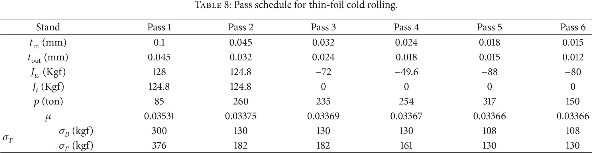
To predict the strip profile from thin-foil rolling, we applied the 3D strip profile model in Section 4. Table 8 presents the pass schedule for thin-foil cold rolling. The rolling equipment was a reverse-type 6-high mill. Six passes were performed in total, and the initial thickness and thickness of the final pass were 0.1 and 0.012 mm, respectively. The friction coefficient was calculated using (9). Figure 13 shows the distribution of the contact force in thin-foil cold rolling for each pass. The strip in the roll gap was noncircular from the centre to the edge in the width direction.

Table 8:

Pass schedule for thin-foil cold rolling.

Stand		Pass 1	Pass 2	Pass 3	Pass 4	Pass 5	Pass 6

t_in (mm)		0.1	0.045	0.032	0.024	0.018	0.015
t_out (mm)		0.045	0.032	0.024	0.018	0.015	0.012
J_w (Kgf)		128	124.8	−72	−49.6	−88	−80
J_i (Kgf)		124.8	124.8	0	0	0	0
p (ton)		85	260	235	254	317	150
μ		0.03531	0.03375	0.03369	0.03367	0.03366	0.03366
σ_T	σ_B (kgf)	300	130	130	130	108	108
σ_T	σ_F (kgf)	376	182	182	161	130	130

Figure 13:

Distribution of contact force in thin-foil cold rolling for each pass: (a) pass 1; (b) pass 2; (c) pass 3; (d) pass 4; (e) pass 5; (f) pass 6.

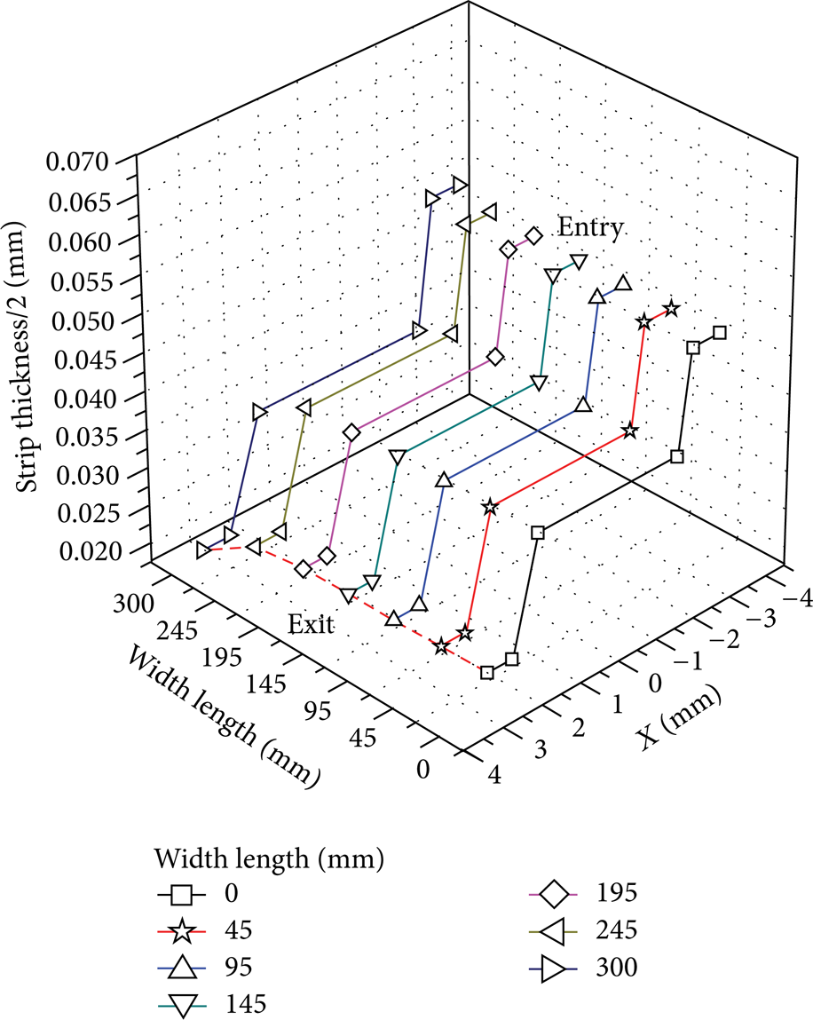
The rolled-strip profiles were calculated from the contact forces. The strip profile in the roll gap was calculated by the 3D strip profile model using the obtained contact forces. Figure 14 shows the distribution of the strip profiles in the roll gap for each pass. The strip profile in the roll gap was calculated in the width direction using the 3D strip profile model. The resultant strip in the roll gap was noncircular.

Figure 14:

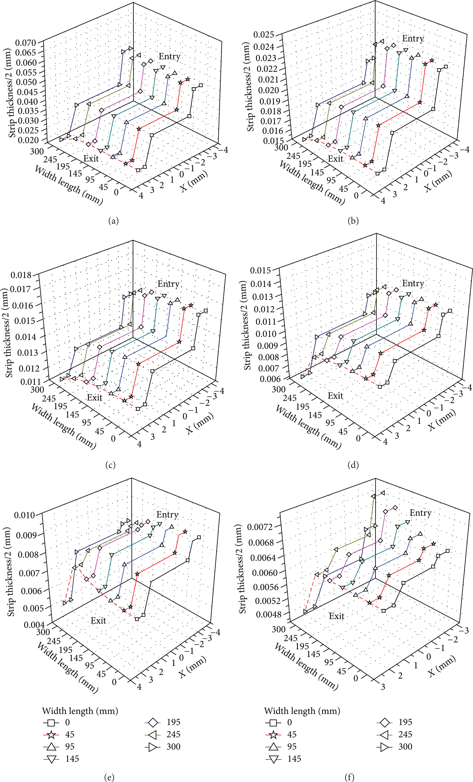
Distribution of strip profile in roll gap for each pass: (a) pass 1; (b) pass 2; (c) pass 3; (d) pass 4; (e) pass 5; (f) pass 6.

5.2. Verification of Strip Profile Model

For verification of the 3D strip profile model, FE simulations and experiments were carried out on a Cu-Fe-P strip. Table 8 presents the rolling conditions for the evaluation of the rolled-strip profile. Six passes were performed in total, and a 6-high mill without IMR shifting was used for the thin-foil rolling equipment. In the FE simulation model for elastic analysis of rolls in the thin-foil rolling, half of the model was assumed to be symmetrical to the other half. Figure 15 shows the FE simulation results for roll deformation after each pass with thin-foil cold rolling. The sizes of the rollers in the FE simulation were the same as those given in Table 7. In the results, the elastic deformations of each roll were bilaterally symmetrical, and the approximate elastic deformation was less than 1 μm. However, the edge drop along the width direction could not be accurately predicted.

Figure 15:

FE simulation results of roll deformation for each pass in thin-foil rolling: (a) pass 1; (b) pass 2; (c) pass 3; (d) pass 4; (e) pass 5; (f) pass 6.

The rolling conditions were the same as those listed in Table 8. Figure 16 compares the rolled-strip profiles from FE simulations, the actual test, and the 3D model. These results were used to verify the 3D strip profile model applied to thin-foil cold rolling. The 3D strip profile model was very similar to the FE simulation results at the centre of the width but different toward the end of the width, such as the edge drop. The rolled-strip profile predicted by the 3D strip profile model was similar to that obtained from the experiment. In particular, the edge drop at the end of the strip width was accurately predicted for thin-foil cold rolling. Thus, we confirmed that the 3D strip profile model can be applied to the thin-foil rolling process.

Figure 16:

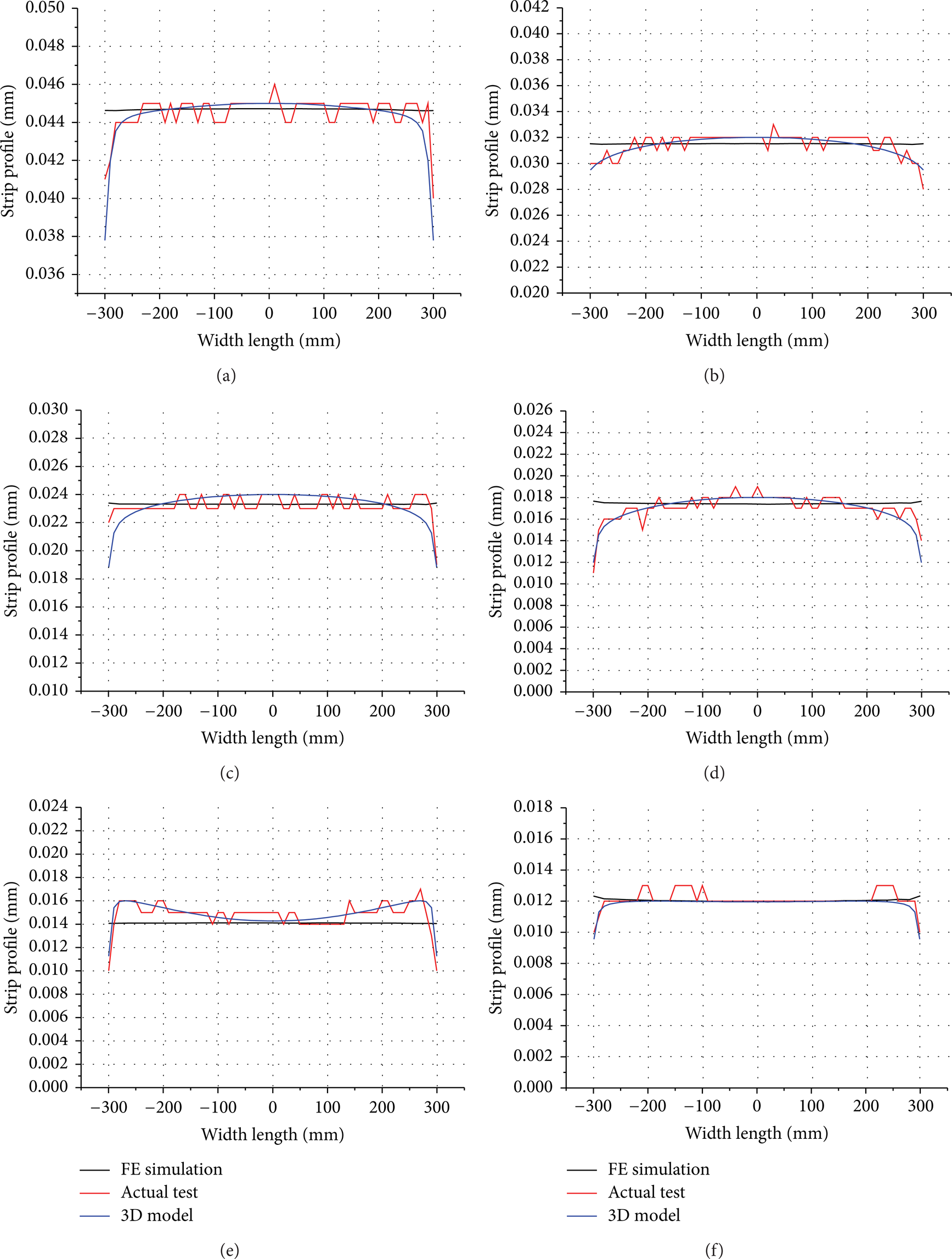
Comparison of rolled-strip profiles between FE simulation, actual test, and 3D model: (a) pass 1; (b) pass 2; (c) pass 3; (d) pass 4; (e) pass 5; (f) pass 6.

6. Conclusions

In this study, a 3D strip profile model using thin-foil rolling theory and a numerical model of a 6-high mill was developed. The results were compared with those of FE simulations and actual thin-foil cold rolling tests. The main findings are summarised below.

A deformed noncircular roll shape was obtained in thin-foil cold rolling using Fleck's model, and the total deformed roll shape in the width direction was calculated on the basis of this result.

The lubricant temperature in the thin-foil cold rolling process was calculated according to the rolling speed, and the lubricant viscosity was obtained according to the predicted strip temperature using a Vibro viscometer. The friction coefficient in the roll gap was estimated from the calculated lubricant viscosity by the pin-on-disk experiment.

To obtain the friction coefficient, the viscosity variation with temperature was calculated using (8), and the friction coefficients were obtained through the pin-on-disk test. When the rotation speed (N) and force (P) were constant, the lubricant friction coefficient was inversely proportional to the lubricant viscosity.

Using the previous results, the lubrication film thickness in thin-foil cold rolling was obtained. The overall lubricant film thickness was much less than the strip thickness, and it gradually increased from the centre toward the edge in the transverse direction.

In order to predict the rolled-strip profile in thin-foil cold rolling, we calculated the 3D strip profile with Fleck's model using the rolling pressure in the 6-high mill. The contact and rolling forces were calculated from the force and moment equilibrium equations, and the work roll deformation in the roll gap was calculated using the rolling force p(i).

The rolled-strip profiles of the experimental results and 3D strip profile model were compared to verify the accuracy of the 3D strip profile model applied to thin-foil cold rolling. The rolled-strip profile predicted by the 3D strip profile model was similar to the experimental profile. In particular, inhomogeneous deformation such as the edge drop at the end of the strip width was accurately predicted for thin-foil cold rolling. Thus, we confirmed that the 3D strip profile model can be applied to the thin-foil rolling process.

Conflict of Interests

The authors declare that there is no conflict of interests regarding the publication of this paper.

Footnotes

Authors’ Contribution

Sangho Lee and Kyunghun Lee contributed equally to this work.

Acknowledgments

This work was supported by the National Research Foundation of Korea (NRF) Grant funded by the Korean government (MSIP) (no. 2012R1A5A1048294) and PNU-IFAM JRC.

References

von Kármán

, “Beitrag zur theories des walzvorganges,” Zeitschrift für Angewandte, Mathematik und Mechanik, vol. 5, pp. 139–141, 1925.

Orowan

, “The calculation of roll pressure in hot and cold rolling,” Proceeding of the Institution of Mechanical Engineers, vol. 150, no. 4, pp. 140–167, 1943.

Bland

D. R.

and Ford

, “The calculation of roll force and torque in cold strip with tensions,” Proceeding of the Institution of Mechanical Engineers, vol. 159, pp. 144–163, 1948.

Hitchcock

J. H.

, Roll Neck Bearing, ASME Research Publication, Appendix 1, 1935.

Domanti

S. A.

Edwards

W. J.

Thomas

P. J.

, and Chefneux

I. L.

, “Application of foil rolling models to thin steel strip and temper rolling,” in Proceedings of the 6th International Rolling Conference, pp. 422–429, Dussedorf, Germany, 1994.

Jortner

Osterle

J. F.

, and Zorowski

C. F.

, “An analysis of cold strip rolling,” International Journal of Mechanical Sciences, vol. 2, no. 3, pp. 179–194, 1960.

Domanti

S. A.

Edwards

W. J.

, and Thomas

P. J.

, “A model for rolling and thin strip rolling,” in Proceedings of the AISE Annual Convention, Cleveland, Ohio, USA, 1994.

Greenwood

J. A.

, “An extension of the Grubin theory of elastohydrodynamic lubrication,” Journal of Physics D: Applied Physics, vol. 5, no. 12, pp. 2195–2211, 1972.

Fleck

N. A.

Johnson

K. L.

Mear

M. E.

, and Zhang

L. C.

, “Cold rolling of foil,” Proceedings of the Institution of Mechanical Engineers, B: Journal of Engineering Manufacture, vol. 206, no. 2, pp. 119–131, 1992.

10.

Fleck

N. A.

and Johnson

K. L.

, “Towards a new theory of cold rolling thin foil,” International Journal of Mechanical Sciences, vol. 29, no. 7, pp. 507–524, 1987.

11.

Dixon

A. E.

and Yuen

W. Y. D.

, “A computationally fast method to model thin strip rolling,” in Proceedings of the Computational Techniques and Application Conference, pp. 239–246, 1995.

12.

Kojima

Takeyama

, and Mizuno

, “Calculation of interface temperature in cold rolling,” The Japan Society for Technology of Plasticity, vol. 30, no. 342, pp. 1004–1009, 1989.

13.

Lin

J.-F.

and Houng

S.-C.

, “A refined model for the thermal hydrodynamic lubrication theory of high-speed rolling. Part I: effects of operating conditions,” Tribology International, vol. 24, no. 3, pp. 151–161, 1991.

14.

Wilson

W. R. D.

and Mahdavian

S. M.

, “A thermal Reynolds equation and its application in the analysis of plastohydrodynamic inlet zone,” Journal of Lubrication Technology, vol. 96, no. 4, pp. 572–578, 1974.

15.

H. R.

and Sutcliffe

M. P. F.

, “A robust model for rolling of thin strip and foil,” International Journal of Mechanical Sciences, vol. 43, no. 6, pp. 1405–1419, 2001.

16.

Zhang

L. C.

, “On the mechanism of cold rolling thin foil,” International Journal of Machine Tools and Manufacture, vol. 35, no. 3, pp. 363–372, 1995.

17.

Johnson

K. L.

, Contact Mechanics, Cambridge University Press, Cambridge, UK, 1992.

18.

Lee

S.-H.

Song

G.-H.

Lee

S.-J.

, and Kim

B.-M.

, “Study on the improved accuracy of strip profile using numerical formula model in continuous cold rolling with 6-high mill,” Journal of Mechanical Science and Technology, vol. 25, no. 8, pp. 2101–2109, 2011.

19.

Lee

S. H.

Lee

K. H.

Lee

S. B.

, and Kim

B. M.

, “Study of edge-cracking characteristics during thin-foil rolling of Cu-Fe-P strip,” International Journal of Precision Engineering and Manufacturing, vol. 14, no. 12, pp. 2109–2118, 2013.

20.

Lee

S. H.

, Study on the 3D strip profile and characteristics of edge cracking in thin foil rolling processd [Ph.D. thesis], School of Mechanical Engineering, Pusan National University, Busan, Republic of Korea, 2011.

Development of Three-Dimensional Strip Profile Model for Thin-Foil Cold Rolling

Abstract

1. Introduction

2. Elastic Deformation as Rolled-Strip Profile in Thin-Foil Cold Rolling

3. Lubrication Film Thickness in Thin-Foil Cold Rolling

3.1. Estimation of Temperature according to Rolling Speed

3.2. Estimation of Viscosity according to Strip Temperature

3.3. Estimation of Friction Coefficient according to Viscosity of the Lubricant

3.4. Calculation of Lubrication Film Thickness

4. Prediction of 3D Strip Profile Using 6-High Mill in Thin-Foil Rolling

4.1. Analysis Procedure for Prediction of 3D Strip Profile

4.2. Prediction of Rolling Force in Width Direction

4.3. 3D Elastic Deformation of Work Roll in Roll Gap

4.4. Result of Thin-Foil Cold Rolling Experiment

5. Application of 3D Strip Profile Model in Thin-Foil Rolling Cold Rolling

5.1. Application of Strip Profile Model

5.2. Verification of Strip Profile Model

6. Conclusions

Conflict of Interests

Footnotes

Authors’ Contribution

Acknowledgments

References