Sage Journals: Discover world-class research

Abstract

The interpolation technology is critical to performance of CNC and industrial robots; this paper proposes a new precision interpolation algorithm based on analysis of root cause in speed and acceleration. To satisfy continuity of speed and acceleration in interpolation process, this paper describes, respectively, variable acceleration precision interpolation of two stages and three sections. Testing shows that CNC system can be enhanced significantly by using the new fine interpolation algorithm in this paper.

1. Introduction

Actual curve is usually replaced by using uniform linear in the precision interpolation process, when arbitrary curve can be achieved by using two-level interpolation system in the process of interpolation. The ideal speed is changing in real time in the process of interpolation; however, if various linear is replaced by uniform linear, its speed and acceleration will not be continuous; there are some fluctuations for pulse output signal frequency between two rough interpolations, which cannot contribute to stable work for motor and motor drive, limit seriously acceleration and deceleration capability of the overall system, and restrict efficiency as well, while the greater impact will be imposed on the mechanical system, and mechanical system life will be shorten as well.

In order to deal with this kind of discontinuity for speed and acceleration, dynamical changes in the first level interpolation period are usually used in the industry to alleviate this disadvantage, but the method verifies that efficiency will be limited for processing larger curvature curve; this is not ideal in practical use. A new series of the precision interpolation algorithms are proposed in this paper based on analysis of root cause for speed and acceleration, which can effectively solve the above-mentioned disadvantage.

2. Realization Method for Pulse with Decimal and Decimal Speed

2.1. The Analysis of Root Cause for Fluctuation of Speed and Acceleration

The rough interpolation is enslaved to interpolation period in two-level interpolation system; position increments obtained by the rough interpolation need to be completed in every period, but the period is variable. This problem can be visually illustrated in the following examples: position unit and speed unit are separately recorded as “pulse equivalent” and “pulse equivalent” (or “interpolation period”) in uniform so as to facilitate presentation in this section. If linear speed of x-axis is set as 1.5, then per interpolation period should receive 1.5 pulses, current DDA method cannot achieve interpolation of 1.5 pulses in one period; thus the rough interpolation can give sequence of pulse numbers in per period, which is shown as 1, 2, 1, 2,…; therefore, actual pulse speed fluctuates every two periods.

This disadvantageous effect decreased by suitable eliminated preloaded modes because the preloaded modes control opportunity for appearance of the first pulse in per interpolation period. Waveforms are, respectively, shown in four situations (without using load, 1/4 load, half-load, 3/4 load, and full load) from top to bottom in Figure 1. Time interval between two pulses is fixed in the period where pulse numbers are 2; therefore, this method using preloaded mode only cannot solve this disadvantage; in other words, it is necessary to regulate pulse/speed with decimals to obtain ideal waveforms.

Figure 1:

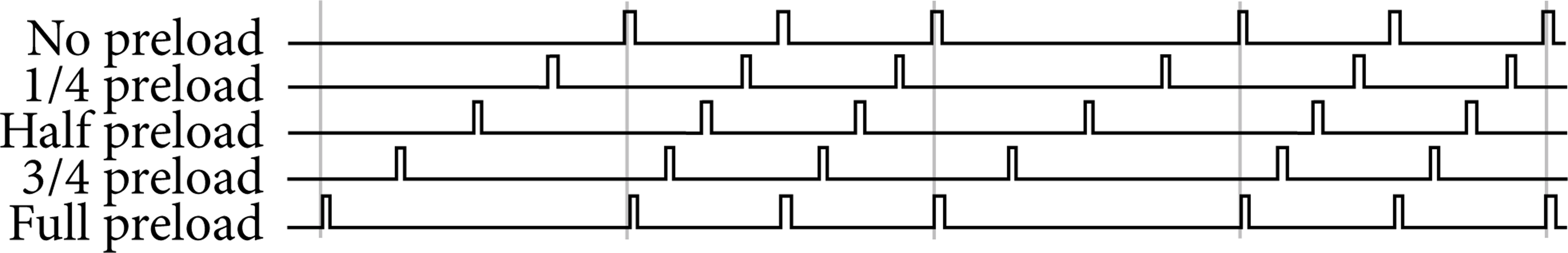
Waveforms for a variety of preloaded modes.

2.2. The Concept of Pulse with Decimal and the Decimal Speed Realization

To enable common digital circuit with decimal subdivision, decimal part should be transformed, and its transformation results should be applied to simulate DDA process in order to achieve decimal speed as well. DDA interpolator structure for realizing speed decimal is shown in Figure 2. Integer part of the speed is recorded as V_i, and its decimal part is recorded as V_f. The part within dash line is modified to achieve decimal speed compared with general DDA interpolator.

Figure 2:

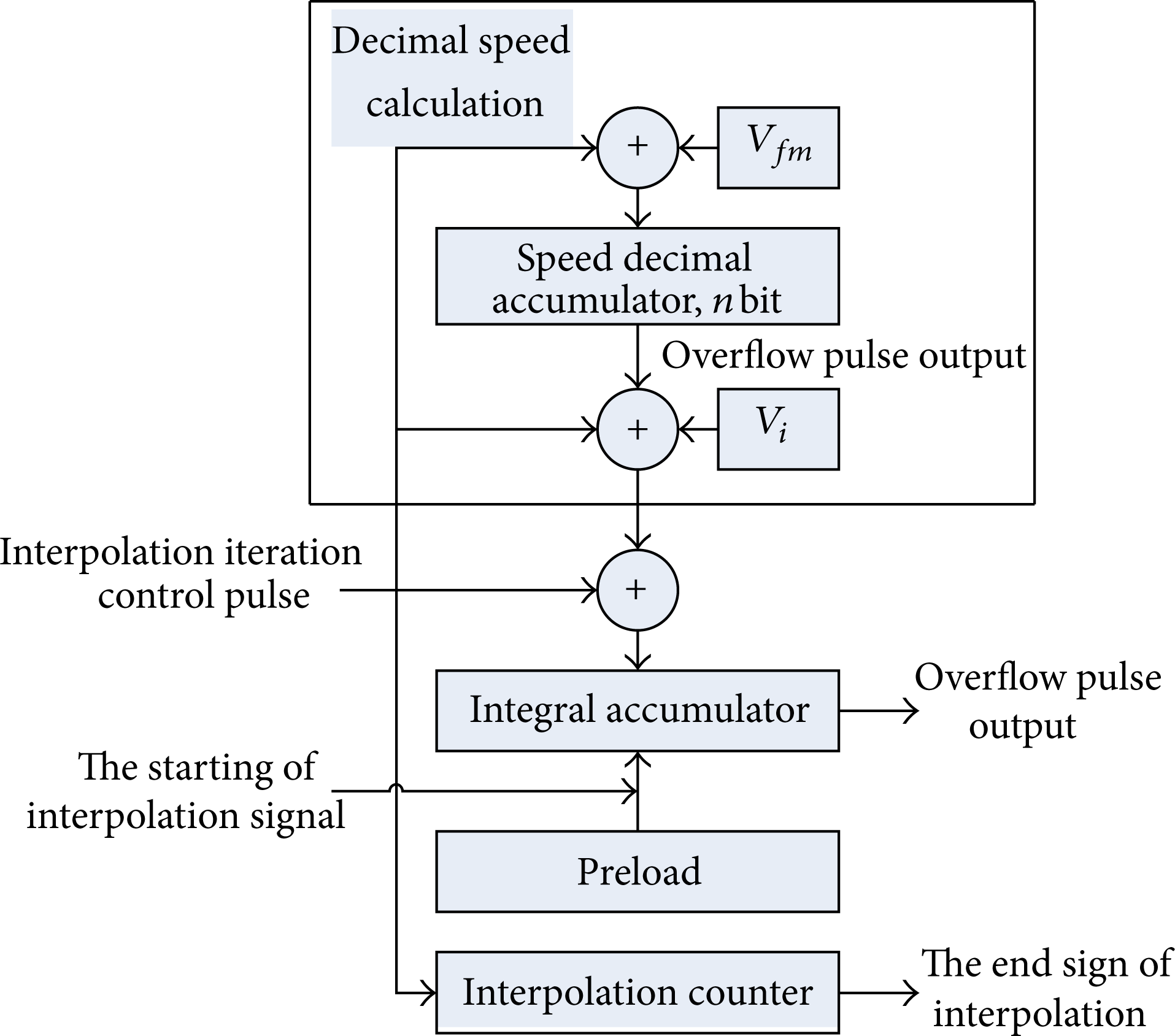
DDA interpolation structure with decimal control.

The situation that above-mentioned interpolator structure is simply used without modifying the first stage interpolation can cause error of number of pulses; in other words, position accuracy cannot be guaranteed for speed decimalization because speed in interpolation process is faster than the one without decimalization, which results in loss of pulses number; therefore, concept of pulse decimal is introduced in order to compensate for this disadvantage. In fact, pulse decimal always exists in the DDA algorithm, which is the value within integral accumulator. When an interpolation is completed, remainders within integral accumulator are exactly pulse decimal, and the preloaded values in preloaded method are similarly concrete manifestation of pulse decimal as well. Their differences are that preloaded values are not finished in the last interpolation process, but remainders are not finished in this interpolation process. The former should “owe” to the last interpolation process and the latter should “lend” to the next interpolation process within accumulator. Therefore, remainders of the last interpolation process are the same with default values in this interpolation process. By analysis of preloaded and integral remainder, the rough interpolation software can achieve full control for precision interpolation by taking advantage of remainder obtained by simulating position.

2.3. The Concept of Pulse with Decimal Realization

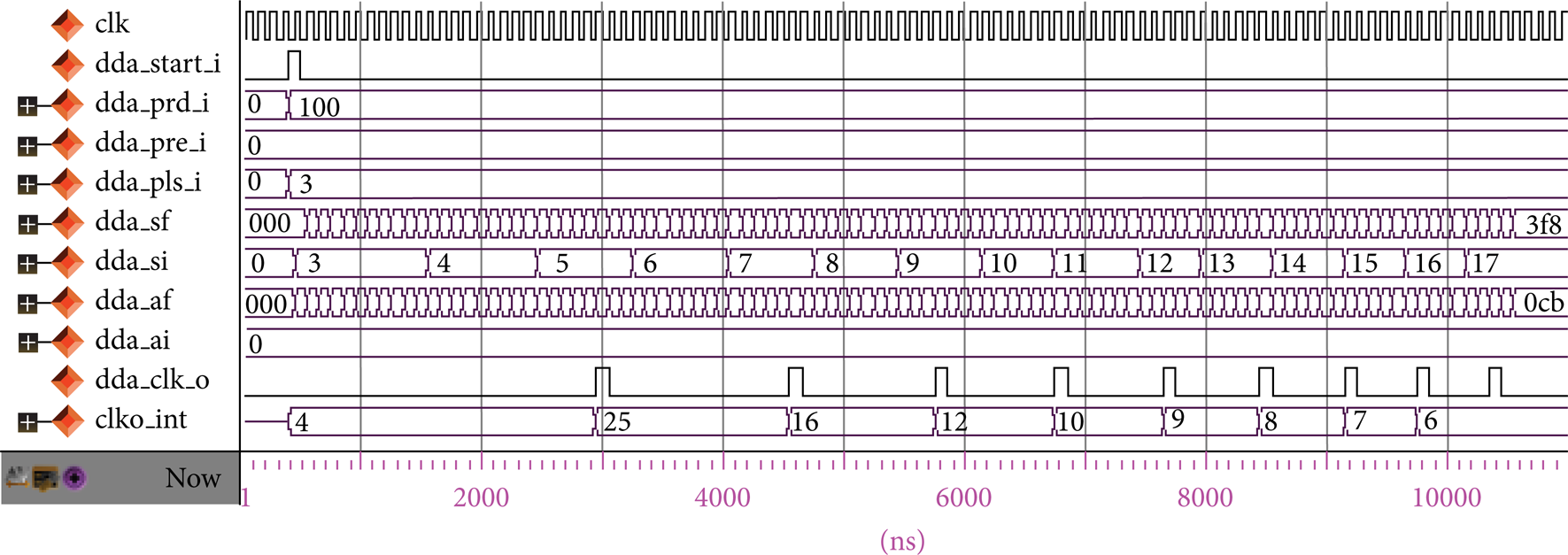
If the nth decimal section of position value by the rough interpolation is set as N, then preloaded values in the (n + 1) th cycle of integral accumulator for precision interpolation are N multiply overflow values of speed decimal accumulator; an example whose speed is 1.5 is used, whose simulation waveforms are shown in Figure 3.

Figure 3:

Speed decimal and waveform of pulse decimal.

It can be found from Figure 3 that pulses are even and number of pulses is obviously accurate. When the nth precision interpolation is completed, another example is introduced in order to illustrate better relationship between integral accumulator remainder and position value. The precision interpolation is conducted with speed sequence: 1.1, 2.2, 3.3, 4.4, 5.5, and value of position sequence is 0, 1.1, 3.3, 6.6, 11.0; preloaded values calculated by above principle are, respectively, 0, 0.1, 0.3, 0.6, 0. The simulation waveforms are shown in Figure 4.

Figure 4:

The relationship between the integral accumulator remainder and position value.

dda_acc_o is remainder value of integral accumulator. Obviously, remainder values of integral accumulator is decimal part of position value (difference between accumulator remainder and theoretical value is 1 so that code can be easy to handle and hardware resource can be saved as well).

Module uses software QuartusII 9.0 to synthesize, the device utilizes Cyclone series, logic unit occupancy quantity is 124, and running clock is above 150 MHz.

3. Research on the Precision Interpolation for Straight Line Segment in Acceleration and Deceleration Process

3.1. Method for Accelerated and Decelerated Process

Advantages for linear acceleration and deceleration algorithm are a small amount of calculation in the rough interpolation process, but its disadvantage is that acceleration without continuity results in speed curve unsmooth, which ultimately causes vibration of driving part, so this algorithm is not suitable for high speed motion control system. Exponential acceleration and deceleration algorithm has some certain advantages in starting process of acceleration and deceleration, but if the speed becomes constant after acceleration process, the situation that acceleration mutation will also arise will worsen actual motion control effect as well [1, 2]. Calculation amount is rather larger if polynomial function is applied to acceleration curve control, and polynomial can achieve desired effect by using ascending powers so as to obtain more desirable dynamic characteristics; therefore, calculation amount will exponentially grow [3, 4] by increase in polynomial degree. Acceleration and deceleration of S type introduce increase and attenuation process for acceleration so that the whole interpolation process gets smoother while calculation amount is relatively smaller, and control between acceleration region and deceleration region [5] differ from each other; therefore, S type has been widely applied.

3.2. The Concept for the Precision Interpolation in Acceleration and Deceleration Process

Realization method for speed with decimal and pulse with decimal can ensure speed continuation of connection point for rough interpolation in uniform motion but cannot be guaranteed in variable motion. As for how to ensure continuity of pulse interval between rough interpolations, or how to make speed continuous, in year 2010, Zhang et al. had proposed a method of using uniformly accelerated precision interpolation to ensure continuous speed of the fine interpolation, which has great value [6]. But acceleration and deceleration of S type are usually used in practical project to improve efficiency of acceleration and deceleration because uniform accelerated precision interpolation cannot adapt to such requirement.

This paper argues that the fundamental reason why speed is not continuous is that integrator accuracy of DDA is not enough, but this integral accuracy problem is different from the above-mentioned one. The above-mentioned integral accuracy problem without any relationship with the rough interpolation is an internal DDA problem, which is absolutely done in the precision interpolation process on the condition decimal information obtained by the precision interpolation, but pulse intervals within the precision interpolation are still invariable by only using this method.

To achieve continuous changes for pulse in the whole interpolation process, more information about the precision interpolation needs to be acquired; speed change situation based on above-mentioned analysis in acceleration and deceleration process should be analyzed in order to make pulse accurate. This paper uses the jerk precision interpolation to achieve fine interpolation in process of acceleration and deceleration of S style, which can eliminate integral errors and ensure making speed and acceleration continuous.

3.3. The Precision Interpolation for Jerk

In order to control speed in Figure 1, acceleration and jerk should be added to achieve the jerk fine interpolation. Integer part and decimal part of the acceleration are separately recorded as A_i and A_f. Integer part and decimal part of the jerk acceleration are separately recorded as J_i and J_f; therefore, new structure is shown in Figure 5.

Figure 5:

Speed control of uniform jerk DDA interpolation.

If the speed is set as 3.0, then preloaded value will be 0, acceleration will be 0.1, and jerk will be 0.001. Simulation results are shown in Figure 6. Meanwhile, dda_ai and dda_af are separately integer part and decimal part of current acceleration; obviously, pulse interval decreases faster while speed integer increases by acceleration.

Figure 6:

Output waveform of the uniform jerk DDA interpolation pulse.

The module uses software QuartusII 9.0 to synthesize, the device is Cyclone series, occupancy of logical unit is 168, and running speed is above 150 MHz.

4. Research on the Precision Interpolation for Arbitrary Curve Segment in Acceleration and Deceleration Process

4.1. The Precision Interpolation for Two Various Stages of Acceleration with Continuity of Speed

In arbitrary curve [7 –15], position increment cannot guarantee to be coincident with position increments obtained in process of the rough interpolation; only in straight line track they can be coincident with each other. Similarly, this disadvantage exists in calculating jerk acceleration as well. The disadvantage can be explained by geometry method. The area under the curve are integration value of speed and position increment, which are shown in Figure 7, starting speed point v_s, and ending speed point v_e are connected by using straight line if by using the uniform accelerated fine interpolation, and area under the line is not equal to area under the curve.

Figure 7:

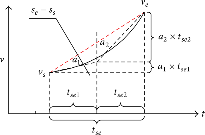
Schematic diagram of the uniformly accelerated precision interpolation for arbitrary curve.

As for realization principle and calculation method of acceleration, this paper proposes the variable two stages of acceleration precision interpolation in order to ensure positional accuracy. An acceleration switching point is set in the process of the fine interpolation when actual speed reaches speed from switching point in acceleration process, which will change into another speed, not only can it ensure accuracy of position increments, but also can achieve continuity of speed at boundary of the rough interpolation. Speed change is shown in Figure 7, and point p is the acceleration switching point in the figure.

The premise on realizing the variable two stages of accelerated precision interpolation is to obtain acceleration values through two stages style; this issue can be described as follows.

Show that starting position is s_s, end position is s_e, the first period of time is t_se1, the second period of time is t_se2, starting speed is v_s, and end speed is v_e.

Evaluate acceleration a₁ (the first period of time) and acceleration a₂ (the second period of time).

In order to ensure continuity of speed, it is necessary to satisfy the following speed formula:

v_{s} + a_{1} \times t_{s e 1} + a_{2} \times t_{s e 2} = v_{e} .

(1)

Meanwhile, in order to ensure positional accuracy, it is necessary to satisfy the following positional accuracy formula:

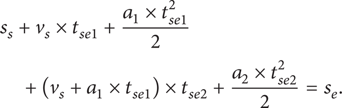
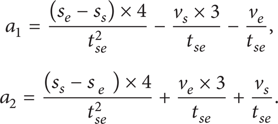
s_{s} + v_{s} \times t_{s e 1} + \frac{a_{1} \times t_{s e 1}^{2}}{2} + (v_{s} + a_{1} \times t_{s e 1}) \times t_{s e 2} + \frac{a_{2} \times t_{s e 2}^{2}}{2} = s_{e} .

(2)

Evaluating dual linear equation composed of (1) and (2), we can get acceleration value of two sections a₁ and a₂:

\begin{matrix} a_{1} = \frac{s_{e} - s_{s} - v_{s} \times t_{s e 1} - ((v_{e} \times t_{s e 2}) / 2) - ((v_{s} \times t_{s e 2}) / 2)}{(t_{s e 1}^{2} / 2) + ((t_{s e 1} \times t_{s e 2}) / 2)}, \\ a_{2} = \frac{s_{s} - s {}_{e} + v_{e} \times t_{s e 2} + v_{s} \times (t_{s e 1} / 2) + v_{e} \times (t_{s e 1} / 2)}{(t_{s e 2}^{2} / 2) + ((t_{s e 1} \times t_{s e 2}) / 2)} . \end{matrix}

(3)

In practical use circumstance, the two periods of time can be equal to simplifying the calculation. If cycle of the rough interpolation is set as t_se, then t_se1 = t_se2 = t_se/2; (3) can be rewritten as

\begin{matrix} a_{1} = \frac{(s_{e} - s_{s}) \times 4}{t_{s e}^{2}} - \frac{v_{s} \times 3}{t_{s e}} - \frac{v_{e}}{t_{s e}}, \\ a_{2} = \frac{(s_{s} - s {}_{e}) \times 4}{t_{s e}^{2}} + \frac{v_{e} \times 3}{t_{s e}} + \frac{v_{s}}{t_{s e}} . \end{matrix}

(4)

4.2. The Consecutive Three Variable Sections Acceleration Jerk Precision Interpolation of Acceleration

Realization principle and calculation method for acceleration are shown in this section. This paper introduces concept of jerk in acceleration and deceleration process of S style for some occasions that require consecutive acceleration. Division method for two stages in this paper cannot guarantee continuous acceleration, continuous speed, and positional accuracy at the same time; therefore, change process of jerk will be divided into three stages, which is shown in Figure 8; point p₁ and point p₂ are separately switching points.

Figure 8:

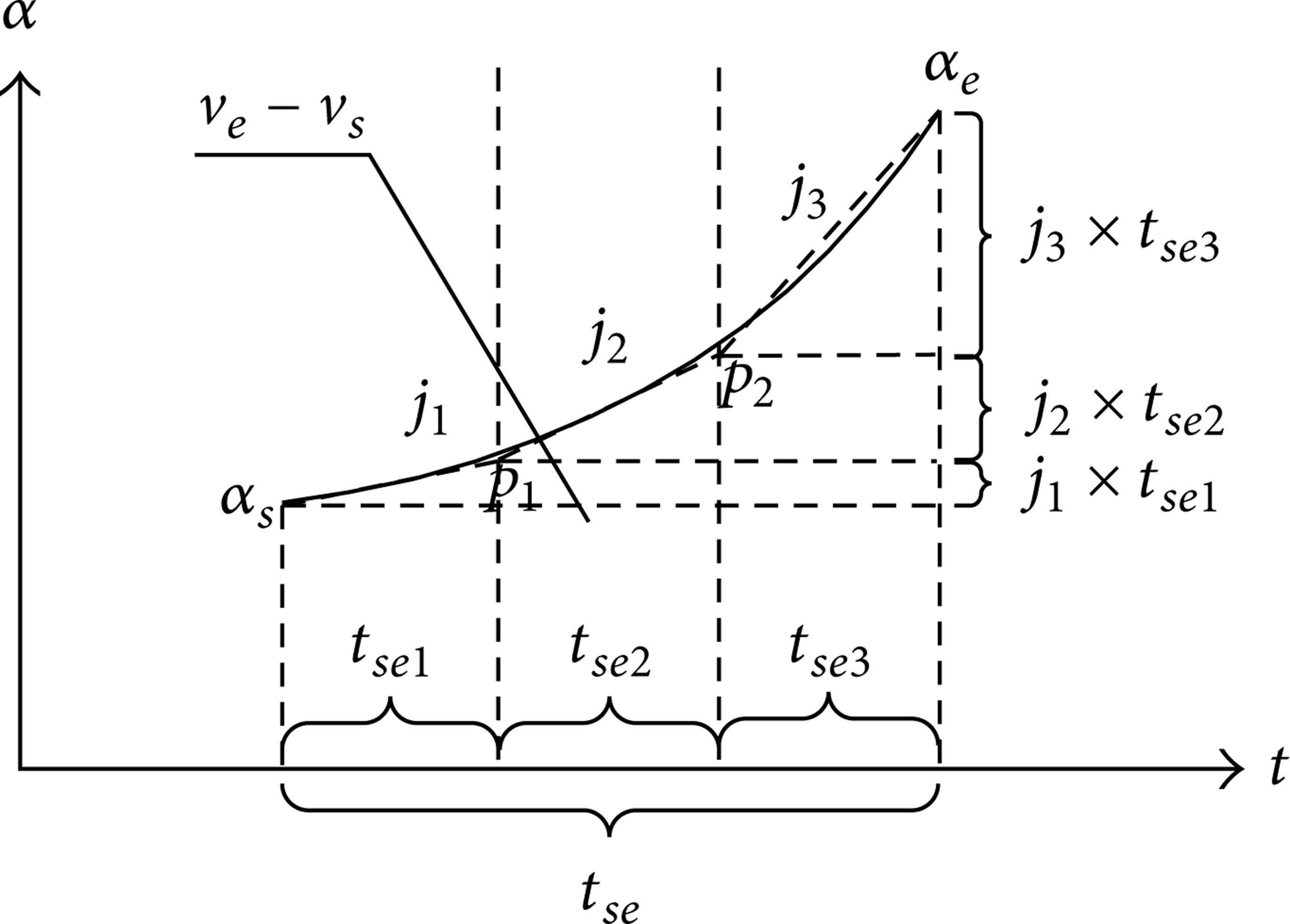
Schematic diagram of the jerk precision interpolation for arbitrary curve.

The premise on achieving three variable sections acceleration and deceleration precision interpolation is to obtain jerk value from three sections. This issue can be described as follows.

Show that starting position is s_s, end position is s_e, the first period of time is t_se1, the second period of time is t_se2, starting speed is v_s, end speed is v_e, starting acceleration is a_s, and end acceleration is a_e.

Evaluate acceleration j₁ (the first period of time), acceleration j₂ (the second period of time), and acceleration j₃ (the third period of time).

In order to ensure continuity of acceleration, it is necessary to satisfy the following acceleration formula:

a_{s} + j_{1} \times t_{s e 1} + j_{2} \times t_{s e 2} + j_{3} \times t_{s e 3} = a_{e} .

(5)

In order to facilitate speed formula derivation, acceleration expressions of three periods of time are written as follows:

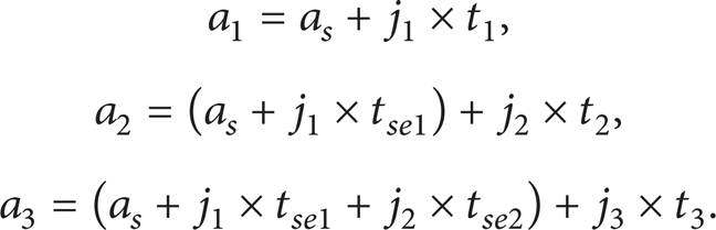
\begin{matrix} a_{1} = a_{s} + j_{1} \times t_{1}, \\ a_{2} = (a_{s} + j_{1} \times t_{s e 1}) + j_{2} \times t_{2}, \\ a_{3} = (a_{s} + j_{1} \times t_{s e 1} + j_{2} \times t_{s e 2}) + j_{3} \times t_{3} . \end{matrix}

(6)

From system (6), acceleration of the first section, the second section, and the third section are, respectively, recorded as a₁, a₂, a₃; starting time of this segment compared with the first section, the second section, and the third section is, respectively, recorded as t₁, t₂, t₃. This can be used for ensuring the formula of continuity of speed:

v_{s} + a_{s} \times t_{s e 1} + \frac{j_{1} \times t_{s e 1}^{2}}{2} + (a_{s} + j_{1} \times t_{s e 1}) \times t_{s e 2} + \frac{j_{2} \times t_{s e 2}^{2}}{2} + (a_{s} + j_{1} \times t_{s e 1} + j_{2} \times t_{s e 2}) \times t_{s e 3} + \frac{j_{3} \times t_{s e 3}^{2}}{2} = v_{e} .

(7)

Similarly, in order to facilitate position formula derivation, speed expressions of three periods of time are written as follows:

\begin{matrix} v_{1} = v_{s} + a_{s} \times t + \frac{j_{1} \times {(t_{1})}^{2}}{2}, \\ v_{2} = (v_{s} + a_{s} \times t_{s e 1} + \frac{j_{1} \times t_{s e 1}^{2}}{2}) + (a_{s} + j_{1} \times t_{s e 1}) \times t_{2} + \frac{j_{2} \times t_{2}^{2}}{2}, \\ v_{3} = (v_{s} + a_{s} \times t_{s e 1} + \frac{j_{1} \times t_{s e 1}^{2}}{2} + (a_{s} + j_{1} \times t_{s e 1}) \times t_{s e 2} + \frac{j_{2} \times t_{s e 2}^{2}}{2}) + (a_{s} + j_{1} \times t_{s e 1} + j_{2} \times t_{s e 2}) \times t_{3} + \frac{j_{3} \times t_{3}^{2}}{2} . \end{matrix}

(8)

From system (8), speed of the first section, the second section, and the third section is, respectively, recorded as v₁, v₂, v₃. From system (8), this can be used for ensuring the formula of position accuracy, so we have

\begin{matrix} s_{s} + v_{s} \times t_{s e 1} + a_{s} \times \frac{t_{s e 1}^{2}}{2} + \frac{j_{1} \times t_{s e 1}^{3}}{6} + (v_{s} + a_{s} \times t_{s e 1} + \frac{j_{1} \times t_{s e 1}^{2}}{2}) \times t_{s e 2} + (a_{s} + j_{1} \times t_{s e 1}) \\ \times \frac{t_{s e 2}^{2}}{2} + \frac{j_{2} \times t_{s e 2}^{3}}{6} + (v_{s} + a_{s} \times t_{s e 1} + \frac{j_{1} \times t_{s e 1}^{2}}{2} + (a_{s} + j_{1} \times t_{s e 1}) \times t_{s e 2} + \frac{j_{2} \times t_{s e 2}^{2}}{2}) \\ \times t_{s e 3} + (a_{s} + j_{1} \times t_{s e 1} + j_{2} \times t_{s e 2}) \\ \times \frac{t_{s e 3}^{2}}{2} + \frac{j_{3} \times t_{s e 3}^{3}}{6} = s_{e} . \end{matrix}

(9)

The ternary equations can be composed of (7), (8), and (9), so solving this equation, we can get j₁, j₂, j₃:

\begin{matrix} j_{1} = \frac{l (c f c - c g b) + h (c k b - c j c) + d (g j c - k f c)}{g a j c - e c j c + e c k b - k a f c + i c f c - i c g b}, \\ j_{2} = \frac{l (c e c - c g a) + h (c k a - c i c) + d (g i c - k e c)}{g b i c - f c i c + f c k a - k b e c + j c e c - j c g a}, \\ j_{3} = \frac{l (a f a - a e b) + h (a i b - a j a) + d (e j a - i f a)}{e c j a - g a j a + g a i b - i c f a + k a f a - k a e b} . \end{matrix}

(10)

From system (10), a, b, c, d, e, f, g, h, i, j, k, l present, respectively, the following values:

\begin{matrix} a = t_{s e 1}, b = t_{s e 2}, c = t_{s e 3}, \\ d = (a_{e} - a_{s}), \\ e = (\frac{t_{s e 1}^{2}}{2} + t_{s e 1} \times t_{s e 2} + t_{s e 1} \times t_{s e 3}), \\ f = (\frac{t_{s e 2}^{2}}{2} + t_{s e 2} \times t_{s e 3}), \\ g = \frac{t_{s e 3}^{2}}{2}, h = v_{e} - v_{s} - a_{s} \times (t_{s e 1} + t_{s e 2} + t_{s e 3}), \\ i = (\frac{t_{s e 1}^{3}}{6} + \frac{t_{s e 1}^{2}}{2} \times t_{s e 2} + \frac{t_{s e 2}^{2}}{2} \times t_{s e 1} + \frac{t_{s e 1}^{2}}{2} \times t_{s e 3} + t_{s e 1} \times t_{s e 2} \times t_{s e 3} + t_{s e 1} \times \frac{t_{s e 3}^{2}}{2}), \\ j = (\frac{t_{s e 2}^{3}}{6} + \frac{t_{s e 2}^{2}}{2} \times t_{s e 3} + t_{s e 2} \times \frac{t_{s e 3}^{2}}{2}), k = \frac{t_{s e 3}^{3}}{6}, \\ l = s_{e} - s_{s} - v_{s} \times (t_{s e 1} + t_{s e 2} + t_{s e 3}) - a_{s} \times (\frac{t_{s e 1}^{2}}{2} + \frac{t_{s e 2}^{2}}{2} + \frac{t_{s e 3}^{2}}{2} + t_{s e 1} \times t_{s e 2} + t_{s e 1} \times t_{s e 3} + t_{s e 2} \times t_{s e 3}) . \end{matrix}

(11)

From system (11), calculation processes for j₁, j₂, and j₃ are more complicated; in usual circumstance of utilization, the three periods of time can be made equilong to simplify the calculation. The rough interpolation cycle is set as t_se; at the same time, we have t_se1 = t_se2 = t_se/2, so system (10) can be rewritten as

\begin{array}{l} j_{1} = (s_{e} - s_{s} - v_{e} \times t - v_{s} \times 2 t + a_{e} \times \frac{t^{2}}{3} - a_{s} \times \frac{11 t^{2}}{6}) \times {(t^{3})}^{- 1}, \\ j_{2} = (s_{s} \times 2 - s_{e} \times 2 + v_{e} \times 3 t + v_{s} \times 3 t - a_{e} \times \frac{7 t^{2}}{6} + a_{s} \times \frac{7 t^{2}}{6}) \times {(t^{3})}^{- 1}, \\ j_{3} = (s_{e} - s_{s} - v_{e} \times 2 t - v_{s} \times t + a_{e} \times \frac{11 t^{2}}{6} - a_{s} \times \frac{t^{2}}{3}) \times {(t^{3})}^{- 1} . \end{array}

(12)

5. Verification Test for the Precision Interpolation

Considering both lathe CNC system and industrial robot controller applied in industrialization, the precision interpolation algorithm proposed in this paper has been used in FPGA, which make CNC system and robot controller meet accuracy and enhance their work efficiency as well.

5.1. Lathe CNC System

The lathe CNC system designed by the interpolation algorithm in this paper uses 32-bit ARM11 processor (S3C6410) whose frequency is 800 MHz by Samsung as hardware structure, and LFXP6 from Lattice is used in FPGA, except for the above-mentioned core device, there are 2 MB NOR Flash, 8 MB NAND Flash, 32 MB SDRAM, and 32 KB NVRAM in hardware system as well as software systems which include real-time operation system μC/OS2 and CNC upper layer software. Diagram of CNC system hardware structure is shown in Figure 9.

Figure 9:

CNC system structure based on ARM and FPGA.

5.2. Testing of Processing Accuracy

The precision interpolation algorithm has been used in real CNC production. To verify processing accuracy of prototype system, processing accuracy and dimensional uniformity should be repeatedly tested by processing a couple of workpieces. Figure 10 presents actual processed aluminum production, deviation is shown in Table 1; it is clear to find out that its dimension accuracy is within tolerance range (± 0.03 mm); therefore, actual cutting accuracy for the system is met concerning requirement absolutely.

Table 1:

Measured data for machining accuracy of industrial prototype CNC.

Dimension/mm	Location contrast
Dimension/mm	1	2	3	4

Drawing dimension	15	20	30	40
Measured dimension	15.025	19.980	29.992	39.985
Dimension difference	+ 0.025	−0.020	−0.008	−0.015

Figure 10:

The processing workpiece by 980 TD prototype machine.

5.3. Comparison Testing of Processing Efficiency

To shorten running time of G₀ and enhance processing efficiency, the best way to solve this problem is to shorten time of acceleration and deceleration. The precision interpolation algorithm proposed in this paper can ensure continuity of both speed and acceleration, which can enhance acceleration and deceleration capacity of both stepper drive systems and servo drive system in theory; thus comparison testing about acceleration and deceleration efficiency is made to verify this conclusion.

Test machine is CK6130 from Zhe Jiang Hong Yuan, China. The field is shown in Figure 11. Testing process is shown as follows: tool machine keeps running firstly 30 minutes at medium speed, which makes overall system of CNC into normal working state, and then both acceleration and deceleration parameters of G₀ in the system are set, and fast movement (0 meter to 8 meter) as next step for servo drive system is operated with consecutive 10 times, or fast movement (0 meter to 6 meter) for stepper drive system as well. When the device succeeds after 10 times, time parameters of acceleration and deceleration of G₀ in the system are shortened, and then same directions are consecutively operated again for 10 times; if one of them fails, last parameters for acceleration and deceleration which succeed to operate after 10 times will be testing results finally.

Figure 11:

Material object of CNC system and comparison testing in field.

Testing is divided into A group and B group, two different CNC are, respectively, compared, and testing conditions and testing results are shown in Table 2. From testing results, the precision interpolation algorithm proposed by this paper has obviously better performance for evaluating speed for servo and stepper drive system, especially in stepping drive system, and effect of evaluating speed is significantly improved, so it is apparent that the algorithm has greater application value.

Table 2:

Performance testing for fast movement by CNC system.

Test group	A	B

Type of drive system	Permanent magnet synchronous AC servo	Three-phase hybrid stepping
Driver	Mai Xing EP100	Guang Shu DY3E
Motor	Hua Da 110ST-M06030	Chang Zhou Xin Yue 110BYG350B
Contrast system	Kai En Di KND100Ti	Guang Shu GSK980TA
G₀ instructions	Acceleration of 0–8 meters	Acceleration of 0–6 meters
Judgment standards for successful running	The alarm parameter of position tolerance is set to 40000 (factory default) and there is no alarm in acceleration process	The stepper motor does not lose steps
Test results in comparison system	78 ms	148 ms
Test results in the system proposed by this paper	58 ms	81 ms

5.4. Comparison Testing of Processing Finish

In order to verify if the precision algorithm has some effect on workpiece finish, it should eliminate speed fluctuation algorithm for uniform linear interpolation and keep acceleration and speed continuous. Group B in the above-mentioned comparison testing of processing efficiency is used as testing condition, and head part of aluminum flashlight for export is processed as verification; photos of workpieces are shown in Figure 12. Size of workpiece is shown in Figure 12(a) where part of 3 mm is straight line and part of 18 mm is circular arc; the workpiece has not only circular arc part but also straight line part, so it can verify any arbitrary curve interpolation algorithm and the uniform linear interpolation algorithm in this paper. The spindle speed is 600 rpm when processing, and feed speed is F90. Comparison diagram of processing workpiece results is shown in Figure 12(b); workpiece 1 is processing result of contradistinctive system, and workpiece 2 is processing result of system proposed in this paper; it is obvious that processing lines of workpiece 2 are better than the other in portion of straight line and arc and its finish is better as well.

Figure 12:

Material object of CNC system and actual working field.

6. Conclusion

In summary, this paper proposes a new precision interpolation algorithm which can ensure continuity of two sections of variable acceleration fine interpolation and continuity of speed and acceleration of two sections and three sections of variable acceleration fine interpolation. Testing shows that machining efficiency and machining finish achieve greater improvement in the process of interpolation; therefore, the algorithm satisfies requirements for speed, acceleration, and position well, and it is suitable for CNC system to widely use.

Conflict of Interests

The authors declare that there is no conflict of interests regarding the publication of this paper.

Footnotes

Acknowledgment

This work is funded by the National Natural Science Foundation of China (no. 51375016) and the Great Wall Scholars Program of Beijing (no. CIT&TCD20140302).

References

Wang

Zhang

, and Wang

, “Pulse homogenization interpolation method,” Manufacturing Technology & Machine, no. 3, pp. 37–39, 2000.

Shi

and Wang

, “Research on high performance fine interpolation of CNC based on high-speed uniform pulse distribution algorithm,” Industrial Instrumentation & Automation, no. 2, pp. 69–72, 2004.

Shi

and Wang

, “High effective interpolation control algorithm of stepping servo system,” Electric Drive, vol. 35, no. 3, pp. 30–35, 2005.

You

Wang

, and Zhu

, “High feed stability control strategies for pulse driving systems,” Chinese Journal of Mechanical Engineering, vol. 47, no. 3, pp. 116–123, 2011.

Zhang

and Wang

, “Method to design multi axis motion controller using extended DDA circuit,” in Proceedings of the 2009 IITA International Conference on Control, Automation and Systems Engineering (CASE '09), pp. 120–123, July 2009.

Zhang

Zhao

Liu

, and Sheng

, “A uniformly accelerated DDA (Digital Differential Analyzer) interpolation algorithm,” Mechanical Science and Technology, vol. 29, no. 12, pp. 1602–1605, 2010.

Guo

, and Ruan

, “Rapid and accurate positioning method of CNC system,” Chinese Journal of Mechanical Engineering, vol. 39, no. 7, pp. 74–78, 2003.

Wen

U. P.

Chang

D. T.

, and Chen

S. P.

, “The impact of acceleration/deceleration on travel-time models in class-based automated S/R systems,” IIE Transactions, vol. 33, no. 7, pp. 599–608, 2001.

Jeon

J. W.

and Ha

Y. Y.

, “A generalized approach for the acceleration and deceleration of industrial robots and CNC machine tools,” IEEE Transactions on Industrial Electronics, vol. 47, no. 1, pp. 133–139, 2000.

10.

Jeon

J. W.

, “Efficient acceleration and deceleration technique for short distance movement in industrial robots and CNC machine tools,” Electronics Letters, vol. 36, no. 8, pp. 766–768, 2000.

11.

Piñeiro

J. A.

Oberman

S. F.

Muller

J. M.

, and Bruguera

J. D.

, “High-speed function approximation using a minimax quadratic interpolator,” IEEE Transactions on Computers, vol. 54, no. 3, pp. 304–318, 2005.

12.

Hwang

Song

Y. K.

, and Kim

K. H.

, “The impacts of acceleration/deceleration on travel time models for carousel systems,” Computers and Industrial Engineering, vol. 46, no. 2, pp. 253–265, 2004.

13.

Shi

Zhao

, and Lu

, “Study on S-shape curve acceleration and deceleration control on NC system,” China Mechanical Engineering, vol. 18, no. 12, pp. 1421–1425, 2007.

14.

Guo

X. G.

and Li

C. X.

, “New flexible acceleration and deceleration algorithm,” Journal of Shanghai Jiaotong University, vol. 37, no. 2, pp. 205–212, 2003.

15.

Chen

Wei

Sun

Liu

, and Wang

, “Algorithm for smooth S-curve feedrate profiling generation,” Chinese Journal of Mechanical Engineering, vol. 24, no. 2, pp. 237–247, 2011.

Research on the DDA Precision Interpolation Algorithm for Continuity of Speed and Acceleration

Abstract

1. Introduction

2. Realization Method for Pulse with Decimal and Decimal Speed

2.1. The Analysis of Root Cause for Fluctuation of Speed and Acceleration

2.2. The Concept of Pulse with Decimal and the Decimal Speed Realization

2.3. The Concept of Pulse with Decimal Realization

3. Research on the Precision Interpolation for Straight Line Segment in Acceleration and Deceleration Process

3.1. Method for Accelerated and Decelerated Process

3.2. The Concept for the Precision Interpolation in Acceleration and Deceleration Process

3.3. The Precision Interpolation for Jerk

4. Research on the Precision Interpolation for Arbitrary Curve Segment in Acceleration and Deceleration Process

4.1. The Precision Interpolation for Two Various Stages of Acceleration with Continuity of Speed

4.2. The Consecutive Three Variable Sections Acceleration Jerk Precision Interpolation of Acceleration

5. Verification Test for the Precision Interpolation

5.1. Lathe CNC System

5.2. Testing of Processing Accuracy

5.3. Comparison Testing of Processing Efficiency

5.4. Comparison Testing of Processing Finish

6. Conclusion

Conflict of Interests

Footnotes

Acknowledgment

References