Sage Journals: Discover world-class research

Abstract

A response surface method based on the all sample point interpolation approach (ASPIA) is proposed to improve the efficiency of reliability computation. ASPIA obtains new sample points through linear interpolation. These new sample points are occasionally extremely dense, thus easily generating an ill-conditioned problem for approximation functions. A mobile most probable failure point strategy is used to solve this problem. The advantage of the proposed method is proven by two numerical examples. With the ASPIA, the approximated process can rapidly approach the actual limit equation with accuracy. Additionally, there are no difficulties in applying the proposed ASPIA to the response surface model with or without cross terms. Solution results for the numerical examples indicate that the use of the response surface function with cross terms increases time cost, but result accuracy cannot be improved significantly. Finally, the proposed method is successfully used to analyze the reliability of the hydraulic cylinder of a forging hydraulic press by combining MATLAB and ANSYS software. The engineering example confirms the practicality of this method.

1. Introduction

An explicit function expression between the state function and basic random variables typically does not exist in practical engineering. In this situation, the numerical simulation technique is commonly used in reliability design, reliability analysis, and reliability optimization. The finite element method is usually employed to calculate response values given engineering reliability problems. Furthermore, the Monte Carlo simulation (MCs) method is a highly accurate statistical solution of reliability evaluation. In this method, one sampling requires one numerical simulation; that is, one finite element analysis should be conducted for one sampling. Therefore, the computational cost of the MCs is high [1, 2]. Many scholars have conducted extensive research to improve the calculation accuracy and efficiency of numerical simulation. Bordas et al. [3] extended the strain smoothing technique to improve the accuracy and convergence of finite element approximations. Ryckelynck et al. [4] proposed a hyperreduction method that can formulate reduced governing equations. These equations facilitate simulations on a single-processor computer. Kerfriden et al. [5] presented a local/global model order reduction strategy to simulate highly nonlinear mechanical failures. Chamoin et al. [6] developed a multiscale coupling approach to perform MCs. This approach can significantly reduce the required number of degrees of freedom. The response surface method (RSM) is another effective numerical approximation technique that can generate predictions rapidly [7]. Hence, this method has been widely used in reliability design, analysis, and optimization. Bucher and Bourgund [8] established a high-accuracy RSM that only needs to be iterated twice. Other researchers [9] extended this method into a multistep iteration that is now called classical RSM. Thereafter, researchers have focused on selecting sample points to improve approximation. For instance, Kim and Na [10] proposed the vector projected sampling point method, which projects the sample point produced by the classical RSM to a linear response surface. Subsequently, Das and Zheng [11] maximized the generated sample point by developing a cumulative method to enhance the classical RSM. Yu et al. presented a stepwise response surface approach in which the response surface is determined by modified stepwise regression. Thus, the square and cross terms can be absorbed into the model automatically according to their actual contributions [12]. Kaymaz and McMahon [13] established the RSM based on weighted regression. An adaptive construction of the numerical design is then proposed to fit the response surface using the weighted regression technique [14]. Allaix and Carbone proposed an iterative strategy that is used to determine a response surface. This surface can fit the limit state function in the neighborhood of the design point [15]. Liu and Li presented an improved adaptive RSM based on uniform design and double weighted regression [16]. Roussouly et al. developed a new adaptive response surface method using a sparse response surface and a relevant criterion for result accuracy [17]. Overall, the RSM has been the subject of extensive studies because of its simple form and strong operability.

The essential core tasks of the RSM include the following: selection of the response function form, of the response function fitting method, and of sample points. Sample point selection directly influences the approximation process as an important step in the RSM iteration. The approximations differ significantly for various numbers of sample points and their locations [18]. Scholars have attempted different sampling approaches for RSM, of which the well-known ones are Bucher experimental design, central composite design [19], full factorial design [20], uniform design [21], gradient projection method, and the continuous linear interpolation of high-precision RSM [22]. Either the gradient projection method or continuous linear interpolation can be employed to select the sampling point on the limit state equation. The validation examples of the two methods show that the closer the sample point is to the actual limit state equation, the faster and more precisely it fits approximate expressions. The center point continually approaches the actual limit state equation as a result of the manner by which the sample points of the classical RSM are produced, but the same condition cannot be guaranteed for the rest of the sample points. The sample point produced by the gradient projection method allows all sample points to approach the real limit state equation, but it applies only to the approximation of the linear response surface. When the actual state equation is a high-order form, the method is ineffective.

Given that most engineering systems are high-order systems, not all sample points can be brought close to the actual limit state equation when the aforementioned sampling methods are used. Furthermore, the obtained response surface function is not strongly related to the real equation and to reliability computation inefficiency. Thus, a new sampling method is proposed to solve this problem. This method imitates the approach of a new center point to produce other additional sample points; that is, all of the new sample points for the subsequent iteration are determined through linear interpolation. We call this approach the all sample point interpolation approach (ASPIA). Nonetheless, the sample points generated through ASPIA are occasionally too close to one another. As a result, an ill-conditioned problem of the approximation equation is easily generated. In the current study, a strategy to control the distance between the sample point and the center sample point is presented. This strategy first judges the distance between the sample and the center sample points based on the condition numbers of approximation equations. Based on the judgment result, the decision is then made on whether to reproduce the sample point or not. The combination of the proposed method with this strategy results in a rapid approach to the actual limit state equation and has clear advantages in many parameters of engineering problems.

This paper is organized as follows. Section 2 briefly reviews the sampling of classical RSM. Section 3 describes the ASPIA-based RSM. Section 4 validates the proposed method through two numerical examples. Section 5 uses the ASPIA-based RSM to analyze the reliability of the working cylinder of a 22 MN forging hydraulic press. Section 6 summarizes and concludes this paper.

2. Sampling of Classical RSM

RSM is an important method in reliability design, analysis, and optimization. Sample point design and the selection of the response surface function are two key steps in this method. The response surface function without cross terms and the Bucher experimental design are employed in the classical RSM to perform these processes. This section first introduces the sampling of the classical RSM briefly [23, 24].

By taking the kth iteration as an example, we describe the generation of a new center point and of other new sample points. The center point is significant in the sampling of the classical RSM. When it is obtained, the other sample points can be produced by employing the Bucher experimental design, which can be expressed as follows.

The full vector of the center point is provided by

X_{m}^{k} = (x_{1 m}^{k}, x_{2 m}^{k}, \dots, x_{n m}^{k}),

(1)

where the subscript m represents the center point and the superscript k denotes the iterations.

The full vector of the other point is expressed by

\begin{matrix} X_{j}^{k} = (x_{1 m}^{k}, x_{2 m}^{k}, \dots, x_{(i - 1) m}^{k}, x_{i m}^{k} - f^{k} σ_{i}, x_{(i + 1) m}^{k}, \dots, x_{n m}^{k}) \\ i = 1,2, \dots, n; j = i + 1 \end{matrix}

(2a)

\begin{matrix} X_{j}^{k} = (x_{1 m}^{k}, x_{2 m}^{k}, \dots, x_{(i - 1) m}^{k}, x_{i m}^{k} + f^{k} σ_{i}, x_{(i + 1) m}^{k}, \dots, x_{n m}^{k}) \\ i = 1,2, \dots, n; j = n + i + 1, \end{matrix}

(2b)

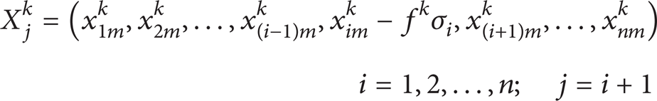
where σ_i is the standard deviation of the ith variable, f is the arbitrary factor, and the initial value range is (1, 3). The computational formula is as follows:

f^{k} = {(f^{(k - 1)})}^{(1 / 2)} .

(3)

This formula indicates that the value of f is not less than 1 regardless of the manner of change. This condition ensures that the distance between new sample points is not extremely small.

When the most probable failure point (MPP) has been updated, the center point for the next iteration can be determined through the following linear interpolation:

X_{m}^{k + 1} = X_{m}^{1} + (X_{D}^{k} - X_{m}^{1}) \frac{g (X_{m}^{1})}{g (X_{m}^{1}) - g (X_{D}^{k})},

(4)

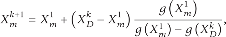
where X_m¹ is the center point in the first iteration, X_D^k is the MPP in the kth iteration, and g(X_m¹) and g(X_D^k) are the response values with respect to X_m^k and X_D^k, respectively.

When the center points are calculated, 2n other sample points are generated by deviating a distance of ± f^{k + 1}σ_i around the center points of the (k + 1)th iteration. The sampling process of the classical RSM given two random variables is shown in Figure 1.

Figure 1:

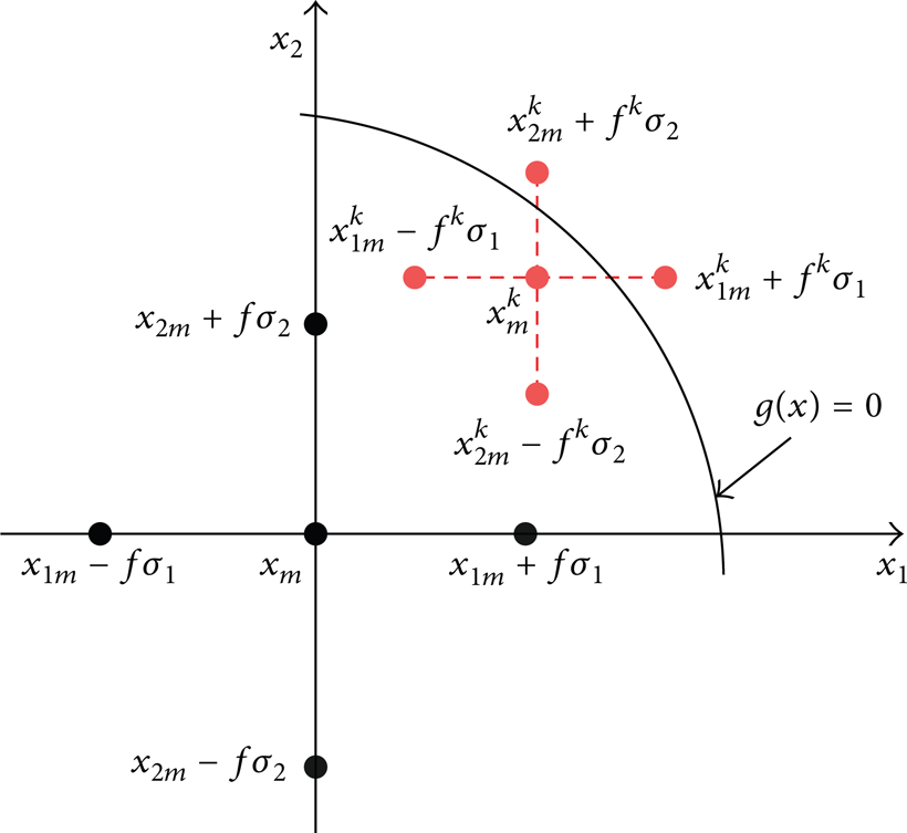
Generation of a new sample point using the classical RSM.

In this figure, x₁ and x₂ are variables, x_m is the initial center point, x_1m^k and x_2m^k are the kth center points of the two variables, f^k is the kth arbitrary factor, and g(x) is the limit state function.

3. ASPIA-Based RSM

The ASPIA-based RSM follows the convergence criterion of the classical RSM, but the manner by which the sample point is produced is significantly improved compared with that of the classical RSM. The flowchart of the ASPIA-based RSM is exhibited in Figure 2.

Figure 2:

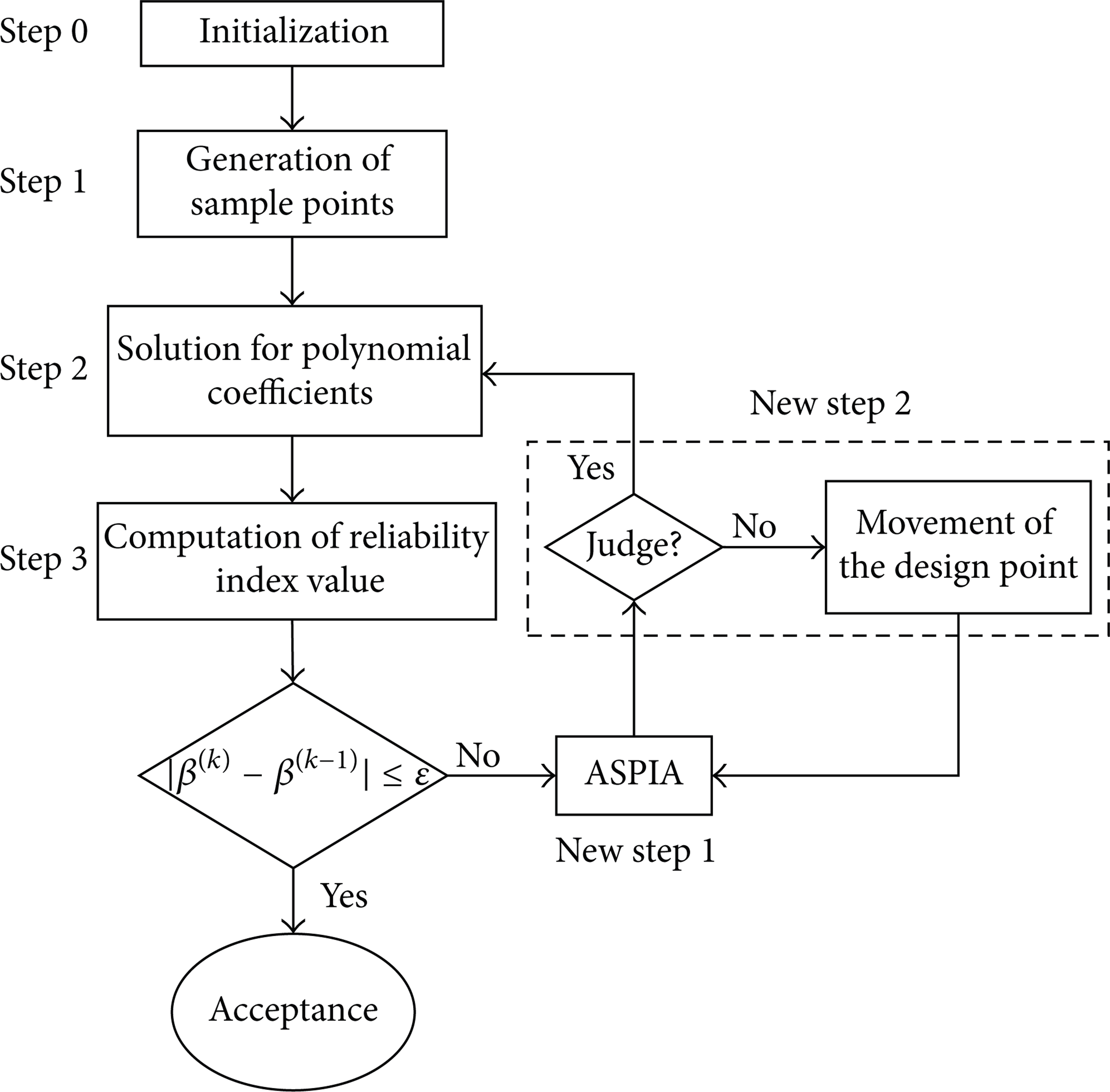
Flowchart of the ASPIA-based RSM.

The difference between the proposed method and classical RSM is the “new step 1” and the “new step 2” depicted in Figure 2. In the classical RSM, these two steps are replaced with the sampling process introduced in Section 2. “New step 1” is the sampling process of the ASPIA-based RSM, whereas “new step 2” includes the judgment on whether the sample points are valid and the mobile MPP strategy applied when the sample points are invalid.

3.1. New Step 1: ASPIA

The purpose of ASPIA is to enable all sample points generated by each iteration to approach the actual limit state. The response surface function can be in the form with or without cross terms. The difference in the response surface function with different forms is that the initial sample points are generated using various approaches. In the iteration process, the sample points are obtained in the same manner by which the linear interpolation of the initial sample points and the current MPP point is performed. The current MPP point is calculated using the first order reliability method (FORM) in the current iteration. The response surface function without cross terms is used to introduce the interpolation process into each iteration and to detail the ASPIA process. This function is written as follows:

\hat{g} (x) = a_{0} + \sum_{i = 1}^{n} b_{i} x_{i} + \sum_{i = 1}^{n} c_{i} x_{i}^{2},

(5)

where n is the number of random variables, x_i is a random variable, and a₀, b_i, and c_i are coefficients.

In (5), 2n + 1 coefficients should be determined. Therefore, at least 2n + 1 samplings are available. Notably, the distributions of random variables are varied and include the uniform, Weibull, and normal distributions. The normal distribution is among the most widely used ones, and other distributions can be converted into it using a certain approach [25, 26]. The most commonly used transformation is given by Rosenblatt [27] as

Φ (u_{i}) = F_{X_{i}} (x_{i}), u_{i} = Φ^{- 1} [F_{X_{i}} (x_{i})],

(6)

where u_i is variable of the standard normal distribution, x_i is original random variable, FX_i(x_i) is the cumulative distribution function (CDF) of x_i, and Φ⁻¹ is the inverse CDF of a standard normal distribution.

Furthermore, the normal distribution is often used to conduct method studies on reliability design, analysis, and optimization [28, 29]. Consequently, the random variables are treated as normal distributions in this study.

The Bucher experimental design is used to generate the initial samples in the response surface function without cross terms. These samples are also the first iteration samples, and they can be denoted as

X^{1} = {[X_{1}^{1}, X_{2}^{1}, X_{3}^{1}, \dots, X_{2 n + 1}^{1}]}^{T},

(7)

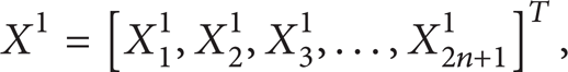
where

\begin{matrix} X_{1}^{1} = X_{m}^{1} = (x_{1 m}^{1}, x_{2 m}^{1}, \dots, x_{n m}^{1}) \\ X_{j}^{1} = (x_{1 m}^{1}, x_{2 m}^{1}, \dots, x_{(i - 1) m}^{1}, x_{i m}^{1} - f^{1} σ_{i}, x_{(i + 1) m}^{1}, \dots, x_{n m}^{1}) \\ i = 1,2, \dots, n; j = i + 1 \\ X_{j}^{1} = (x_{1 m}^{1}, x_{2 m}^{1}, \dots, x_{(i - 1) m}^{1}, x_{i m}^{1} + f^{1} σ_{i}, x_{(i + 1) m}^{1}, \dots, x_{n m}^{1}) \\ i = 1,2, \dots, n; j = n + i + 1 . \end{matrix}

(8)

X_j¹ is the vector of the jth group of sample points generated through Bucher experimental design. Among them, X₁¹ is the center sample point composed of the mean values of random variables.

The response values of the state function at the sample points are represented as follows:

g (X^{1}) = [g (X_{1}^{1}), g (X_{2}^{1}), \dots, g (X_{2 n + 1}^{1})] .

(9)

The kth iteration is also taken as an example. The MPP is still X_D^k, and the response value is g(X_D^k). The value of X_j^{k + 1} that corresponds to g(X_j^{k + 1}) = 0 is obtained through a linear interpolation of [X_j¹, g(X_j¹)] and [X_D^k, g(X_D^k)]. All of the sample points in the (k + 1)th iteration are calculated by

X_{j}^{k + 1} = X_{j}^{1} + (X_{D}^{k} - X_{j}^{1}) \frac{g (X_{j}^{1})}{g (X_{j}^{1}) - g (X_{D}^{k})},

(10)

where X₁^{k + 1} is the center sample point of the (k + 1)th iteration.

The generation of sample points by the proposed method given two random variables is illustrated in Figure 3.

Figure 3:

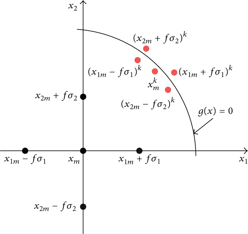
Sample point generation of ASPIA.

In this figure, (x_2m − fσ₂)^k is denoted by the sample point in the kth iteration, which is determined through the linear interpolation of the x_2m − fσ₂ and the MPP obtained in the (k − 1)th iteration. Based on (10) and Figure 3, the proposed method brings not only the center sample points but also other sample points close to the response surface function during each iteration. In addition, this function gradually approaches the actual limit state equation with the increase in the number of iterations. Therefore, the proposed method can bring all of the sample points near the actual limit state equation.

When the response surface function contains cross terms, additional unknown coefficients should be determined. The response surface function with cross terms is expressed as follows:

\hat{g} (x) = a_{0} + \sum_{i = 1}^{n} b_{i} x_{i} + \sum_{i = 1}^{n} c_{i} x_{i}^{2} + \sum_{i = 1}^{n} \sum_{j = i + 1}^{n} d_{i j} x_{i} x_{j} .

(11)

This function has (n + 2)(n + 1)/2 coefficients to be determined, so it requires more samples. The central composite design can be used in this case to generate the initial samples. A total of 2ⁿ + 2n + 1 samples are generated. The sample generation approach in the kth iteration process is identical to that of the response surface function without cross terms.

3.2. New Step 2: Screening of New Sample Points

Although the ASPIA ensures that all of the new sample points are near the actual limit state equation, this method may induce the concentration of the new sample points. The proposed approach to produce other new sample points does not require the arbitrary factor f except in the first iteration. As previously discussed, the value of f is not less than 1, which ensures that the distance between the new sample points is not too small. If this value is unused, the new sample points may concentrate. Thus, two subjects are introduced in this section, namely, the judgment of the distance between the new sample points and the reproduction of these points.

3.2.1. Judgment

If the sample points are too close to one another, the response surface function becomes ill-posed. Thus, the result is erroneous or may even be unsolved. Therefore, the validity of the sample points generated in each iteration must be judged.

When the samples for the response surface function without cross terms are obtained in the kth iteration, the design matrix of (5) is

D = [\begin{bmatrix} 1 & x_{11} & x_{12} & \dots & x_{1 n} & x_{11}^{2} & x_{12}^{2} & \dots & x_{1 n}^{2} \\ 1 & x_{21} & x_{22} & \dots & x_{2 n} & x_{21}^{2} & x_{22}^{2} & \dots & x_{2 n}^{2} \\ ⋮ & ⋮ & ⋮ & ⋮ & ⋮ & ⋮ & ⋮ & ⋮ & ⋮ \\ 1 & x_{q 1} & x_{q 2} & \dots & x_{q n} & x_{q 1}^{2} & x_{q 2}^{2} & \dots & x_{q n}^{2} \end{bmatrix}],

(12)

where the subscript q is the number of samples obtained using the Bucher experimental design q = 2n + 1. The subscript n is the number of random variables and g_i is the sample response value of the ith sample.

The design matrix D in (12) is a square matrix. To judge the validity of the sample points, judgment matrix A can be defined directly by the design matrix D; that is, A = D. However, the design matrix D of (11) for the response surface function with cross terms is not square. The design matrix of (11) is

D = [\begin{bmatrix} 1 & x_{11} & x_{12} & \dots & x_{1 n} & x_{11}^{2} & x_{12}^{2} & \dots & x_{1 n}^{2} & x_{11} x_{12} & x_{11} x_{13} & \dots & x_{1 (n - 1)} x_{1 n} \\ 1 & x_{21} & x_{22} & \dots & x_{2 n} & x_{21}^{2} & x_{22}^{2} & \dots & x_{2 n}^{2} & x_{21} x_{22} & x_{21} x_{23} & \dots & x_{2 (n - 1)} x_{2 n} \\ ⋮ & ⋮ & ⋮ & ⋮ & ⋮ & ⋮ & ⋮ & ⋮ & ⋮ & ⋮ & ⋮ & ⋮ & ⋮ \\ 1 & x_{q 1} & x_{q 2} & \dots & x_{q n} & x_{q 1}^{2} & x_{q 2}^{2} & \dots & x_{q n}^{2} & x_{q 1} x_{q 2} & x_{q 1} x_{q 3} & \dots & x_{q (n - 1)} x_{q n} \end{bmatrix}],

(13)

where the subscript q is the number of samples obtained given the central composite design q = 2ⁿ + 2n + 1. In this case, the judgment matrix A can be defined by

A = D^{T} D .

(14)

Judging the validity of the sample points is similar to judging whether judgment matrix A is ill-conditioned or not. Many methods are used for this purpose [30, 31]. Among them, the condition number is an important judgment method and is expressed by

Cond (A) = ‖A‖ ‖A^{- 1}‖,

(15)

where |·| is denoted by the arbitrary norm and A⁻¹ is the inverse matrix of A.

When the condition number is large, the matrix can be viewed as ill-conditioned. However, the specific value of the condition number that can be used to judge the ill condition of the matrix is difficult to determine. Thus, the method reported in [32] is employed in this study to perform the judgment process as follows:

|\det (A)| \leq 0.01,

(16)

where det stands for the determinant and |·| is the absolute value.

When the determinant of the judgment matrix satisfies (16), the sample points generated are invalid. Therefore, new sample points should be regenerated.

3.2.2. Mobile MPP Strategy

When a new sample point is invalid, the interpolation results of the new sample points are too dense. To address this situation, we propose a mobile MPP strategy that moves the MPP by a certain distance to the vicinity of the curve of the response surface function. This function is obtained in step 2 of the current iteration. We determine the distance by solving the reliability index using the iterative method of FORM [33]. The iterative process is reversed, and the control coefficient λ is introduced to ensure that the process does not deviate excessively from the response surface function. The detailed computation process is as follows.

The kth iteration is taken as an example, and the moving MPP with i times is denoted by X_(i)D^k = (x_(i)D1^k, x_(i)D2^k, …, x_(i)Dn^k). The reliability index that corresponds to MPP is denoted by β_(i)D^k. Moreover, the jth element of this MPP can be obtained as follows using the mobile MPP strategy:

x_{(i) D j}^{k} = x_{(0) D j}^{k} - λ β_{(i - 1) D j}^{k} α_{(i - 1) j}^{k} σ_{j},

(17)

where λ is the control coefficient and the value range is (0, 1). The value of the reliability index β_{(i − 1)Dj}^k and the coefficient α_{(i − 1)j}^k are computed with the following:

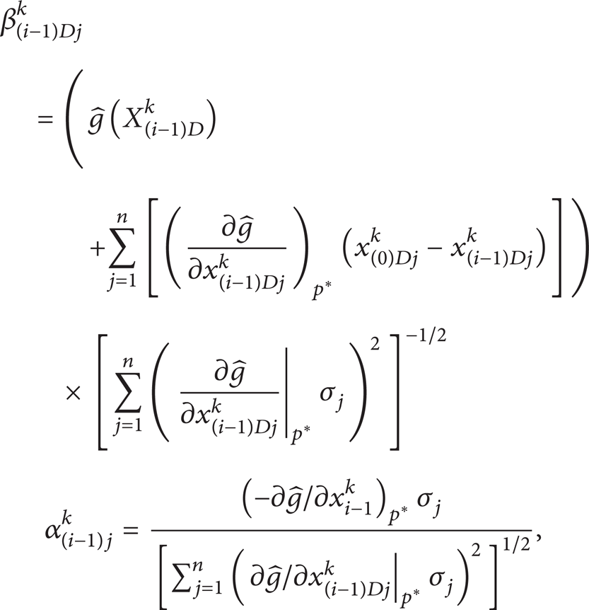
\begin{matrix} β_{(i - 1) D j}^{k} = (\hat{g} (X_{(i - 1) D}^{k})) (+ \sum_{j = 1}^{n} [{(\frac{\partial \hat{g}}{\partial x_{(i - 1) D j}^{k}})}_{p^{*}} (x_{(0) D j}^{k} - x_{(i - 1) D j}^{k})]) \times {([\sum_{j = 1}^{n} {({(\frac{\partial \hat{g}}{\partial x_{(i - 1) D j}^{k}}|}_{p^{*}} σ_{j})}^{2})]}^{- 1 / 2} \\ α_{(i - 1) j}^{k} = \frac{{(- \partial \hat{g} / \partial x_{i - 1}^{k})}_{p^{*}} σ_{j}}{{([\sum_{j = 1}^{n} {({(\partial \hat{g} / \partial x_{(i - 1) D j}^{k}|}_{p^{*}} σ_{j})}^{2})]}^{1 / 2}}, \end{matrix}

(18)

where $\hat{g}$ is the response surface function, σ_j is the standard deviation of x_j, and p* stands for the current MPP X_{(i − 1)D}^k.

When the new MPP X_(i)D^k is obtained, a new set of sample points is generated using (10) until the new samples satisfy the judgment condition. Notably, the center point is excluded from this process.

The mobile process is the inverse process of FORM. The values of (18) can be obtained by solving the reliability index with FORM in each iteration. Meanwhile, (15) and (16) show that the judgment process does not involve calls to the limit state function. Thus, the invalid sampling points cannot increase the number of calls to the limit state function.

4. Numerical Examples and Discussion

In this section, two numerical examples are employed to test the proposed method. Both examples were obtained from [34]. FORM is applied to solve the reliability index under the response surface function with and without cross terms.

4.1. Numerical Example 1

The actual limit state equation is

g (X) = 7 + x_{1} + x_{2} + x_{3} - x_{2}^{3} + x_{3}^{3} - x_{1} x_{2} + x_{1} x_{3},

(19)

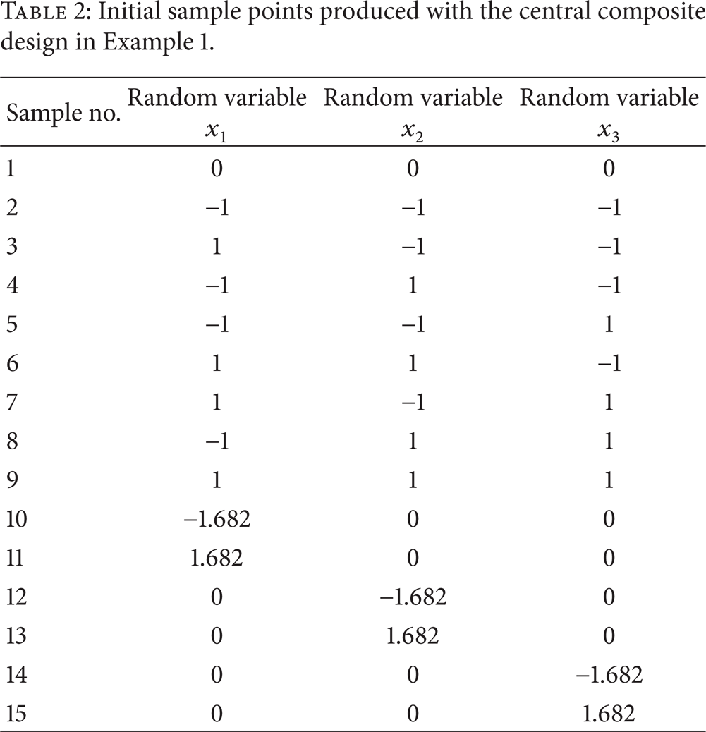
where the random variables are all standard normal distributions. This example is solved given both the response surface function with cross terms and that without. The initial sample points obtained with the Bucher experimental and the central composite designs are listed in Tables 1 and 2, respectively.

Table 1:

Initial sample points determined with the Bucher experimental design in Example 1.

Sampleno.	Random variable x₁	Random variable x₂	Random variable x₃

1	0	0	0
2	−3	0	0
3	0	−3	0
4	0	0	−3
5	3	0	0
6	0	3	0
7	0	0	3

Table 2:

Initial sample points produced with the central composite design in Example 1.

Sample no.	Random variable x₁	Random variable x₂	Random variable x₃

1	0	0	0
2	−1	−1	−1
3	1	−1	−1
4	−1	1	−1
5	−1	−1	1
6	1	1	−1
7	1	−1	1
8	−1	1	1
9	1	1	1
10	−1.682	0	0
11	1.682	0	0
12	0	−1.682	0
13	0	1.682	0
14	0	0	−1.682
15	0	0	1.682

The results obtained by applying the different methods are shown in Table 3.

Table 3:

Calculation results of the different methods applied in Example 1.

Method	MPPs	Reliability index β	Relative error E_β	N ₁ ^a	N ₂ ^b

MCs	—	2.038	0	10⁶	10⁶
Classical RSM	(−0.8567, −1.7173, −0.0335)	1.9195	5.81%	5	35
ASPIA without cross terms	(−0.8726, −1.7096, −0.0523)	1.9201	5.79%	4	28
ASPIA with cross terms	(−0.8726, −1.7095, −0.0356)	1.9257	5.51%	3	45

Number of iterations.

Number of function evaluations.

In the first iteration, the initial samples are applied to fit the response surface function and do not require the judgment process. When the response surface function is utilized with or without cross terms, the number of mobility in each iteration except for the first is 1. For instance, the sample points before and after movement are listed in Table 4 when the response surface function without cross terms is used in the second iteration.

Table 4:

Sample points before and after movement in the second iteration of Example 1.

Before movement			After movement
x ₁	x ₂	x ₃	x ₁	x ₂	x ₃

−0.3644	−1.8813	−0.1906	−0.3644	−1.8813	−0.1906
−0.8162	−1.7532	−0.1776	1.1750	−2.6560	−0.2627
−0.4756	−1.9214	−0.2487	−0.2555	−1.9901	−0.1305
−0.3815	−1.9699	−0.3643	−0.3702	−1.9109	0.1850
−0.1646	−1.9380	−0.1963	−0.8897	−1.9852	−0.1964
−0.2300	0.1037	−0.1203	0.7462	13.6522	0.3810
−0.3883	−2.0047	−0.0883	−0.3562	−1.8385	−0.4281

The judgment condition before movement is ∣det(A)∣ = 9.881 × 10⁻⁹, whereas that after movement is ∣det(A)∣ = 4.746, which satisfies (16).

The judgment condition before movement is |det ⁡ (A)| = 9.881 × 10⁻⁹, whereas that after movement is |det ⁡ (A)| = 4.746, which satisfies (16).

4.2. Numerical Example 2

The limit state equation is as follows:

g (X) = \exp (0.2 x_{1} + 1.4) - x_{2},

(20)

where the random variables are all standard normal distributions. This example is calculated using the response surface function without cross terms. The initial sample points obtained using the Bucher experimental design are presented in Table 5.

Table 5:

Initial sample points obtained using the Bucher experimental design in Example 2.

Sample no.	Random variable x₁	Random variable x₂

1	0	0
2	−3	0
3	0	−3
4	3	0
5	0	3

The results obtained by applying the different methods are depicted in Table 6.

Table 6:

Calculation results of the different methods used in Example 2.

Method	MPP	Reliability index β	Relative error E_β	N ₁ ^a	N ₂ ^b

MCs	—	3.3834	0	10⁶	10⁶
Classical RSM	(−1.7089, 2.8808)	3.3499	0.99%	5	25
ASPIA without cross terms	(−1.709, 2.8811)	3.3546	0.85%	3	15

Number of iterations.

Number of function evaluations.

The number of mobility in each iteration except for the first is 1. The sample points before and after movement in the second iteration are listed in Table 7.

Table 7:

Sample points before and after movement in the second iteration of Example 2.

Before movement		After movement
x ₁	x ₂	x ₁	x ₂

−1.6453	2.9168	−1.6453	2.9168
−1.6225	2.9309	4.8466	6.7443
−1.6407	2.9200	−1.1887	3.1681
−1.6518	2.9083	−2.1753	2.1269
−1.6652	2.9030	3.7498	6.8538
−1.6453	2.9168	−1.6453	2.9168
−1.6225	2.9309	4.8466	6.7443

The judgment condition before movement is ∣det(A)∣ = 4.29 × 10⁻²⁵, whereas that after movement is ∣det(A)∣ = 3.11 × 10³, which satisfies (16).

The judgment condition before movement is |det ⁡ (A)| = 4.29 × 10⁻²⁵, whereas that after movement is |det ⁡ (A)| = 3.11 × 10³, which satisfies (16).

4.3. Discussion

The aforementioned examples indicate that the proposed method has high computational efficiency and an acceptable accuracy in approximating high-order systems that adopt RSM. In practical engineering, the computational result by MCs is typically viewed as the one closest to the actual computational value. Thus, MCs are typically used to verify the results generated with other methods [35], and its computational result is adopted as the standard. Tables 3 and 5 show that the accuracy of the reliability solution for the proposed method is higher than that for the classical RSM. However, the gap is small. Nonetheless, the proposed method is significantly better than the classical method in terms of computational efficiency. In numerical Example 1, 35 function evaluations apply the classical RSM. When the proposed method is used, the number of function evaluations is only 28 for the situation without cross terms and 45 for the situation with cross terms. In numerical Example 2, a total of 25 function evaluations are performed using the classical RSM, whereas only 15 are conducted with the proposed method without cross terms. Function evaluation represents the process of solving function response values; each iteration requires 2n + 1 function evaluations in the condition without cross terms, n is the number of random variables. However, it requires 2ⁿ + 2n + 1 function evaluations for each iteration in the situation with cross terms when the initial sample points are obtained using the central composite design. The use of the response surface function with cross terms results in extensive time cost, but the result accuracy cannot be significantly improved. Hence, the response surface function without cross terms is often employed to solve reliability problems. In practical engineering application, function evaluation is performed by ANSYS. The required calculation cost of this process is high; therefore, reducing the number of function evaluations can effectively improve computational efficiency.

5. Engineering Application

The working cylinder in forging equipment is the final performing element in the forging press. The reliability of this cylinder directly affects work safety performance. Thus, the working cylinder of a 22 MN forging hydraulic press is selected as an engineering example.

The structure diagram of the working cylinder is shown in Figure 4. The random parameters of this cylinder, the mean point, and the standard deviation of each parameter can be determined based on the design. The design parameters of this cylinder are listed in Table 8.

Table 8:

Design parameters and distribution.

Designparameter	Distribution type	Meanvalue	Standarddeviation

D₂/mm	Normal distribution	1230	4
D₃/mm	Normal distribution	1200	4
D₄/mm	Normal distribution	1210	4
D₅/mm	Normal distribution	1200	4
D₆/mm	Normal distribution	256	3
D₇/mm	Normal distribution	240	3
D₈/mm	Normal distribution	820	3
L₂/mm	Normal distribution	500	3
L₃/mm	Normal distribution	1680	4
L₄/mm	Normal distribution	400	3
L₅/mm	Normal distribution	300	3
L₆/mm	Normal distribution	10	2
P/MPa	Normal distribution	60	12
S/MPa	Normal distribution	300	22

Figure 4:

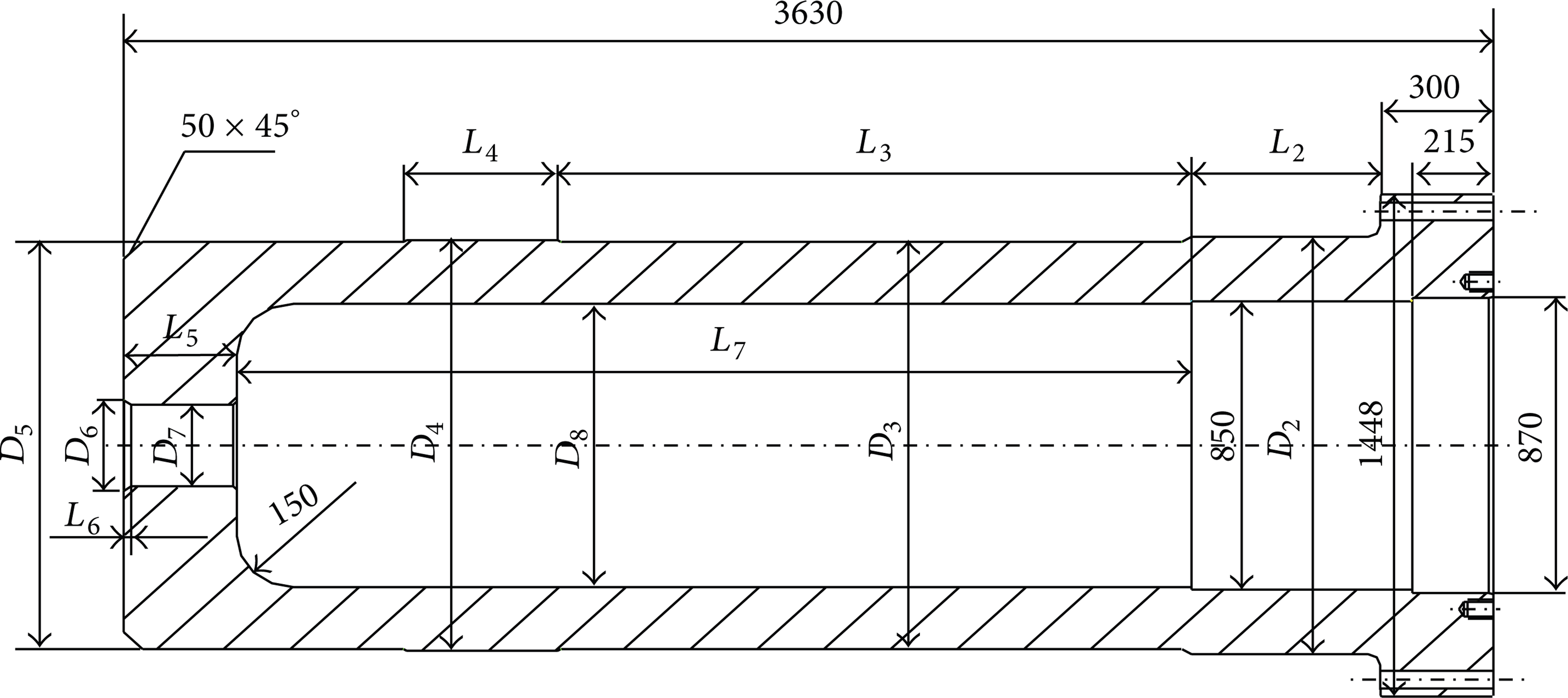
Structural diagram of the working cylinder.

In Figure 4 and Table 8, D_i is the diameter of relevant position, L_i is the length of relevant position, P is the pressure of the working cylinder, and S is the yield strength of material.

MATLAB and ANSYS software are combined in this study to solve the function response value of the working cylinder. The 3D parametric model of this cylinder is established using the parametric design language of ANSYS [36]. The 1/4 finite model of the working cylinder is constructed according to its structure and loads. The applied loads and constraints are also depicted in Figure 5, which can be specifically described as follows.

The symmetry constraint (SYMM) is applied on the separating surface of the 1/4 finite model.

The displacement constraint of the X direction (UX) is applied on the left surface.

The rotational restraint of the X axis (ROTX) is applied on the cylindrical surface of D₂.

Pressure load (PRES) is applied within the working cylinder, which is the surface of the inner hole of D₇, D₈, and the connection part.

Figure 5:

Loads and constraints applied to the working cylinder.

The stress contour of the working cylinder is displayed in Figure 6. The dangerous part is located in the inner wall.

Figure 6:

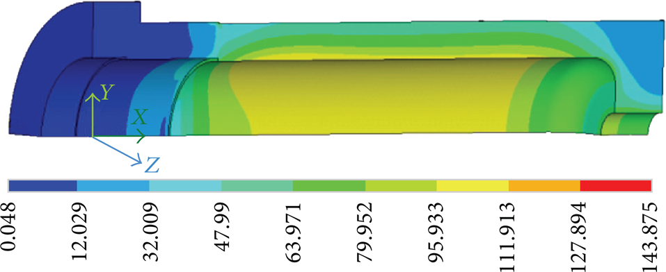
Stress contour of the working cylinder.

MATLAB is used to obtain the numerical values of each ASPIA design variable. ANSYS is then activated by the “system” statement of MATLAB, and maximum stress is determined using ANSYS. The value of yield strength S minus maximum stress is the response value that corresponds to the design variables in this iteration. Finally, the response value is returned through the “load” statement of MATLAB. The quadratic equation for the current data is fitted by MATLAB. The limit state equation of the working cylinder is eventually solved through repeated iterations as follows:

\begin{matrix} g (X) = 196.36 {D_{2}}^{2} - 4.83 \times 1 0^{5} D_{2} + 197.53 {D_{3}}^{2} - 4.74 \times 1 0^{5} D_{3} \\ + 1149.12 {D_{4}}^{2} - 2.78 \times 1 0^{6} D_{4} + 251.18 {D_{5}}^{2} - 6.03 \times 1 0^{5} D_{5} \\ + 697.60 {D_{6}}^{2} - 3.57 \times 1 0^{5} D_{6} + 570.40 {D_{7}}^{2} - 2.74 \times 1 0^{5} D_{7} \\ - 780.95 \times {D_{8}}^{2} + 1.28 \times 1 0^{6} D_{8} - 1598.02 {L_{2}}^{2} + 1.60 \times 1 0^{6} L_{2} \\ + 324.65 {L_{3}}^{2} - 1.09 \times 1 0^{6} L_{3} + 248.69 {L_{4}}^{2} - 1.99 \times 1 0^{5} L_{4} \\ - 932.03 {L_{5}}^{2} + 5.59 \times 1 0^{5} L_{5} + 366.12 {L_{6}}^{2} - 7.33 \times 1 0^{3} L_{6} \\ + 6.74 \times 1 0^{4} P^{2} - 1.05 \times 1 0^{7} P - 5.10 \times 1 0^{3} S^{2} \\ + 2.89 \times 1 0^{6} S + 2.65 \times 1 0^{9} . \end{matrix}

(21)

The value of reliability index β is 1.684 and that of the corresponding reliability is 0.9549. The reliability of the working cylinder is analyzed using the ANSYS MCs method, and the reliability value is 0.9774 after 10⁶ simulation cycles. In addition, the reliability error attributed to the proposed and the MCs methods is only 2.25%. Based on the fitting function, the coefficients of pressure P and yield strength S are large. This result suggests that the two variables strongly affect the reliability of the working cylinder in accordance with the actual situation.

6. Conclusions

This paper proposes a new RSM based on ASPIA. Unlike the classical RSM, the ASPIA-based RSM can not only quickly bring all sample points close to the actual limit state equation but also ensure the precision of the reliability solution. Meanwhile, the concentration problem of sample points during the ASPIA process is resolved using the mobile MPP strategy. This strategy utilizes the judgment criterion of point distance and the moving MPP. Two numerical examples are used to successfully test the proposed method, and the results indicate that the proposed method has high computational efficiency. At the same time, the use of the response surface function with cross terms results in extensive time cost. However, result accuracy cannot be improved considerably. Therefore, the response surface function without cross terms is often employed to solve reliability problems in practical engineering. Finally, the proposed method is applied to analyze the reliability of the working cylinder of a 22 MN forging hydraulic press. This analysis combines MATLAB and ANSYS software. The dangerous part of the working cylinder is located in the inner wall, and the changes in pressure P and yield strength S strongly affect its reliability.

Conflict of Interests

The authors declare that there is no conflict of interests regarding the publication of this paper.

Footnotes

Acknowledgments

The authors gratefully acknowledge the funding support from the National Natural Science Foundation of China (Grant no. 51175019) and the National Key Technology R&D Program, China (Grant no. 2015BAF04B00). They thank the anonymous reviewers for their valuable comments.

References

Gaspar

and Soares

C. G.

, “Hull girder reliability using a Monte Carlo based simulation method,” Probabilistic Engineering Mechanics, vol. 31, pp. 65–75, 2013.

Janssen

, “Monte-Carlo based uncertainty analysis: sampling efficiency and sampling convergence,” Reliability Engineering and System Safety, vol. 109, pp. 123–132, 2013.

Bordas

S. P. A.

Natarajan

Kerfriden

, “On the performance of strain smoothing for quadratic and enriched finite element approximations (XFEM/GFEM/PUFEM),” International Journal for Numerical Methods in Engineering, vol. 86, no. 4–5, pp. 637–666, 2011.

Ryckelynck

Benziane

D. M.

Musienko

, and Cailletaud

, “Toward “green” mechanical simulations in materials science: hyper-reduction of a polycrystal plasticity model,” European Journal of Computational Mechanics, vol. 19, no. 4, pp. 365–388, 2010.

Kerfriden

Passieux

J. C.

, and Bordas

S. P.

, “Local/global model order reduction strategy for the simulation of quasi-brittle fracture,” International Journal for Numerical Methods in Engineering, vol. 89, no. 2, pp. 154–179, 2012.

Chamoin

Oden

J. T.

, and Prudhomme

, “A stochastic coupling method for atomic-to-continuum Monte-Carlo simulations,” Computer Methods in Applied Mechanics and Engineering, vol. 197, no. 43–44, pp. 3530–3546, 2008.

Ryckelynck

Vincent

, and Cantournet

, “Multidimensional a priori hyper-reduction of mechanical models involving internal variables,” Computer Methods in Applied Mechanics and Engineering, vol. 225–228, pp. 28–43, 2012.

Bucher

C. G.

and Bourgund

, “A fast and efficient response surface approach for structural reliability problems,” Structural Safety, vol. 7, no. 1, pp. 57–66, 1990.

Rajashekhar

M. R.

and Ellingwood

B. R.

, “A new look at the response surface approach for reliability analysis,” Structural Safety, vol. 12, no. 3, pp. 205–220, 1993.

10.

Kimand

S.-H.

S.-W.

, “Response surface method using vector projected sampling points,” Structural Safety, vol. 19, no. 1, pp. 3–19, 1997.

11.

Das

P. K.

and Zheng

, “Cumulative formation of response surface and its use in reliability analysis,” Probabilistic Engineering Mechanics, vol. 15, no. 4, pp. 309–315, 2000.

12.

Das

P. K.

, and Zheng

, “Stepwise response surface method and its application in reliability analysis of ship hull structure,” Journal of Offshore Mechanics and Arctic Engineering, vol. 124, no. 4, pp. 226–230, 2002.

13.

Kaymaz

and McMahon

C. A.

, “A response surface method based on weighted regression for structural reliability analysis,” Probabilistic Engineering Mechanics, vol. 20, no. 1, pp. 11–17, 2005.

14.

Nguyen

X. S.

Sellier

Duprat

, and Pons

, “Adaptive response surface method based on a double weighted regression technique,” Probabilistic Engineering Mechanics, vol. 24, no. 2, pp. 135–143, 2009.

15.

Allaix

D. L.

and Carbone

V. I.

, “An improvement of the response surface method,” Structural Safety, vol. 33, no. 2, pp. 165–172, 2011.

16.

Liu

and Li

, “An improved adaptive response surface method for structural reliability analysis,” Journal of Central South University of Technology, vol. 19, no. 4, pp. 1148–1154, 2012.

17.

Roussouly

Petitjean

, and Salaun

, “A new adaptive response surface method for reliability analysis,” Probabilistic Engineering Mechanics, vol. 32, pp. 103–115, 2013.

18.

Tsai

Y.-T.

and Wang

K.-S.

, “A study of sample size analysis to support reliability test programming,” Journal of the Chinese Society of Mechanical Engineers, vol. 28, no. 3, pp. 315–323, 2007.

19.

Cho

I.-H.

and Zoh

K.-D.

, “Photocatalytic degradation of azo dye (Reactive Red 120) in TiO₂/UV system: optimization and modeling using a response surface methodology (RSM) based on the central composite design,” Dyes and Pigments, vol. 75, no. 3, pp. 533–543, 2007.

20.

Cheng

and Li

Q. S.

, “Application of the response surface methods to solve inverse reliability problems with implicit response functions,” Computational Mechanics, vol. 43, no. 4, pp. 451–459, 2009.

21.

Luo

, “Optimization of total polysaccharide extraction from Dioscorea nipponica Makino using response surface methodology and uniform design,” Carbohydrate Polymers, vol. 90, no. 1, pp. 284–288, 2012.

22.

Lü

Z.-Z.

Zhao

, and Yue

Z.-F.

, “Advanced response surface method for mechanical reliability analysis,” Applied Mathematics and Mechanics, vol. 28, no. 1, pp. 19–26, 2007.

23.

Wong

S. M.

Hobbs

R. E.

, and Onof

, “An adaptive response surface method for reliability analysis of structures with multiple loading sequences,” Structural Safety, vol. 27, no. 4, pp. 287–308, 2005.

24.

Yan

Sun

, and Yang

, “Analysis method of reliability sensitivity based on response surface methods,” Chinese Journal of Mechanical Engineering, vol. 43, no. 10, pp. 67–71, 2007.

25.

and Chen

, “Collaborative reliability analysis under the framework of multidisciplinary systems design,” Optimization and Engineering, vol. 6, no. 1, pp. 63–84, 2005.

26.

Jiang

W. X.

Han

Liu

L. X.

, and Le

P. H.

, “Structural reliability analysis based on random distributions with interval parameters,” Computers and Structures, vol. 89, no. 23–24, pp. 2292–2302, 2011.

27.

Rosenblatt

, “Remarks on a multivariate transformation,” Annals of Mathematical Statistics, vol. 23, pp. 470–472, 1952.

28.

, “Unified uncertainty analysis by the first order reliability method,” Journal of Mechanical Design, vol. 130, no. 9, Article ID 091401, 10 pages, 2008.

29.

Huang

H.-Z.

Zhang

Zeng

, and Wang

, “Collaborative optimization with inverse reliability for multidisciplinary systems uncertainty analysis,” Engineering Optimization, vol. 42, no. 8, pp. 763–773, 2010.

30.

Choi

H. G.

Thite

A. N.

, and Thompson

D. J.

, “A threshold for the use of Tikhonov regularization in inverse force determination,” Applied Acoustics, vol. 67, no. 7, pp. 700–719, 2006.

31.

Wang

Law

S. S.

, and Yang

Q. S.

, “Sensor placement methods for an improved force identification in state space,” Mechanical Systems and Signal Processing, vol. 41, no. 1–2, pp. 254–267, 2013.

32.

H. D.

, “Ill-conditioned Matrix and Its Improvement in Regression,” Acta Agronomica Sinica in Chinese Journal, vol. 32, no. 1, pp. 1–6, 2006.

33.

X. P.

and Sudjianto

, “First-order saddle point approximation for reliability analysis,” American Institute of Aeronautics and Astronautics Journal, vol. 42, no. 6, pp. 1199–1207, 2004.

34.

Zheng

and Das

P. K.

, “Improved response surface method and its application to stiffened plate reliability analysis,” Engineering Structures, vol. 22, no. 5, pp. 544–551, 2000.

35.

Rahbari

N. Mohajer

Talatahari

, and Aalami

, “Reliability analysis of semiactive magnetorheological dampers subjected to harmonic excitations,” Advances in Mechanical Engineering, vol. 2013, Article ID 643927, 7 pages, 2013.

36.

Zhang

L. X.

Liu

S. R.

Mao

E. R.

, “Reliability analysis of agricultural machinery chassis drive axle housing based on ANSYS,” Transactions of the Chinese Society of Agricultural Engineering, vol. 27, no. 2, pp. 37–44, 2013.

A New Sampling Approach for Response Surface Method Based Reliability Analysis and Its Application

Abstract

1. Introduction

2. Sampling of Classical RSM

3. ASPIA-Based RSM

3.1. New Step 1: ASPIA

3.2. New Step 2: Screening of New Sample Points

3.2.1. Judgment

3.2.2. Mobile MPP Strategy

4. Numerical Examples and Discussion

4.1. Numerical Example 1

4.2. Numerical Example 2

4.3. Discussion

5. Engineering Application

6. Conclusions

Conflict of Interests

Footnotes

Acknowledgments

References