Corrected Statistical Energy Analysis Model for Car Interior Noise

Abstract

Statistical energy analysis (SEA) is a well-known method to analyze the flow of acoustic and vibration energy in a complex structure. For an acoustic space where significant absorptive materials are present, direct field component from the sound source dominates the total sound field rather than a reverberant field, where the latter becomes the basis in constructing the conventional SEA model. Such environment can be found in a car interior and thus a corrected SEA model is proposed here to counter this situation. The model is developed by eliminating the direct field component from the total sound field and only the power after the first reflection is considered. A test car cabin was divided into two subsystems and by using a loudspeaker as a sound source, the power injection method in SEA was employed to obtain the corrected coupling loss factor and the damping loss factor from the corrected SEA model. These parameters were then used to predict the sound pressure level in the interior cabin using the injected input power from the engine. The results show satisfactory agreement with the directly measured SPL.

1. Introduction

The level of noise in a car interior has become an issue since the past decades as a parameter to define a quality of a motor vehicle besides its performance, safety, and the fuel economy [1]. Simulation techniques, as well as measurements, are developed to accurately predict the interior noise level. Among existing prediction methods to calculate the structural vibration and noise energy level inside the cabin are namely, finite element analysis (FEA) and statistical energy analysis (SEA). The FEA can be effectively employed for low frequency range problem where distinct modes in the energy are present. Meanwhile, the SEA is particularly applied for high frequency range, where modes are overlapping and the energy level behaves “statistically,” in which only its average value is of interest. In this case, use of FEA will be too costly as a greater number of numerical elements is required to accurately represent smaller wavelength.

For application in automotive in particular, SEA is usually implemented for predicting the noise level inside a car cabin. DeJong [2] measured three sources of interior noise: the engine, tires, and airflow, and these were used as inputs to the SEA model to predict sound pressure level inside the car cabin. Steel [3] presented the analysis of structural vibration transmission through a motor car using SEA model where the body of the motor car was modelled as a system of connected flat plates for predictive purpose. Marzbanrad and Alahyari [4] studied the acoustic environment in the car cabin under the influence of high frequency aerodynamics sources using SEA method. Some panels on the windshield, the roof, the doors, and the floor of a vehicle were simulated as input sources of noise when the car was moving at high speed. Sound pressure level formulation is presented and is used for comparison with the experimental results. SEA has also been widely used for noise and vibration analysis in aerospace, railway vehicle [5], and building acoustics [6] including an electric motor [7].

In SEA, a system is first breached into several subsystems and the energy flow between subsystems is then calculated. The requirement is that the energy in a subsystem should be dominated with resonant modes (reverberant field). However, this condition is not always found for certain cases in practice, for example, structures consisting of stiff components where use of SEA will not provide accurate prediction. Therefore attempts have also been proposed to modify or to improve the SEA model for these particular cases.

Renji et al. [8] proposed modified SEA formulation for the nonresonant response. The model is similar to the conventional SEA model for resonant response but uses different expression for the CLFs which are based on the sound power transmission and absorption coefficient of the structure. The nonresonant response is not significant for limp panels, but very much significant for thin light panels. Ribeiro and Smith [9] developed a prediction method of the sound field inside large acoustic spaces where it is not possible to assume a uniform reverberant field due to attenuation and scattering. The method separates the direct and reverberant sound field contributions by the SEA framework using a correction to the traditional SEA equation. Lei et al. [10] presented an improved SEA model for predicting structural response and noise reduction of acoustical enclosures in a more broad frequency range, not only at the high frequencies, but also at the low and intermediate frequencies. The prediction accuracy is improved including the resonant and nonresonant responses in entire energy transfer path, although there are not enough resonant modes of structural and acoustical subsystems at the low and intermediate frequencies. More accurate transmission coefficient, which includes the effect of bending stiffness, size of structure and forced radiation efficiency is used to calculate the CLFs between the sound field and finite panels.

Acoustic absorber in a cavity, for example, in vehicle interior cabin is to reduce the sound reflection as well as to reduce sound transmission from the exterior. Condition of a reverberant field will thus not be fulfilled in this system and thus the classical SEA model will give less accurate prediction of the energy level in the interior. Corrected SEA model is therefore required to counter this situation and is the main objective of this paper.

2. Development of the Corrected SEA Model

2.1. Governing Equation

Consider a system divided into N subsystems; each is injected with input power P_in as shown in Figure 1. Some of the power will dissipate through damping and the rest is exchanged among other subsystems through couplings. Based on the power balance principle, the input power P_in at subsystem-i is thus given by [11]

$P_{\text{in},i}=\omega {\eta }_i{E}_i+{\displaystyle \sum }_{\begin{array}{c}j=\mathrm{1}\\ j\ne i\end{array}}^N‍\omega {\eta }_{ij}{E}_i-{\displaystyle \sum }_{\begin{array}{c}j=\mathrm{1}\\ j\ne i\end{array}}^N‍\omega {\eta }_{ji}{E}_j,$

(1)

where ω is the frequency angular, E is the energy, η _i is the damping loss factor at the ith subsystem, and η _ij is the coupling loss factor from the ith to the jth subsystem. The first term on the right hand side of (1) is the dissipation of power P _d in subsystem-i. The second term corresponds to the power flow P _c from subsystem-i to subsystem-j due to coupling and vice versa for the third term.

Figure 1:

A schematic diagram of SEA model.

In an enclosed acoustic space, the total energy of the sound field at any given location is the sum of energy from the direct field E_dir radiated by the sound source and the reverberant field E_rev created by the reflections expressed as

$E=E_{\text{dir}}+E_{\text{rev}}.$

(2)

For a room with highly reflective walls, for example, reverberant chamber, the sound energy at a location (away from the source) in the room can be assumed to come from any possible angles of incidence. The condition is usually called “diffuse” where high modal overlap of acoustic modes exists in a frequency band.

If the walls of the room are treated with absorbent materials, energy from reflections will be reduced and the direct field component dominates the total sound field. For this damped acoustic space, as the SEA model is based on the assumption of reverberant energy, it is therefore important to separate the direct field component from the total energy. Under steady state condition, the power balance equation in (1) can be expressed as

$P_{\text{in},i}\left(\mathrm{1}-{\overline{\alpha }}_i\right)=\omega {\eta }_i{E}_{\text{rev},i}+{\displaystyle \sum }_{\begin{array}{c}j=\mathrm{1}\\ j\ne i\end{array}}^N‍\omega {\eta }_{ij}{E}_{\text{rev},i}-{\displaystyle \sum }_{\begin{array}{c}j=\mathrm{1}\\ j\ne i\end{array}}^N‍\omega {\eta }_{ji}{E}_{\text{rev},j},$

(3)

where $\overline{\alpha }$ is the average absorption coefficient in ith subsystem and E_{rev, i} is the reverberant field component after the removal of the direct field component from the measured signal in the corresponding subsystem. Note that the term $P_{\text{in},i}(\mathrm{1}-{\overline{\alpha }}_i)$ accounts for the loss of the power at the first reflection. It is also important to note that (3) is applied for the case of reduction of the reverberant energy (or the increase of the direct field energy) due to the presence of the absorptive materials inside the acoustic space. However, the transition frequency between the direct field and the reverberant field is also bounded by the dimensions of the room due to the nature of the acoustic modes (or the modal overlap) in the room. This crossover frequency is defined by Schroeder [12] as the function of the room volume and the reverberation time, above which the diffuse field (fully reverberant field) applies.

This corrected SEA model has been used by Ribeiro and Smith [9] to develop a prediction method of the sound field inside large acoustic spaces where it is not possible to assume a uniform reverberant field due to attenuation and scattering. The direct field contribution is determined by assuming spherical propagation away from a point source. From here, the energy from the direct field can be calculated and can therefore be eliminated to leave only the reverberant energy. Another assumption is also made where no obstacles are located between the source and the receiver. However this is difficult to implement especially for a complex environment such as a factory with distributed machineries. The directivity of the source has to also be taken into account to obtain more accurate results.

2.2. Elimination of Direct Field Component from Measured Impulse Response

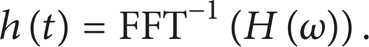
In a small enclosed space such as a car cabin, the assumption of spherical propagation is difficult to hold particularly for a receiver close to the source. A new approach is proposed here to determine the direct field component from the measured signal in corresponding subsystem. The direct field component can be identified from the measured impulse response h(t) where this is obtained by applying inverse fast fourier transform (FFT) to the measured frequency response function (FRF) H(ω) in subsystem

$h\left(t\right)={\text{FFT}}^{-\mathrm{1}}\left(H\left(\omega \right)\right).$

(4)

For a sound field which is not completely reverberant, that is, there is significant energy from direct field contribution, the impulse response features will consist of an initial peak due to the direct field component and be followed by other peaks, that is, the reflected signals building up the reverberant field. This direct field component can thus be removed by applying a simple unit step window function w(t) to the impulse response given by

$w\left(t\right)=\left\{\begin{array}{cc}\mathrm{0},\hfill & \text{for}\hspace{0.17em}\hspace{0.17em}t\le t_a,\hfill \\ \mathrm{1},\hfill & \text{for}\hspace{0.17em}\hspace{0.17em}t>t_a,\hfill \end{array}\right)$

(5)

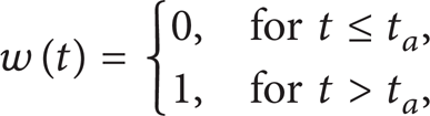
where t _a is the arrival time of the first reflection. The FRF without the direct field component can be obtained by applying back the FFT to the corrected impulse response. The methodology is summarized in Figure 2.

Figure 2:

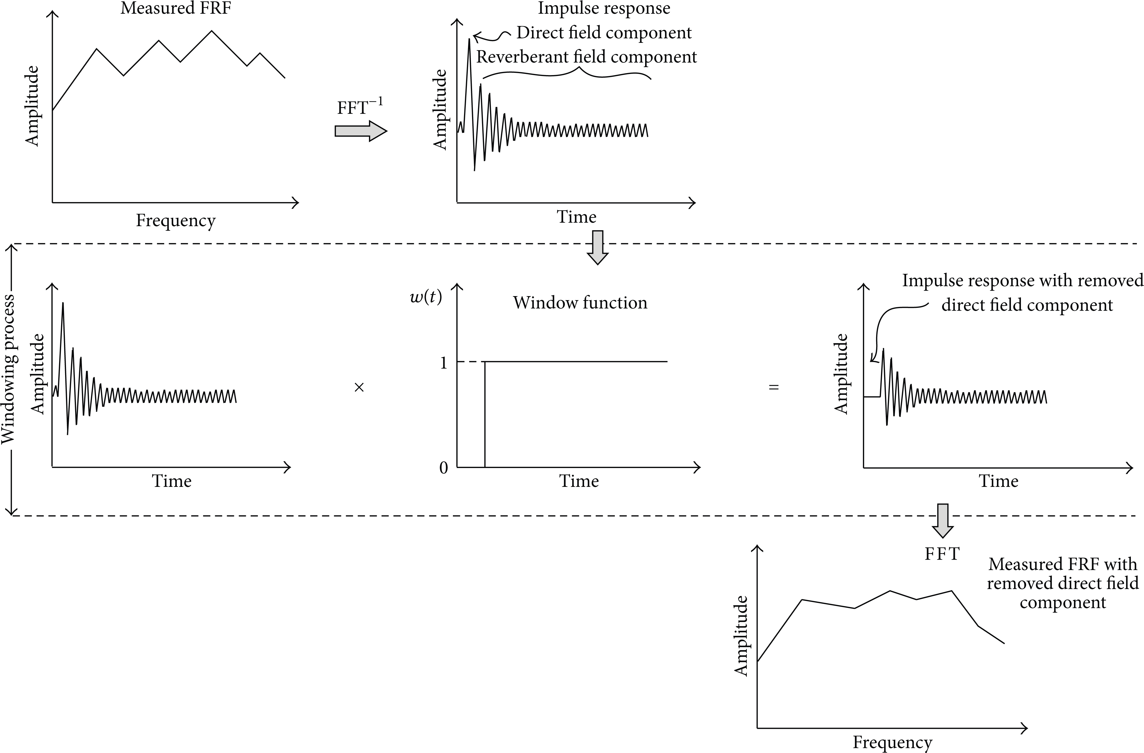
Diagram of methodology to remove the direct field component.

3. Experiment

3.1. Experimental SEA: Power Injection Method

The power injection method is one of techniques used to estimate the SEA parameters, namely, the coupling loss factor (CLF) and the damping loss factor (DLF), through experiment. Suppose there are only two subsystems (refer again to Figure 1); from (1), this can be written in matrix form as

$\left\{\begin{array}{c}{P}_{\text{in},\mathrm{1}}\\ P_{\text{in},\mathrm{2}}\end{array}\right\}=\omega \left[\begin{array}{cc}{\eta }_{\mathrm{1}}+{\eta }_{\mathrm{12}}& -{\eta }_{\mathrm{21}}\\ -{\eta }_{\mathrm{12}}& {\eta }_{\mathrm{2}}+{\eta }_{\mathrm{21}}\end{array}\right]\left\{\begin{array}{c}{E}_{\mathrm{1}}\\ E_{\mathrm{2}}\end{array}\right\}.$

(6)

If only subsystem-1 is excited over some frequency band with measured input power P₁⁽¹⁾ while P₂ = 0, thus

$\left\{\begin{array}{c}{P}_{\mathrm{1}}^{\left(\mathrm{1}\right)}\\ \mathrm{0}\end{array}\right\}=\omega \left[\begin{array}{cc}{\eta }_{\mathrm{1}}+{\eta }_{\mathrm{12}}& -{\eta }_{\mathrm{21}}\\ -{\eta }_{\mathrm{12}}& {\eta }_{\mathrm{2}}+{\eta }_{\mathrm{21}}\end{array}\right]\left\{\begin{array}{c}{E}_{\mathrm{1}}^{\left(\mathrm{1}\right)}\\ E_{\mathrm{2}}^{\left(\mathrm{1}\right)}\end{array}\right\},$

(7)

where E₁⁽¹⁾ and E₂⁽¹⁾ are the measured subsystem energies due to the injected power in subsystem-1. Now the subsystem-2 is excited with input power P₂⁽²⁾; then

$\left\{\begin{array}{c}\mathrm{0}\\ P_{\mathrm{2}}^{\left(\mathrm{2}\right)}\end{array}\right\}=\omega \left[\begin{array}{cc}{\eta }_{\mathrm{1}}+{\eta }_{\mathrm{12}}& -{\eta }_{\mathrm{21}}\\ -{\eta }_{\mathrm{12}}& {\eta }_{\mathrm{2}}+{\eta }_{\mathrm{21}}\end{array}\right]\left\{\begin{array}{c}{E}_{\mathrm{1}}^{\left(\mathrm{2}\right)}\\ E_{\mathrm{2}}^{\left(\mathrm{2}\right)}\end{array}\right\}.$

(8)

Combining (7) and (8) yields

$\left[\begin{array}{cc}{P}_{\mathrm{1}}^{\left(\mathrm{1}\right)}& \mathrm{0}\\ \mathrm{0}& P_{\mathrm{2}}^{\left(\mathrm{2}\right)}\end{array}\right]=\omega \left[\begin{array}{cc}{\eta }_{\mathrm{1}}+{\eta }_{\mathrm{12}}& -{\eta }_{\mathrm{21}}\\ -{\eta }_{\mathrm{12}}& {\eta }_{\mathrm{2}}+{\eta }_{\mathrm{21}}\end{array}\right]\left[\begin{array}{cc}{E}_{\mathrm{1}}^{\left(\mathrm{1}\right)}& E_{\mathrm{1}}^{\left(\mathrm{2}\right)}\\ E_{\mathrm{2}}^{\left(\mathrm{1}\right)}& E_{\mathrm{2}}^{\left(\mathrm{2}\right)}\end{array}\right].$

(9)

The SEA parameters can be therefore calculated as

$\left[\begin{array}{cc}{\eta }_{\mathrm{1}}+{\eta }_{\mathrm{12}}& -{\eta }_{\mathrm{21}}\\ -{\eta }_{\mathrm{12}}& {\eta }_{\mathrm{2}}+{\eta }_{\mathrm{21}}\end{array}\right]=\frac{\mathrm{1}}{\omega }\left[\begin{array}{cc}{P}_{\mathrm{1}}^{\left(\mathrm{1}\right)}& \mathrm{0}\\ \mathrm{0}& P_{\mathrm{2}}^{\left(\mathrm{2}\right)}\end{array}\right]{\left[\begin{array}{cc}{E}_{\mathrm{1}}^{\left(\mathrm{1}\right)}& E_{\mathrm{1}}^{\left(\mathrm{2}\right)}\\ E_{\mathrm{2}}^{\left(\mathrm{1}\right)}& E_{\mathrm{2}}^{\left(\mathrm{2}\right)}\end{array}\right]}^{-\mathrm{1}}.$

(10)

3.2. Methodology

The measurement was conducted in a car cabin where the passenger compartment is divided into two subsystems, that is, the front cabin and the rear cabin, by assuming the front seats as the coupling between the two subsystems. The methodology for this experiment can be divided into two steps. Firstly the loudspeaker was used to inject the sound energy into the subsystems (i.e., at the front and rear cabins). In this stage, the engine of the test vehicle is turned off. Using the classical SEA model, the CLF and DLF with the effect of direct field components are obtained. From here, the impulse response from the cabin was also be obtained. Thus by eliminating the direct field component, the corrected CLF and DLF can be calculated using the corrected SEA model.

Secondly, the engine is now turned on to provide the energy input into the cabin. The sound power from the engine through the bulk head is then measured using sound intensity technique. Using the measured sound power through the classical SEA model, the energy in the cabin in terms of the sound pressure level (SPL) can therefore be obtained, either using the uncorrected CLF and DLF or using the corrected CLF and DLF. The results can then be compared with the SPL directly measured in the car interior. Figure 3 shows the flow chart of the methodology.

Figure 3:

Diagram of methodology for experiment SEA in the car cabin.

As discussed in Section 2.2, in order to obtain the impulse response, the data was recorded as the frequency response function (FRF) between the signal from the source to that from the response point. For this purpose, the reference microphone was located in front of the loudspeaker as seen in Figure 4. Assuming the system is linear, this technique also eliminates the dependency of the results on the amplification of the loudspeaker and to ensure equivalent analysis is made among sets of experiments. The measured FRF is defined as

$H\left(\omega \right)=\frac{S_{xy}\left(\omega \right)}{S_{xx}\left(\omega \right)},$

(11)

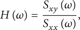
where S _xy is the cross-spectrum between the reference microphone and the response microphone and S _xx is the autospectrum from the reference microphone.

Figure 4:

Location of the sound source and the reference microphone in the front cavity.

3.3. Measurement of Sound Power

The accuracy of the SEA method depends on the accuracy of the input power as shown in (10). A 100 Watt loudspeaker was used as the sound source to inject the sound energy in the car cabin. The sound power measurement from the loudspeaker was therefore conducted according to BS-ISO 3746 [13] in a semianechoic chamber to provide good precision of measurement and good accuracy of results. Two 1/2-inch G.R.A.S acoustic microphones type 40 AE with preamplifier type 26CA were used to record the sound pressure level. Before the measurement, each microphone was calibrated using a G.R.A.S pistonphone calibrator type 42AA. The data was processed through the LDS Photon⁺ signal analyzer and transferred to computer. The experimental setup for the sound power measurement is shown in Figure 5.

Figure 5:

Experimental setup for the sound power measurement inside a semianechoic chamber.

The acoustic pressure was measured over ten measurement locations forming a hemispherical surface enclosing the loudspeaker. The measurement distance between loudspeaker and each of microphone positions is 1 m. The sound power from the loudspeaker was also measured in terms of the FRF as given in (11). The spatial average of the FRF, 〈H(ω)〉, over the hemispherical surface was calculated and the equivalent normalised sound power level is given by

$\widehat{P}\left(\omega \right)=\frac{〈H\left(\omega \right)〉}{\rho c}\times S,$

(12)

where S = 2πr² is the area of the hemispherical surface with r being the distance of the response microphone from the loudspeaker, ρ the air density, and c the speed of sound.

The measured normalised sound power level in one-third octave bands can be seen in Figure 6. It shows that the sound power is almost flat from 500 Hz to 6 kHz, which can provide sufficient injected energy for the whole corresponding frequency bands.

Figure 6:

Measured normalised sound power from the loudspeaker.

The next section presents the estimation of the SEA parameters: the CLF and DLF from the reverberation and nonreverberation conditions.

3.4. Arrangement for the Measurement of CLF and DLF

In this experiment, the test vehicle was a midsize Malaysian sedan car with four doors, PROTON SAGA made of 2001 as seen in Figure 7. The experimental setup for the measurement of coupling loss factor (CLF) and damping loss factor (DLF) in the test car can be seen in Figure 8 using the same equipment mentioned in Section 3.3.

Figure 7:

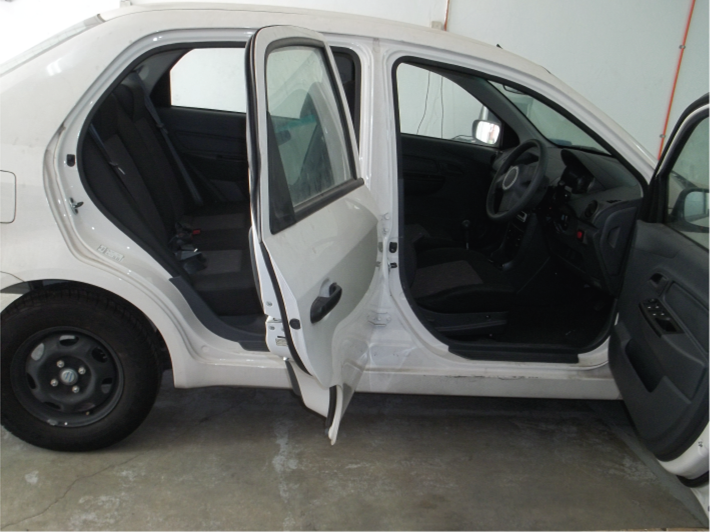
The car used for the experimental SEA.

Figure 8:

Measurement setup for experimental SEA in the car cabin.

Figure 9 shows positions of response microphone in the car cabin to measure the sound energy level. The response microphone locations were selected randomly to represent the average sound field in the subsystem, that is, at the ear and knee of passenger, above the floor, in front of dashboard, near the side windows, and near the floor.

Figure 9:

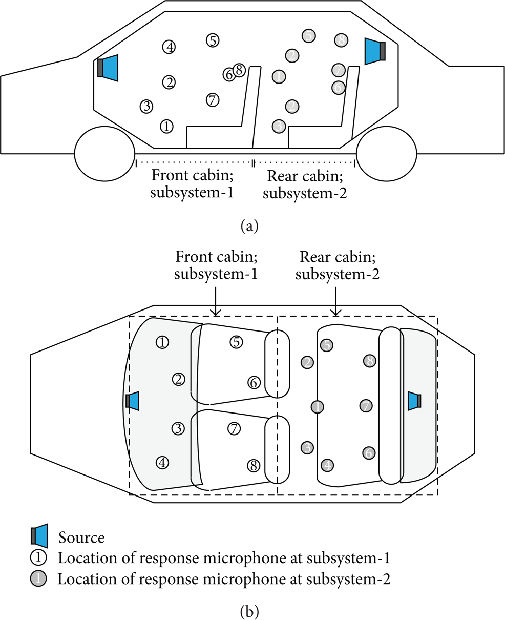
Position of reference microphones in the car cabin during measurement: (a) side view and (b) top view.

The loudspeaker was located in the front dashboard for injecting sound power in subsystem-1 and the rear dashboard for subsystem-2. The front seats were treated as the coupling between the two subsystems. For the system to have a weak coupling, there should be difference in energy level between the front and the rear cabin. Figure 10 shows the energy in one-third octave band in each subsystem when the sound source is in the front cavity (subsystem-1) and the rear cavity (subsystem-2). These are the average energy in the subsystem measured from the eight microphone positions in each subsystem as in Figure 9.

Figure 10:

Measured normalised energy in the car cabin with power injected in (a) the front cavity and (b) the rear cavity.

The difference energy level between subsystem-1 and subsystem-2 of around 5 dB can be seen due to energy loss through coupling and dissipation in each subsystem. The front and rear cabins can thus be valid to be separated into two different subsystems although note must be taken that this might not be applied for other vehicle cabins.

By applying the inverse FFT to the measured FRF at each response location, the impulse response is obtained. Figure 11 shows examples of the impulse response measured in the car cabin where the direct field component is shown by a single distinct, high peak signal. By using the windowing process (see Figure 2), this direct field component was removed as shown in Figure 12.

Figure 11:

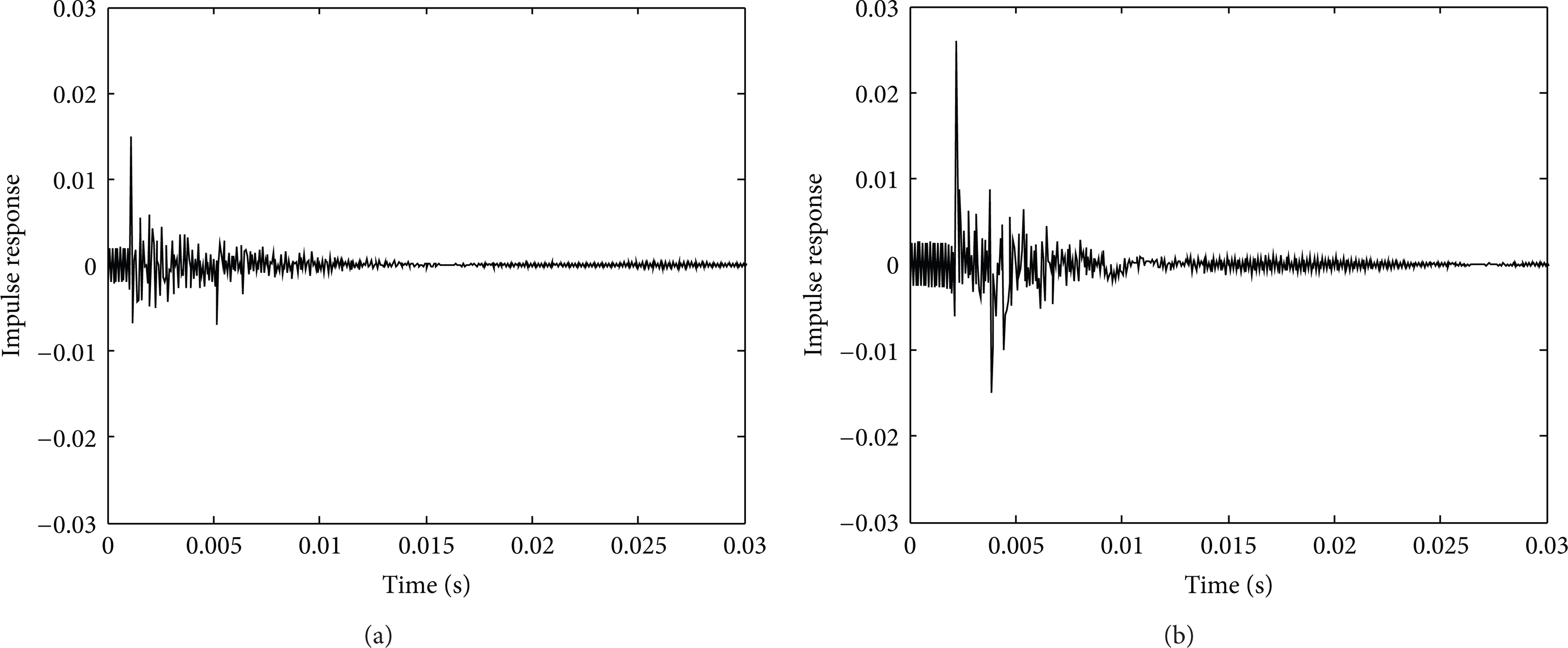
Measured impulse response in the subsystem before the direct field component removed: (a) and (b) indicate point location in the subsystem.

Figure 12:

Measured impulse response in the subsystem after removing the direct field component: (a) and (b) indicate point location in the subsystem.

The corrected FRF can be obtained by applying back the FFT to the corrected impulse response. Figure 13 presents the energy level before and after direct field correction where difference of nearly 8 dB indicates that the direct field component significantly contributes to the sound field in the car cabin.

Figure 13:

Measured normalised energy in the car cabin with power injected in (a) the front cavity and (b) the rear cavity before (—) and after (- - -) removing direct field component.

With the corrected energy in each subsystem, (10) can now be used to calculate the “corrected” DLF and CLF. This is now given by

$\left[\begin{array}{cc}{\eta }_{\mathrm{1}}+{\eta }_{\mathrm{12}}& -{\eta }_{\mathrm{21}}\\ -{\eta }_{\mathrm{12}}& {\eta }_{\mathrm{2}}+{\eta }_{\mathrm{21}}\end{array}\right]=\frac{\mathrm{1}}{\omega }\left[\begin{array}{cc}{P}_{\mathrm{1}}^{\left(\mathrm{1}\right)}\left(\mathrm{1}-\alpha \right)& \mathrm{0}\\ \mathrm{0}& P_{\mathrm{2}}^{\left(\mathrm{2}\right)}\left(\mathrm{1}-\alpha \right)\end{array}\right]{\left[\begin{array}{cc}{E}_{\text{rev},\mathrm{1}}^{\left(\mathrm{1}\right)}& E_{\text{rev},\mathrm{1}}^{\left(\mathrm{2}\right)}\\ E_{\text{rev},\mathrm{2}}^{\left(\mathrm{1}\right)}& E_{\text{rev},\mathrm{2}}^{\left(\mathrm{2}\right)}\end{array}\right]}^{-\mathrm{1}},$

(13)

where the average absorption coefficient $\overline{\alpha }$ is determined using a Sabine formulae

$\overline{\alpha }=\mathrm{0.1611}\frac{V}{S{T}_{\mathrm{60}}}$

(14)

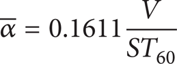
for T₆₀ is the reverberation time measured using dB-Solo analyzer, V is the volume of the corresponding subsystem, and S is surface area of the interior.

Figure 14 shows the measured sound absorption coefficient where the average value is 0.7–0.8 indicating that the car cabin has sufficiently high sound absorption. For this condition, the direct field dominates the acoustic response.

Figure 14:

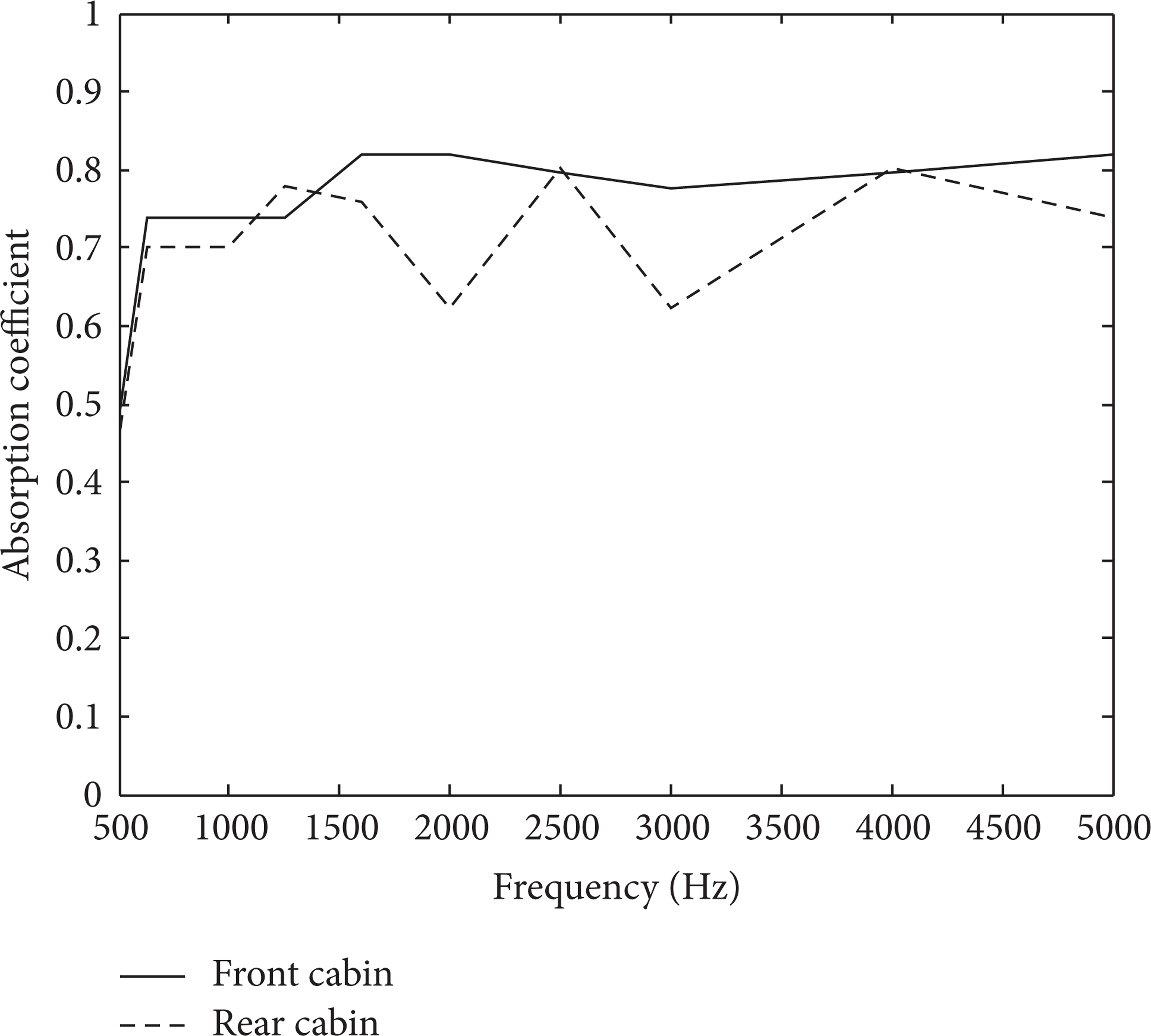
Measured sound absorption coefficient of the car cabin.

The measured reverberation time can also be used to determine the damping loss factor at subsystem-1 and subsystem-2 by using

$\eta =\frac{\mathrm{2.2}}{f{T}_{\mathrm{60}}},$

(15)

where f is the frequency.

Figure 15 presents the damping loss factor in the front cavity (subsystem-1) before and after removing direct field component in the energy by using (13). It can be seen that the measured DLF before removing the direct field component by using the conventional SEA overestimates the theory by nearly 5 dB. Good agreement with the measured DLF using measured T₆₀ as in (15) can now be seen for the measured DLF after removing the direct field component by using the corrected SEA particularly above 1 kHz. As mentioned in Section 2.1, since the volume of the car cabin is relatively small, the agreement at low frequencies is difficult to achieve due to the nature of the room mode (having very low modal density) [14] which still does not satisfy (3) although correction of the reverberant energy has been made. Based on the measured reverberation time and the volume of the cabin, the Schroeder frequency [12] is around 330–440 Hz where, above this frequency, diffuse field in the cabin is expected. All the data in this report, however, is plotted from 500 Hz to represent the results slightly shifted above this transition frequency and to take into account only the contribution of the airborne noise (discussed later in Section 4.1).

Figure 15:

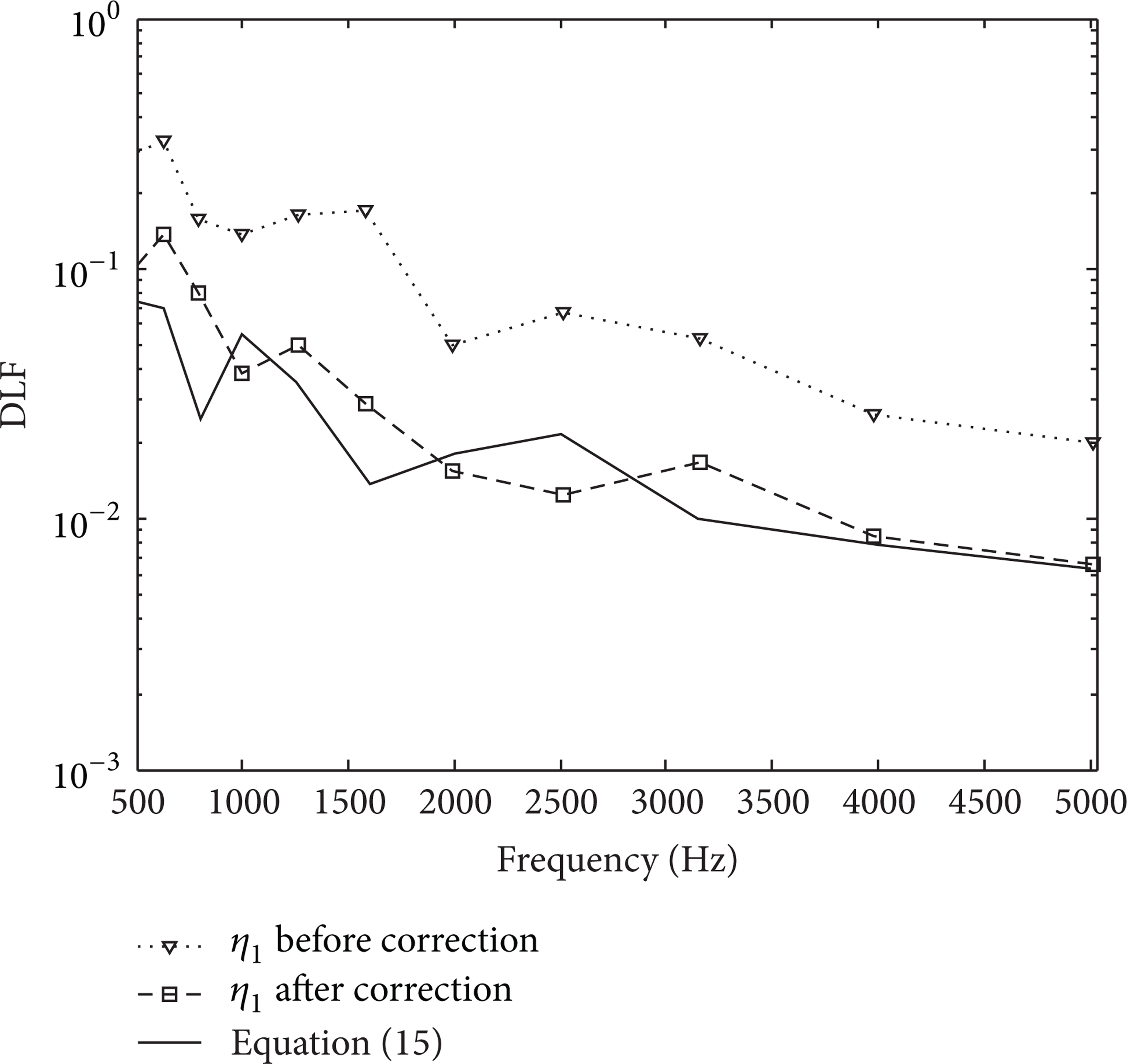
Measurement damping loss factor in the front cavity of car cabin before and after removing direct field component.

Figure 16 shows the damping loss factor in the rear cavity (subsystem-2). Again, poor agreement can be seen between the measured DLF and that from (15) before direct field correction. The corrected DLF in Figure 16 shows good agreement with the result from (15) except at 2 kHz and 2.5 kHz where this underestimates the theory by roughly 2 dB.

Figure 16:

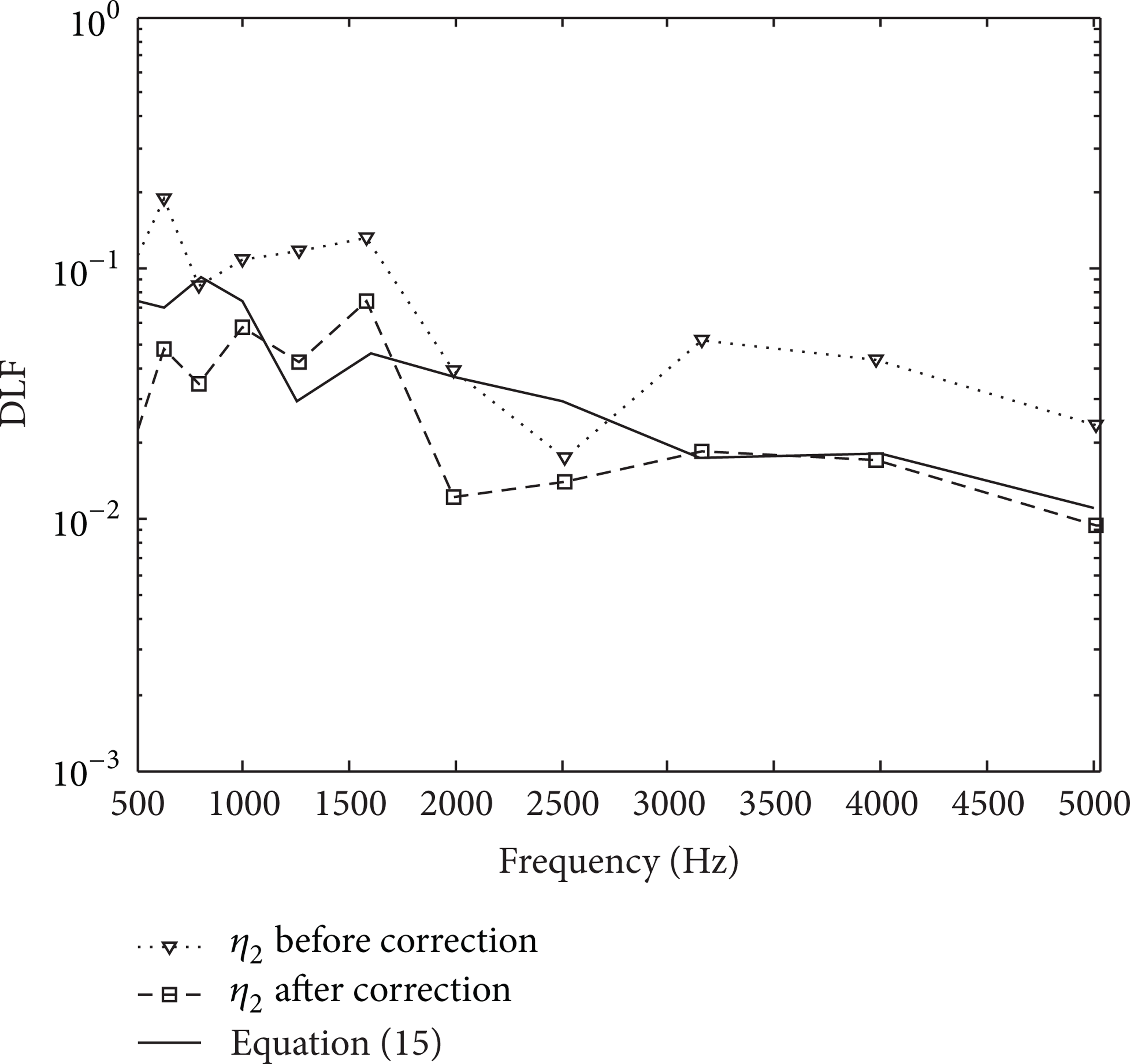
Measurement damping loss factor in the rear cavity of car cabin before and after removing direct field component.

Figures 17 and 18 present the coupling loss factor from the front cavity to rear cavity (η₁₂) and rear cavity to front cavity (η₂₁) before and after correcting the direct field component. It can also be seen here that the corrected CLF can differ by 5–6 dB between 1 and 3.5 kHz with that obtained from the conventional SEA.

Figure 17:

Measured CLFs from front cabin to rear cabin before and after removing the direct field component.

Figure 18:

Measured CLFs from rear cabin to front cabin before and after removing the direct field component.

4. Comparison with Direct Measurement of Sound Pressure Level

4.1. Measurement of Sound Power from the Engine

Measurement of the sound power level from the engine to the car cabin was conducted using the sound intensity method, following the precision method for measurement by scanning of surface [15]. The sound intensity is obtained in the frequency domain from the imaginary part of the cross-spectrum from the two closely spaced microphones in the intensity probe. The sound intensity can be calculated as [16]

$I_r=\frac{\mathrm{Im}\left(S_{\mathrm{12}}\right)}{\omega \rho \Delta r},$

(16)

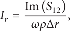
where Im ⁡ (S₁₂) is the imaginary part of the cross-spectrum from the two microphones, ρ is the density of air, ω is the angular frequency, and Δr is the distance between the surfaces of the two microphones.

The scanning was performed in front of the bulkhead area of the cabin with scanning area of roughly 0.7 m² as seen in Figure 19. Figure 20 plots the measured sound power in dB unit for different constant engine speeds. It can be seen that, above 500 Hz, the sound power which penetrates the cabin increases by 10 dB as the speed is increased. At these frequencies (usually above 400–500 Hz), the noise in a car cabin is mainly from the contribution of airborne noise [17]. The frequency range used in this report, that is, above 500 Hz, therefore represents only for the case of noise from the airborne transmission in the car.

Figure 19:

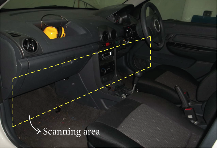
Scanning area for measurement of sound power using sound intensity.

Figure 20:

Measured sound power in car interior.

4.2. Determination of the Sound Pressure Level (SPL)

Having conducted the sound power measurement from the engine, the sound energy flowing between the subsystems, that is, the passenger cabin, can now be determined using the DLF and CLF obtained either from the conventional or corrected SEA models. The sound energy is represented here with the squared pressure defined as

$〈p^{\mathrm{2}}〉=\frac{E_i\rho c^{\mathrm{2}}}{V_i},$

(17)

where V _i is the volume of the ith subsystem and E _i is the energy calculated from the power balanced equation (see again (10)) given by

$\left[\begin{array}{cc}{E}_{\mathrm{1}}^{\left(\mathrm{1}\right)}& E_{\mathrm{1}}^{\left(\mathrm{2}\right)}\\ E_{\mathrm{2}}^{\left(\mathrm{1}\right)}& E_{\mathrm{2}}^{\left(\mathrm{2}\right)}\end{array}\right]=\frac{\mathrm{1}}{\omega }\left[\begin{array}{cc}{P}_{\mathrm{1}}^{\left(\mathrm{1}\right)}& \mathrm{0}\\ \mathrm{0}& P_{\mathrm{2}}^{\left(\mathrm{2}\right)}\end{array}\right]{\left[\begin{array}{cc}({\eta }_{\mathrm{1}}+{\eta }_{\mathrm{12}})& -{\eta }_{\mathrm{21}}\\ -{\eta }_{\mathrm{12}}& ({\eta }_{\mathrm{2}}+{\eta }_{\mathrm{21}})\end{array}\right]}^{-\mathrm{1}}.$

(18)

From (18), the energy at subsystem-1 due to the power injected in subsytem-1, E₁⁽¹⁾, can then be calculated.

By using (17), the sound pressure level is determined by

$\text{SPL}=\mathrm{10}\times \text{lo}{\text{g}}_{\mathrm{10}}\left(\frac{〈p^{\mathrm{2}}〉}{p_{\text{ref}}^{\mathrm{2}}}\right),$

(19)

where p_ref = 2 × 10⁻⁵ Pa is the reference sound pressure.

Figure 21 shows comparison between SPL from the classical SEA and the corrected SEA compared with the direct measurement of the SPL averaged over the same points in the front cavity as in Figure 9. The volume of the front cavity is around 1.05 m³ and with surface area of 6 m². Again, it can be seen that the SPL using the corrected SEA model gives better agreement with the direct measurement than that from the conventional SEA model where, for the latter, the deviation is due to the effect of the direct field components.

Figure 21:

Estimated SPL in the front cavity from classical SEA and corrected SEA compared with direct measurement: (a) 1000 rpm, (b) 2000 rpm, and (c) 3000 rpm.

5. Conclusions

A new approach in statistical energy analysis (SEA) has been used to estimate the sound pressure level in a car cabin, an acoustic subsystem with nonreverberant condition where the direct field component is dominant in the subsystem energy. The model eliminates this direct field component from the total sound energy and the conventional SEA equation is modified to account only the first reflection of the input power. The car cabin was divided into two subsystems, that is, the front and the rear cabins, by treating the front seats as the coupling components between the two subsystems. Estimation of the sound pressure level (SPL) in the car interior has been shown to give more accuracy by using the corrected SEA model, where comparison with the directly measured SPL shows good agreement.

More validations are required to test the robustness of the proposed corrected SEA model, for example, experiment in a more damped acoustic space such as in a luxury car. For a larger vehicle acoustic space such as the cabin of a bus, the transition frequency can be down to a lower midfrequency (below 400 Hz) where the structure-borne noise in this frequency range will be dominant rather than the airborne component. The choice of the substitution source to inject the acoustic power into the cabin to obtain the measured SEA parameters will be of interest. Radiation from a vibrating panel could be used to represent the structure-borne source, but the power level must be ensured to be sufficiently high to generate the acoustic modes in the cabin.

Disclosure

The authors declare that no financial relation exists either directly or indirectly between the authors and the commercial entities mentioned in the paper.

Conflict of Interests

The authors declare that there is no conflict of interests regarding the publication of this paper.