Sage Journals: Discover world-class research

Abstract

As an integrated kind of railway signal-control pattern, the four-aspect fixed autoblock system has been used in many train control systems. This paper takes the four-aspect fixed autoblock system as the research object and proposes the cellular automata model of the fixed autoblock system based on the existing theoretical researches on different train systems and traffic systems by means of the analytical study of the classical cellular automata model. The CA (cellular automata) models combine complexity of passenger railway line with the theory of cellular automata and introduce some new CA models into the existing control systems. After analyzing the relevant simulation results, we study thoroughly and obtain efficiently the needed data for the variation of the section carrying capacity, the average train delay and the train speed which have been affected by redundant time on the operation of passenger trains with different speeds.

1. Introduction

In China, there are usually many different speed trains operated in the high-speed railways. Naturally, there are many train operation organizing methods for the different organizational conditions. However, the current railway transport capacity in China still cannot satisfy the huge gap of the transportation requirements. If one train delays, it will make a domino effect for the whole system, which would result in even a worse situation: the more insufficient capacity of the railway transportation. The high speed railway transport system is so complex that it is impossible to describe it completely with the traditional methods and existing theories. The cellular automaton (CA) model is one of the most efficient ways to research the very complex systems and it can simulate the dynamic characters of the train control systems.

Many scholars have researched the train operation and organization thoroughly. Carey and Kwieciński, for example, think that, in the train planning and timetabling, the trip time on each link is assumed to depend on the type of train and characteristics of the link and conduct detailed stochastic simulation of the interaction between trains as they traverse sections of the link [1]. Abbink et al. provide a model that can be used to obtain an optimal allocation of train types and subtypes to the lines [2]. Higgins et al. present the analytically based models designed to quantify the amount of delay risk associated with each track segment, the trains, and the scheduling as a whole [3]. Fretter et al. studied the balance of efficiency and robustness in the long-distance railway timetables (especially the current long-distance railway timetable in Germany) from the perspective of synchronization, exploiting the fact that a major part of the trains run nearly periodically [4]. Hallowell and Harker researched the problem of predicting on-time performance on a partially double-tracked rail line with scheduled traffic, while Monte Carlo used simulations to validate the predictions made by the proposed model under an optimal meet/pass planning process [5]. Johanna provides an overview of the research in railway scheduling and dispatching and found that the distinction is made between tactical scheduling, operational scheduling, and rescheduling [6]. Davidsson et al. provided a survey of the existing research on the agent-based approaches to transportation and traffic management and focused on freight transportation mainly [7]. Blum and Eskandariandiscussed a new method to optimize train path for the freight railway traffic, and the methods were tested in a realistic simulation program on portions of the Burlington Northern and CSX railways [8]. Li et al. used simulation to investigate driver's responses to by-line signals and traffic signs at various approach speeds and researched the relationship between the signals and speeds [9]. Martocchia et al. found that the LEDs (light-emitting diodes) are becoming more and more common in the safety signals for the ordinary railway and described that the temperature variations depend on the changes of LED intensity and color shift [10]. Kanai et al. examined the nature of the capacity on a railway network and identified the key features of the rail timetables and the track access rights that need to be accommodated in any capacity allocation mechanism and described the three basic allocation methodologies (namely, administered/rule-based, cost-based, and market-based methodologies) and how they have been applied to the UK rail network [11].

In China, Fu et al. propose a cellular automata model to simulate the traffic flow to analyze how the length of the speed-limited section, the train time interval, and the speed-limit values affect the traffic flow. The reasonable decrease of the length of speed-limited section, the moderate increase of train time interval, and the favorable increase of the speed-limit value can improve the green light run-time of the trains [12]. Li et al. propose a lot of CA models used on the railway system. They analyzed the characteristic of traffic flow of trains under four fixed-block systems. They also simulated the train operation [13 –15]. Tang et al. propose a cellular automaton (CA) model for the movement simulations under the mixed traffic conditions. Though the aspects of these results are not for railway, the CA models of these results have strong impacts on the train's system model construction [16 –18]. Qian et al. proposed a cellular automaton traffic model for the four-aspect fixed autoblock systems and simulated the traffic phenomenon of train delay. They also investigated the effects of the main factors including train interval, proportion of freight train, dwell time of the train in the station, and the number of platforms [19 –23]. Wang et al. analyze the train systems under the moving block system by using the CA model. They proposed a new CA model to simulate the trains and achieved the needed data for the variations of section carrying capacity and the average train delay [24]. Zhou et al. put forward a cellular automaton model which is used to solve the multispeed running system of the automatic blocking section and analyzed the influence of the different speed train composing rate and the overtaking distance on transporting capacity of railway section [25]. Ge et al. put some new CA models for the intelligent transportation system, which offers much more experiences for CA model of train systems [26, 27]. He et al. put an improved CA model for the urban transportation system which takes the traffic lights and driving behavior into consideration. He provides some new CA models which can be referred to the train system research [28].

In conclusion, there are many scholars who have studied the traffic system, especially railway system by using CA model. However, less achievement at the aspect of the effects of redundant on railway has been accomplished to date.

2. The Organization of Fixed Autoblock System

The fixed autoblock system is composed of the block sections, which are marked off on intervals with a certain length on the track, and one block section can be considered as the minimum headway. Four signals can be displayed by the signaling of the four-aspect fixed autoblock system: red, yellow, yellow-green, and green. When a block section is occupied, the red signal would indicate that this section has been occupied by a train. If the block section is empty, other colored signals will be displayed by the signal lamp, as is shown in Figure 1.

Figure 1:

Principle of the fixed block control.

As a free section, a green light is displayed with the intention of reminding section, indicating that the train is allowed to enter the next section at the maximum operating velocity. A yellow-green light is displayed when entering the first braking zone; meanwhile, the velocity of the train should be reduced to the limit speed in accordance with the corresponding level when the train is going to pass through the signaling. A yellow light is displayed when entering the second braking zone; the train should start to be decelerated in this section. In the protective section, when the red signal light is displayed, the speed of the train should be reduced to 0 when approaching the signaling. This is such a process in which the train speed first reduced from $V_{1}^{\max}$ km/h to the limited speed $V_{1}^{\lim}$ and then gradually reduced to 0 and the process is accomplished successfully. With this progress, it can be ensured that a safety interval of at least two block sections existed between two trains in following operation.

3. The Cellular Automata Model of the Four-Aspect Fixed Autoblock System

3.1. Model Description

The system is simplified in accordance with the following conditions: only two different speed grades are considered in this system; the passenger trains with high-speed might take over the trains with low-speed; it allows the low-speed trains to stop at an intermediate station and wait for the high-speed trains to pass through and then start off at the right time from the intermediate station; the capacity of the intermediate station is unlimited. The effect of repairing “skylight” is ignored when the trains are running in the simulation section. The spacing between stations and the length of the block sections are equal in the simulation section. Assume that the originating station is 0 and this station does not occupy any space in the system; the other stations will occupy certain spaces because of the parking process.

3.2. Variable Description

D_station indicates the station spacing of the simulation section;

L_block indicates the length of the block section;

L_safe indicates the minimum safety distance;

r_mixed indicates the mixture ratio of the two types of trains, which is determined by the proportion of the high speed passenger trains;

$V_{j}^{\max}$ indicates the maximum velocity of the two types of trains, j = 1, 2(j = 1 indicates high speed passenger trains and j = 2 indicates low-speed passenger train);

$V_{j}^{\lim}$ indicates the limit velocity of the two types of trains, j = 1, 2 (j = 1 indicates high speed passenger trains and j = 2 indicates low-speed passenger train);

V_num(t) is the real time velocity of train num at time t;

X_num(t) is the displacement of train num at time t;

X_last(t) is the displacement of the train nearest to the originating station at time t;

l is the length of the trains;

a_j indicates the acceleration of train j; b_j indicates the deceleration of train j, j = 1, 2 (j = 1 indicates high speed passenger trains and j = 2 indicates low-speed passenger train).

3.3. The Establishment of the Model

3.3.1. The Generation of Trains

The train will be generated according to the preset train mixed ratio r_mixed. Number the train as num = num + 1; the initial velocity and the initial displacement of the train are set to be 0. For an outgoing train generated, when the front section is idle, the train will participate in the system upgrading according to the model updating rule; when the front section is occupied, the departure condition must be judged by using the following conditions.

For a high speed passenger train, it can depart only if there are 4 or more block sections between this train and the front train; otherwise, it has to keep waiting until the departure conditions are satisfied.

For a low-speed passenger train, it can depart only if there are 3 or more block sections between this train and the front train; otherwise, it has to keep waiting until the departure conditions are satisfied.

The calculating formula for the block sections between trains is as follows:

n = ⌈ \frac{(X_{last} - l)}{L_{block}} ⌉ .

(1)

3.3.2. The Updating Process of the Speed and Displacement of the Train

The speed of the train is controlled in accordance with the signals in the running process, and the display of the signals is in accordance with the occupancy/idles of the section. Therefore, the signal displayed can be obtained through the following steps:

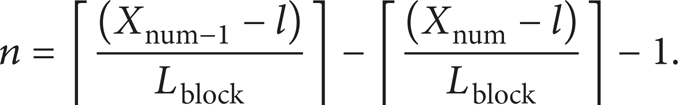
n = ⌈ \frac{(X_{num - 1} - l)}{L_{block}} ⌉ - ⌈ \frac{(X_{num} - l)}{L_{block}} ⌉ - 1 .

(2)

Here n is the number of the block sections between adjacent trains.

Calculate the updated speed of the traind

When n ≥ 4,

V_num(t) = V_num(t − 1) + a_j;

V_num(t) = min(V_num(t), V_max)

(to prevent the speed from exceeding the maximum driving speed).

When n ≤ 2,

V_num(t) = V_num(t − 1) − b_j;

$V_{num} (t) = \min (V_{num} (t), V_{j}^{\lim})$

(the speed of the train is reduced to the limit speed corresponding to the yellow-green signal).

When n ≤ 1,

V_num(t) = V_num(t − 1) − b_j;

V_num(t) = max(V_num(t), 0)

(the speed of the train is reduced to the limit speed corresponding to the yellow-green signal).

Update the displacement of the train: X_num(t) = X_num(t − 1) + V_num(t).

3.3.3. The Judgment of Overtaking

When trains of different speed grades operate in one section, there will be a situation of high-speed passenger trains following low-speed trains. To avoid this situation, the judgment conditions in this model are as follows.

When a high speed passenger train follows a low-speed train and the two trains are in the same section, we should determine whether the space between these two trains is smaller than the length of two block sections or not after a certain time interval:

T_{P} = \frac{(X_{front} - X_{following} - 2 \times L_{block})}{(V_{front} - V_{following})} .

(3)

The subscripts of “front” and “following” indicate the low-speed train in front and the high speed passenger train following, respectively;

X_front indicates the current displacement of the low-speed train in front;

X_following indicates the current displacement of the high speed passenger train following;

V_front indicates the current velocity of the low-speed train in front;

V_following indicates the current velocity of the high speed passenger train following.

The calculated time T_P is the time needed for the space between the two trains being reduced to the length of two block sections:

X_{P} = T_{P} \times V_{following} .

(4)

X_P is the expected location of the high speed passenger train after the time interval of T_P; if X_P reaches one-half of the length of the interstation section, the low-speed train must stop at the station in front to be overtaken by the high speed passenger train.

If the two trains are separated by a station into different sections, the above method is still applicable, except for the judgment of the displacement section for stopping and waiting.

3.3.4. Judgment of Departure from the Intermediate Station

After the passing through of high-speed passenger trains, the low-speed trains stopping and waiting at the intermediate station should also depart in order at appropriate time to prevent potential operation conflict.

Judgment Conditions for following Train Departure. The judgment conditions for following train departure should be determined according to the speed level.

(a) The following Train is a High Passenger Train. If the following train in the adjacent following section is a high speed passenger train, the outgoing train should be prejudged.

Assuming that both the high speed passenger train and the low-speed train are running at the maximum speed, if the distance between the two trains is equal or less than 2 L_b, and the low-speed train is within the affecting zone of the high speed passenger train, the low-speed train cannot be departed, and vice versa.

(b) The following Train is Low-Speed Train. The low-speed train can be departed if the difference between the displacement of the predeparted train and the following train is not less than 4 L_b.

Judge Conditions for Front Departure. The front departure condition of the low-speed train at the intermediate station is the same as that of the originating station.

3.3.5. Run out of the System

If the displacement of the train satisfies X_num ≥ N × L_station, then the train will be off the system.

4. Simulation and Analysis under the Condition of Different Speeds Passenger Train Traffic System

4.1. Variables

According to the above model, the parameters of each train are set as follows.

Assume the length of the block section L_block is 1000 m and the minimum safety distance L_safe is 200 m; the maximum operation velocity for high speed passenger trains $V_{1}^{\max}$ and low-speed trains $V_{2}^{\max}$ is set to be 40 m/s and 30 m/s, respectively. The limit speed for high speed passenger trains $V_{1}^{\lim}$ and low-speed passenger trains $V_{2}^{\lim}$ is set to be 28 m/s and 21 m/s, respectively. The length l of each train is set to be 200 m. The acceleration for high speed passenger trains a₁ and low-speed passenger trains a₂ is set to be 0.4 m/s² and 0.25 m/s², respectively. The deceleration and the acceleration are the same for both high and low speeds passenger trains, b₁ = a₁, b₂ = a₂.

For each parameter program, set the number of time steps for the operation of the simulation model as a total of 10800 and then take the average of all the analysis variables as the performance estimating value of the system after multiple operations.

4.2. Simulation Analysis

4.2.1. Simulation Analysis on the Actual Train Graph

As can be seen from Figure 2, because the trains running in the system are the two kinds of passenger trains with high speed, the train paths layout of the actual train graph is very dense under the condition of signal control. As there is no buffer area existing between the trains during running process, the delay of one front train will result in the successive delay of the following trains. Trains running in the system are at high speed, so the effect of low-speed trains on high-speed trains is very minor. Although the interference of delay is relatively less than the case of mixed passenger and freight line, the interference of back propagation is still being widespread.

Figure 2:

The actual intensive burst train graph under conditions of fixed autoblock.

A redundant time of 30 seconds is added to the minimum departure interval required by the four-aspect fixed autoblock system. Compared to the actual train graphs obtained previously, the delay propagation effect in Figure 3 is relatively weaker due to the speed characteristics of the trains running in the system. When two kinds of trains with speeds varying greatly mixed running in the system, the low-speed trains will greatly affect the speed of high-speed trains in the running section, and the spread range of the effects will be very wide. When the speed differences between the two kinds of trains are little, the interaction between the trains will be weak, and the propagation range will be small, too. In contrast, when trains of different speeds are running in the system under the same external operating conditions, the redundant time required will be different as well: the greater the difference between the speeds of the trains, the longer the redundant time needed and vice versa.

Figure 3:

The actual train graph under conditions of fixed autoblock considering the redundant time.

4.2.2. The Effect of the Redundant Time on Passing Capacity

The train transporting capacity Figure 4 exhibits the strong regularity: if the transporting capacity is improved with the increase of the mixed ratio and no interleaving occurs between these curves, this indicates that the interaction of the mixed trains is slight when the speed difference is minor. Passing capacities under different redundant time are distinct. When the redundant time is 0, the number of trains passing through is 42 for the mixed ratio of 0.1, and the number will reach 49 with the mixed ratio of 0.9, with 7 trains increased. The growth rate for the passing capacity under other redundant times is lower than in this case, indicating the effect of the mixed ratio is slight on passing capacity. This is completely different from the case of the mixed passenger and freight line with big speed difference, where the effect of the mixed ratio is significant.

Figure 4:

The dependence of the train passing capacity on the mixed ratio.

The passing capacity in Figure 5 is directly affected by the redundant time and can be reduced significantly. When the mixed ratio is 0.9, the number of trains passing through is 49 with the redundant time of 0, and the number is reduced to 31 with the redundant time of 120 seconds, reduced by 18 trains. It can be inferred from the comparison that the effect of redundant time on the passing capacity of bigger speed differences is greater than that of the smaller speed differences. Therefore, the redundant time should be set carefully for the mixed train line with small speed differences, so as to avoid excessive redundant time causing waste of the passing capacity.

Figure 5:

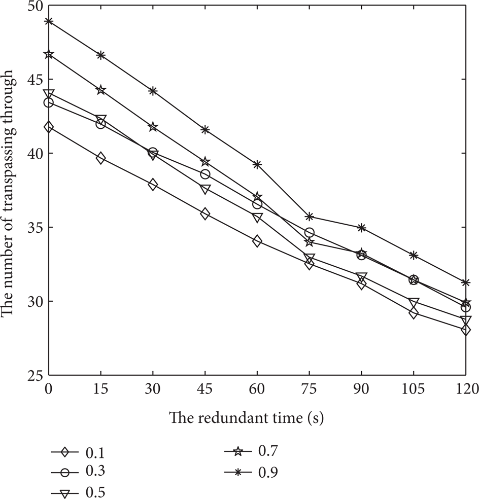
The dependence of passing capacity on the redundant time.

4.2.3. The Effect of the Redundant Time on Average Velocity

As can be seen from Figure 6, the effect of low-speed trains on high-speed trains is more significant for mixed running system with small speed differences. For mixed running system with small speed differences, the stability of the average velocity of the high-speed trains is very poor, and it will be difficult to describe the tendency of the curves with redundant time of 0 second, 15 seconds, and 30 seconds by using a certain law. When the redundant time increased to a certain degree, the average speed of the high-speed trains begins to be stabilized and will be maintained at a high level, indicating that the redundant time exerts an important influence on the stability of the system.

Figure 6:

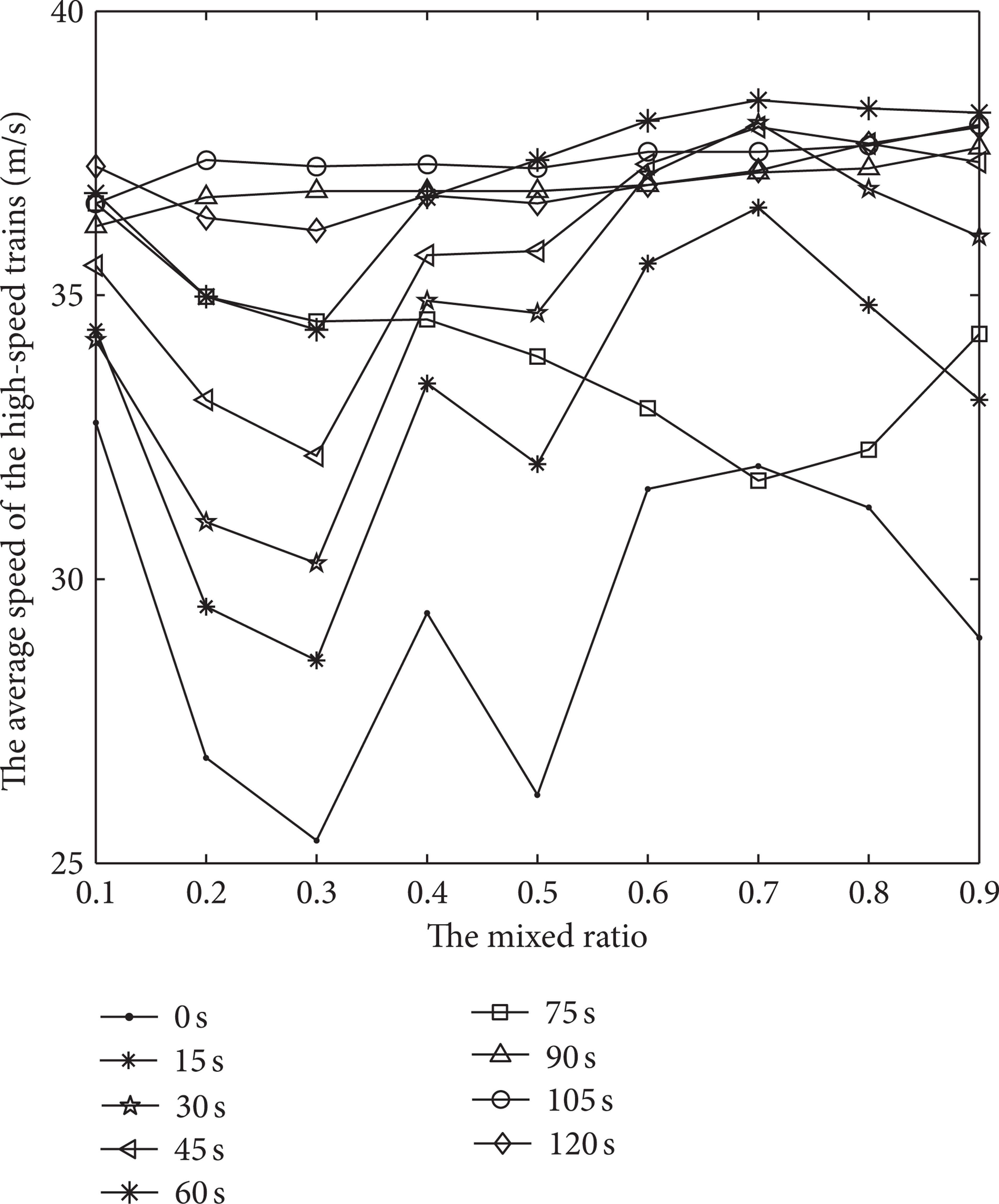
The dependence of the average speed of the high-speed trains on the mixed ratio.

As shown in Figure 7, the average speed of high-speed trains is at a high level when the redundant time is 0; when the redundant time increases from 0 to 60 seconds, the average speed is in a constant tendency of increasing; when the redundant time increases to 75 seconds, the average speed is suddenly decreased, indicating that the running of high-speed trains is restricted at this time. When the space between high-speed and low-speed trains increased to a certain extent, the low-speed trains will be able to continue to travel rather than giving way to and waiting for the high-speed trains until reaching somewhere ahead; the average velocity is reduced due to the effect of new overtaking locations. When the redundant time is between 90 and 120 seconds, the average speed of the high-speed trains in each mixed running condition reaches its peak value, and the maximum effectiveness of the redundant time is achieved, which is similar to the situation of the mixed passenger and freight line.

Figure 7:

The dependence of the average speed of the high-speed trains on the redundant time.

As shown in Figure 8, when the mixed ratio is 0.1, the average speed of the low-speed trains is between 25 m/s and 30 m/s (maximum velocity); when the majority are low-speed trains, the average speed of the low-speed trains will be at their high level and will be reduced gradually with the increase of the mixed ratio, which is totally different from the condition of mixed passenger and freight line.

Figure 8:

The dependence of the average speed of the low-speed trains on the mixed ratio.

In Figure 9, the effect of redundant time on the average speed of the low-speed trains is analyzed. For the curve of mixed ratio r = 0.1, the increase of redundant time has little effect on the overall average speed, which is relatively stable, while the redundant time is rising from 0 to 120 seconds, indicating the increase of the tracking interval has not improved the performance of the system. The tendency when r = 0.2, 0.3, 0.4, and 0.5 is similar to that of 0.1. When r = 0.6, 0.7, 0.8, and 0.9, a step occurs when the redundant time is 75 seconds. The average speed of these curves is at a lower level at the beginning and then will be improved greatly after the redundant time expanding to a certain extent and will be basically maintained at a higher level at last.

Figure 9:

The dependence of the average speed of the low-speed trains on the redundant time.

4.2.4. The Effect of the Redundant Time on the Delays

Under the condition of mixed running of trains with different speeds, the average delay of low-grade trains is reduced with the increase of the mixed ratio. The delay curves of the mixed passenger trains show slowly decaying trends with the upward bulges, and the average delay of low-speed trains is between 50 and 250 seconds; the average delay change range will be 200. By comparison, we can learn that under the condition of mixed running of passenger trains, the effect of high-speed trains on the low-speed trains is weaker than that of the low-speed trains, showing totally different trend with the mixed ratio (see Figure 10).

Figure 10:

The dependence of the average delay of the low-speed trains on the mixed ratio.

Figure 11 shows that, affected by the redundancy time, the average delay of the low-speed trains indicates the phenomenon of the grading decline, except for the proliferation when the redundancy time is 75 seconds. When the redundant time reaches 75 seconds, the overtaking relationship of the two kinds of trains will be changed as well, resulting in the further increase in the delay of the low-speed trains. In the situation of the mixed passenger and freight line, the entire system is in a steady downward trend, without signs of rebound; the deterrent effect of the redundant time on the delay spread becomes increasingly obvious with the increase of the redundant time. Under the condition of mixed passenger trains, the fluctuation of each curve becomes very slight when the redundant time reaches 90 seconds and will ultimately achieve a steady state.

Figure 11:

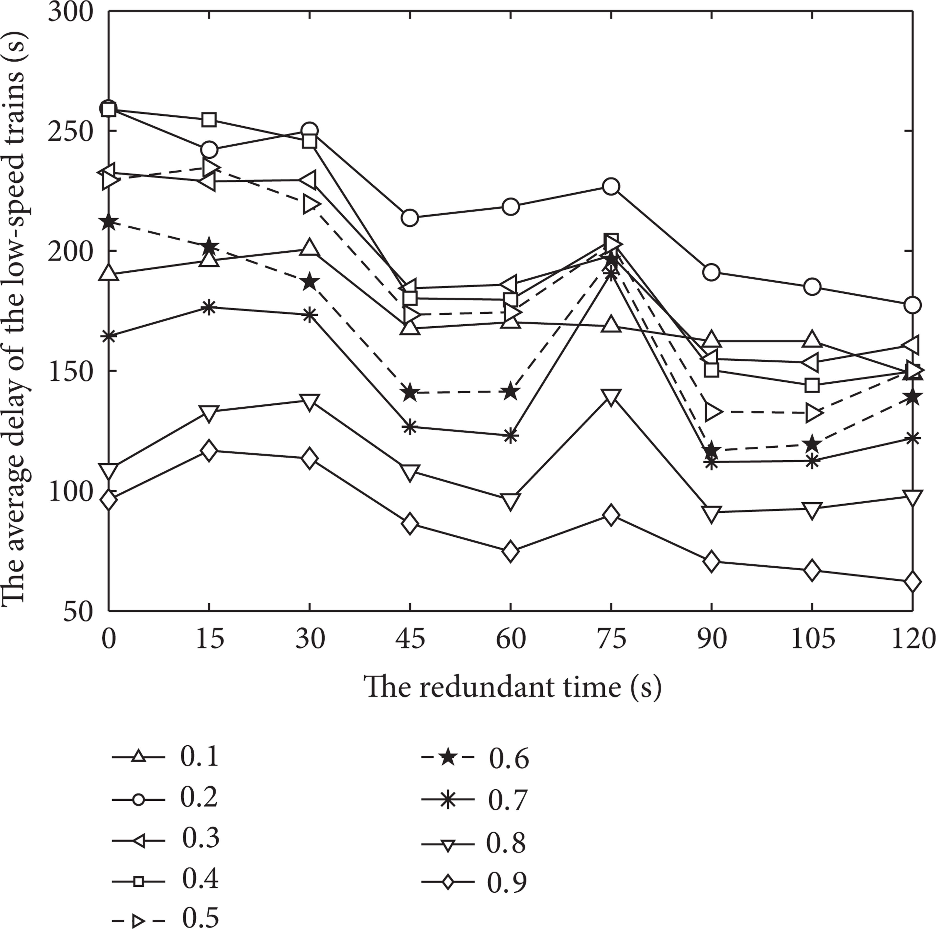
The dependence of the average delay of the low-speed trains on the redundant time.

5. Conclusions

In this paper, we establish some new cellular automaton models of mixed passenger traffic system with different speeds considering the effect of the redundant time. In this model, the redundant time is checked by signal-control system, and the departure interval is set to be a variable, so it can further improve the research on the effect of the redundant time in mixed passenger trains with different speed traffic systems. Through the CA theory, the result of simulation, which is under redundant time, portrays the rules of the train graph, the railway system's capacity and the average delay of different speed trains. The simulation process is closer to the actual operation condition of the mixed trains, which generates the transportation production, the assignment of railway carrying capacity, and the drawing of the train diagrams under the fixed block system with reference. Anyway, this work only studies the mixed railway system and the passenger trains with small speed differences. In fact, the actual situations will be more than two kinds of trains. Therefore, there are still many issues to be further studied and perfected for the actual transport system with more complex operation conditions.

Footnotes

Conflict of Interests

The authors declare that there is no conflict of interests regarding the publication of this paper.

Acknowledgments

This work is supported by the Humanities Social Sciences Programming Project of the Ministry of Education of China nos. 10YJA630126, 12YJC630200, and 12YJC630100; the State Social Science Fund Project no. 11CJY067; the Natural Science Foundation of Gansu Province, China, nos. 1107RJYA070 and 1208RJZA164.

References

Carey

and Kwieciński

, “Stochastic approximation to the effects of headways on knock-on delays of trains,” Transportation Research Part B, vol. 28, no. 4, pp. 251–267, 1994.

Abbink

Van den Berg

Kroon

, and Salomon

, “Allocation of Railway Rolling Stock for Passenger Trains,” Transportation Science, vol. 38, no. 1, pp. 33–41, 2004.

Higgins

Kozan

, and Ferreira

, “Modelling delay risks associated with train schedules,” Transportation Planning and Technology, vol. 19, no. 2, pp. 89–108, 1995.

Fretter

Krumov

Weihe

Müller-Hannemann

, and Hütt

M.-T.

, “Phase synchronization in railway timetables,” European Physical Journal B, vol. 77, no. 2, pp. 281–289, 2010.

Hallowell

S. F.

and Harker

P. T.

, “Predicting on-time line-haul performance in scheduled railroad operations,” Transportation Science, vol. 30, no. 4, pp. 364–378, 1996.

Johanna

, “Computer-based decision support for railway traffic scheduling and dispatching: a review of models and algorithms,” in Proceedings of the 5th Workshop on Algorithmic Methods and Models for Optimization of Railways, 2006.

Davidsson

Henesey

Ramstedt

Törnquist

, and Wernstedt

, “An analysis of agent-based approaches to transport logistics,” Transportation Research Part C, vol. 13, no. 4, pp. 255–271, 2005.

Blum

and Eskandarian

, “Domain-specific genetic agents for flow optimization of freight railroad traffic,” in Proceedings of the 8th International Conference on Computers in Railways, Wessex Institute of Technology, Lemnos, Greece, 2002.

Hamilton

W. I.

Morrisroe

, and Clarke

, “Driver detection and recognition of lineside signals and signs at different approach speeds,” Cognition, Technology & Work, vol. 8, no. 1, pp. 30–40, 2006.

10.

Martocchia

Papalillo

, and Spagnolo

G. S.

, “LED applications in railway signals: wavelength and intensity vs temperature variation,” Journal of Transportation Technologies, vol. 2, no. 1, pp. 78–83, 2012.

11.

Kanai

Isojima

Nishinari

, and Tokihiro

, “Ultradiscrete optimal velocity model: A cellular-automaton model for traffic flow and linear instability of high-flux traffic,” Physical Review E, vol. 79, no. 5, Article ID 056108, 2009.

12.

Y.-P.

Gao

Z.-Y.

, and Li

K.-P.

, “The characteristic analysis of the traffic flow of trains in speed-limited section for fixed-block system,” Acta Physica Sinica, vol. 56, no. 9, pp. 5165–5171, 2007.

13.

Gao

, and Ning

, “Cellular automaton model for railway traffic,” Journal of Computational Physics, vol. 209, no. 1, pp. 179–192, 2005.

14.

K. E.-P.

Gao

Z. I.-Y.

, and Ning

, “Modeling the railway traffic using cellular automata model,” International Journal of Modern Physics C, vol. 16, no. 6, pp. 921–932, 2005.

15.

Gao

Z.-Y.

, and Li

K.-P.

, “Analysis of the property of train flow in the fixed autoblock systems,” Acta Physica Sinica, vol. 56, no. 6, pp. 3158–3165, 2007.

16.

Tang

T. Q.

Huang

H. J.

, and Zhao

S. G.

, “A signal light model and its stability analysis,” International Journal of Modern Physics B, vol. 24, no. 28, pp. 5613–5623, 2010.

17.

Tang

T. Q.

Y. H.

, and Huang

H. J.

, “A macro model for traffic flow with consideration of static bottleneck,” Communications in Theoretical Physics, vol. 58, pp. 300–306, 2012.

18.

Tang

T. Q.

Wang

Y. P.

G. Z.

, and Huang

H. J.

, “A stochastic LWR model with consideration of the driver's individual property,” Communications in Theoretical Physics, vol. 58, pp. 583–589, 2012.

19.

Qian

Y.-S.

Shi

P.-J.

Zeng

, “Analysis of the influence of occupation rate of public transit vehicles on mixing traffic flow in a two-lane system,” Chinese Physics B, vol. 18, no. 9, pp. 4037–4041, 2009.

20.

Wang

Zeng

J. W.

Qian

Y. S.

, and Li

W. J.

, “Properties of train traffic flow in a moving block system,” Chinese Physics B, vol. 21, no. 7, Article ID 070502, 2012.

21.

Qian

Y.-S.

W.-J.

Zeng

J.-W.

Wang

J.-W.

, and Guang

X.-P.

, “Cellular automaton models of highway traffic flow considering lane-control and speed-control,” Communications in Theoretical Physics, vol. 56, no. 4, pp. 785–790, 2011.

22.

Qian

Y. S.

Shao

X. M.

Zeng

J. W.

, and Wang

, “An improved cellular automaton model with the consideration of a multipoint tollbooth,” Physica A, vol. 392, no. 23, pp. 5874–5878, 2013.

23.

Yuan

Qian

Y. S.

Guang

X. P.

, “The carrying capacity under four-aspect color light automatic block signaling based on cellular automata,” Modern Physics Letters B, vol. 27, no. 13, Article ID 135009, 2013.

24.

Wang

Zeng

J. W.

Qian

Y. S.

, “Properties of train traffic flow in a moving block system,” Chinese Physics B, vol. 21, no. 7, pp. 70–78, 2012.

25.

Zhou

H.-L.

Gao

Z.-Y.

, and Li

K.-P.

, “Cellular automaton model for moving-like block system and study of train's delay propagation,” Acta Physica Sinica, vol. 55, no. 4, pp. 1706–1710, 2006.

26.

H.-X.

Zhu

H.-B.

, and Dai

S.-Q.

, “Cellular automaton traffic flow model considering intelligent transportation system,” Acta Physica Sinica, vol. 54, no. 10, pp. 4621–4626, 2005.

27.

H.-X.

and Cheng

R.-J.

, “The “backward looking” effect in the lattice hydrodynamic model,” Physica A, vol. 387, no. 28, pp. 6952–6958, 2008.

28.

H.-D.

W.-Z.

, and Dong

L.-Y.

, “An improved cellular automaton model considering the effect of traffic lights and driving behaviour,” Chinese Physics B, vol. 20, no. 4, Article ID 040514, 2011.

A Study on the Effects of Redundant Time on the Operation of Different Speed-Grade Trains in Passenger Railway Line Traffic System by Using Cellular Automata Model

Abstract

1. Introduction

2. The Organization of Fixed Autoblock System

3. The Cellular Automata Model of the Four-Aspect Fixed Autoblock System

3.1. Model Description

3.2. Variable Description

3.3. The Establishment of the Model

3.3.1. The Generation of Trains

3.3.2. The Updating Process of the Speed and Displacement of the Train

3.3.3. The Judgment of Overtaking

3.3.4. Judgment of Departure from the Intermediate Station

3.3.5. Run out of the System

4. Simulation and Analysis under the Condition of Different Speeds Passenger Train Traffic System

4.1. Variables

4.2. Simulation Analysis

4.2.1. Simulation Analysis on the Actual Train Graph

4.2.2. The Effect of the Redundant Time on Passing Capacity

4.2.3. The Effect of the Redundant Time on Average Velocity

4.2.4. The Effect of the Redundant Time on the Delays

5. Conclusions

Footnotes

Conflict of Interests

Acknowledgments

References