Cluster-Based Localisation Method for Dense WSN: A Distributed Balance between Accuracy and Complexity Fixed by Cluster Size

Abstract

Localisation is a fundamental requirement for a monitoring and tracking system based on wireless sensor networks (WSN). In order to build an accurate set of measurements, sensor nodes must have information regarding their own position within a system of coordinates. When a considerable number of nodes are randomly scattered over a monitoring area, sensor nodes must be part of a self-organised system which provides a set of local position estimates. Nodes participate under very stringent conditions, for example, limited power supply and reduced computational capabilities. This work presents a GPS-free localisation method consisting of four stages that are executed only once during the network initialisation process. These stages are aimed to increase the overall system lifetime by reducing the signalling overhead commonly involved in distributed localisation procedures. The proposed localisation method turns the initial and complex node deployment to several smaller instances by dividing the network into clusters, which can be solved simultaneously based on local resources only. Simulation results show that this approach produces important savings in the involved overall complexity, which can translate into a trade-off between computational cost and localisation accuracy.

1. Introduction

Wireless sensor networks (WSN) are an emerging technology offering a wide spectrum of potential applications. However, as mentioned in [1], the adoption of this technology is limited by a set of challenging problems. From this set of problems, node localisation has been profoundly addressed and discussed by the research community because it is a fundamental requirement for monitoring and tracking (M&T) applications.

A monitoring and tracking system based on a WSN must be able to determine the source of critical events and track how these events evolve over time. In order to perform these tasks correctly, sensor nodes must have information about their own position within a system of coordinates or have accurate localisation capabilities. Position information can also be used to enhance routing decisions because nodes can send packets to their final destination based only on the position of nearby nodes, that is, knowing their neighbours’ position. These routing strategies foster local work and consequently reduce resource consumption [2–4].

For a small set of deployed nodes, individual positioning can be recorded manually. In some cases, the global positioning system (GPS) may provide a convenient starting point. GPS utilisation is nevertheless limited due to budget constraints. It is important to recall that GPS is mainly designed for outdoor scenarios without the presence of obstacles, for example, trees and mountains limiting acceptable signal reception from satellites. Alternatively, a mobile node that is aware of its own position may perform a comprehensive tour throughout the underlying network. This mobile “coordinator” may be used to inform each node about its corresponding position.

When none of the above solutions is feasible, an automatic self-configurable localisation procedure is required. Under these conditions, localisation can be understood as an inverse problem called “distance to position transformation.” If the distances among a set of nodes are known or at least estimated, a space node deployment which reproduces such collection of distances, as accurate as possible, must be found. Notice, however, that since there are three basic space isometric transformations (translation, reflection, and rotation), this statement does not ensure a single solution. In order to ensure a unique solution, a minimum set of nodes with fixed and known positions, also called beacons or anchors, is required.

Any node running a self-configurable localisation procedure needs to measure or estimate the distance between itself and its neighbours. Distance measurement techniques can be classified as range-based and range-free. Range-based techniques employ a hardware dedicated to estimate distances from a physical measurement, such as an acoustic signal's propagation time, which is then translated into Euclidean distance (ED). In contrast, range-free techniques are only based on hop count or connectivity information, which is also translated into a distance estimation. Although the latter may not achieve highly accurate results, it is a cost-effective approach that under economic constraints can be considered an appropriate alternative.

Over the last few years, an important number of approaches addressing self-configurable localisation procedures have been published. Most of them provide accurate solutions only under particular circumstances. Few of them have proven to be useful for general conditions [5–7]. However, even these general methods may show poor performance under dense node deployment. In the meantime, technology trends show that WSN have permeated different sectors of human life. The number of deployed sensors is increasing abruptly. In this context, scalability is a new borderline in current localisation methods for WSN.

The implicit agreement among scientists apparently suggests that partitioning is a promising direction to address the scalability issue [8, 9]. From this approach, the underlying network is split into clusters. Each of the resulting clusters solves a reduced version of the localisation problem. Finally, the local solutions are assembled together, like puzzle pieces, in order to build a global solution.

The method presented in this work addresses the localisation problem for a WSN comprised of a considerable number of nodes arbitrarily scattered over a given area. All nodes are assumed to be deployed at unknown but static positions with a uniform and homogeneous wireless transmission range defined by parameter R. Two nodes are within one-hop distance from each other if the distance between them is less than or equal to R. The proposed method consists of four consecutive stages that are executed only once during the network initialisation process. In Stage 1, the network is partitioned into clusters. For each of the resulting clusters there is an appointed node called leader. Cluster size, which is the number of nodes belonging to a given cluster, is controlled by a growth factor defined by each leader. In Stage 2, each leader estimates the distance between any pair of nodes belonging to the same subgraph. Distance estimations are assessed using range-free techniques. Next, the leader estimates the hop length that better translates the hop count into an estimated ED based on its local node density. In Stage 3, each leader solves a local instance of the “distance to position transformation,” which is formally known in the literature as the multidimensional scaling (MDS) problem. In Stage 4, a minimum set of anchors on each cluster is used to assemble each region into a global solution within a unique system of coordinates.

To the best knowledge of the authors, this work offers a new approach to solve the localisation problem, by introducing the following features.

• (i)

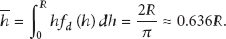
The proposed localisation method provides control over the number of nodes which are initially appointed to start the network partitioning. The number of nodes comprising each resulting cluster (cluster size) is controlled by means of a parameter, referred to as growth factor k. In turn, this parameter has an impact on the operations’ complexity in the next stages. A small cluster size produces a reduction in the exchange of control messages and calculations during Stage 2 and Stage 3, but more anchors are required to assemble the overall solution in Stage 4. If Stage 1 produces larger clusters, the opposite effect is produced.

(ii)

Once the partitioning is completed, each of the resulting clusters constructs a tree with root in its corresponding leader. Each node immediately sends a control message on its tree to the leader. These messages contain a list with the identities of the one-hop neighbouring nodes from the issuing node. Based on this information, the leader runs a centralised version of the distance vector algorithm and builds a distance matrix with the hop count between each pair of nodes lying in the cluster. This procedure also has an important benefit on the message complexity of the hop count estimation.

(iii)

To transform the hop count to an estimated ED, a naïve approach would be to multiply each hop count by factor R. Nevertheless, this decision may result in a big overall localisation error. Instead, a better correction factor of approximately $\mathrm{0.7}R$ has been estimated, approximating the average hop length. The term hop length will also be used to name this correction factor. Once the distance between each pair of nodes has been estimated, the “distance to position transformation” is solved using two different methods: eigendecomposition [10, 11] and majorisation [12]. The latter offers more leeway to achieve a compromise between position accuracy and number of iterations. In this work, higher position accuracy refers to a minimum distance between real and estimated positions.

(iv)

The proposed localisation method pays special attention to the existence of a trade-off between cluster size and the computation complexity involved in the localisation problem. Beyond raising this issue for discussion and analysis, this method also introduces a practical way to control cluster size in order to balance computation complexity. This is one of the main contributions of this work, which cannot be directly compared with previous approaches.

An evaluation of the proposed method required a computational tool that would allow an extensive set of simulation scenarios to be conducted. These scenarios consider WSN with complex settings such as a variety of sizes for the underlying graph, different node densities and transmission ranges, and the presence of obstacles. In addition, this approach is only useful for distributed implementations, forcing the sensors to find a localisation solution by themselves. Based on the previous requirements, a distributed-algorithm simulator [13] is used in order to support the implementation of the three algorithms required by the localisation method. Such method comprises network partitioning, information broadcasting, and distance-vector routing. The simulation fulfilled all previous conditions for a massive number of nodes deployed randomly. Because of the complexity of both the method and scenarios, these conditions were assessed by extensive simulation tests. However, theoretical analysis is considered not only for various sections of this work, but also for the implementation of the distributed simulation. The vast number of nodes spread over different scenarios presenting obstacles requires specific analysis that can only be performed by simulations considering multiple variables such as different network sizes and node densities, simultaneous creation of clusters, dynamic assignation of leaders for cluster, and random node distribution with uniform probability density function (PDF).

The localisation problem has already been addressed under a network scaling perspective [14–16]. For instance, in [14], the authors used the term “patches” to refer to the method of solving such a problem by dividing the network into clusters, which are then assembled to reconstruct a global solution. Nevertheless, the methods developed to solve localisation cannot be directly applied to dense node deployment, due to the excessive exchange of control messages required for these methods, which mainly reduces the sensors’ energy supply. In addition, none of the papers consulted in the literature addresses the existence of a trade-off between the cluster size and the computation complexity involved in solving the localisation problem. In contrast, beyond raising this issue for discussion and analysis, the proposed method in this work also introduces a practical way to control cluster size in order to balance out computation complexity.

The rest of this document is organised as follows. Section 2 describes the definitions and background concepts related to the proposed localisation method. Section 3 defines and explains the stages of the proposed method and presents a collection of performance assessments. Section 4 presents and analyses the results obtained from simulations. Section 5 summarises possible applications where the proposed localisation method could be used. Finally, Section 6 presents the final remarks of this work.

It is important to mention that this work is a revised and expanded version of a paper entitled “A distributed cluster-based localization method for wireless sensor networks” presented at The Sixth International Conference on Systems and Networks Communications (ICSNC 2011), Barcelona, Spain, October 23–29, 2011 [17].

2. Definitions and Background

This section formally presents the definitions and background concepts on which this work is sustained.  Abbreviation  section  summarises the variables and parameters defined or used throughout this work.

From the point of view of graph theory, a network is modelled by a graph $G=(V,E)$ , with an edge between any two nodes that can communicate directly with each other. In most cases, multihop radio networks are modelled as a unit disk graph (UDG). In a UDG $G=(V,E)$ , there is an edge $(u,v)\in E$ if, and only if, the distance between nodes u and v is less than or equal to 1, which represents a normalised wireless range.

An embedding of a graph $G=(V,E)$ in the Euclidean plane is a mapping $f:V\to {ℝ}^{\mathrm{2}}$ ; that is, each vertex $v_j\in V$ , $j=\mathrm{1,2},\dots ,n$ , is identified by a point $x_j\in {ℝ}^{\mathrm{2}}$ in the plane. A realisation of a unit disk graph $G=(V,E)$ , in the Euclidean plane, is an embedding of G such that $(u,v)\in E\leftrightarrow d(f(v),f(u))\le \mathrm{1}$ , where d is the distance between two points. Therefore, localisation consists of the realisation of a unit disk graph in the Euclidean plane.

Localisation is also considered as an optimisation problem because, given a set of measured distances between nodes that build a network, it is necessary to estimate the position of each node on a plane, up to rotations, reflections, or translations. But, at the same time, the error between real distances and the resulting distances from estimated positions should be minimised. Practitioners introduce nodes with fixed and known positions, called anchors, in order to set the system's reference coordinates.

In a sensor network, there are two types of nodes in ${ℝ}^{\mathrm{2}}$ , common sensors and anchors. A common sensor i is a node of which position has to be estimated and is denoted by $x_i\in {ℝ}^{\mathrm{2}}$ , $i=\mathrm{1,2},\dots ,n$ . In contrast, each anchor q has a well-known position $a_q\in {ℝ}^{\mathrm{2}}$ , $q=\mathrm{1,2},\dots ,m$ . Let $d_{ij}$ be the distance between a pair of common nodes i and j, and let $d_{jq}$ be the distance between a common node j and an anchor q. In some cases, there are some known and unknown values of such distances. The pairs of nodes for which their mutual distances are known are denoted as $(i,j)\in N_x$ (distance between sensor i and sensor j) and $(j,q)\in N_a$ (distance between sensor j and anchor q), respectively. In [18–20], the localisation problem in ${ℝ}^{\mathrm{2}}$ is stated as follows: given m anchor positions $a_q\in {ℝ}^{\mathrm{2}}$ , $q=\mathrm{1,2},\dots ,m$ , and some distance measurements $d_{ij},(i,j)\in N_x$ , $d_{jq},(j,q)\in N_a$ , find the positions of common sensors, such that

$$\begin{array}{cc}& {\left|x_i-x_j\right|}^{\mathrm{2}}=d_{ij}^{\mathrm{2}},\hspace{1em}\forall \left(i,j\right)\in N_x,\\ {\left|x_j-x_q\right|}^{\mathrm{2}}=d_{jq}^{\mathrm{2}},\hspace{1em}\forall \left(j,q\right)\in N_a.\end{array}$$

(1)

In many instances of the problem, noisy measurements introduce uncertainties into the previous calculations. Such uncertainties are denoted as ${ϵ}_{ij}$ and ${ϵ}_{iq}$ , respectively. Under such conditions, the problem can be reformulated as follows:

$$\begin{array}{cc}& {ϵ}_{ij}^{\mathrm{2}}=\min \left\{{\left|{\widehat{x}}_i-{\widehat{x}}_j\right|}^{\mathrm{2}}-d_{ij}^{\mathrm{2}}\right\}\\ {ϵ}_{iq}^{\mathrm{2}}=\min \left\{{\left|{\widehat{x}}_j-x_q\right|}^{\mathrm{2}}-d_{jq}^{\mathrm{2}}\right\},\end{array}$$

(2)

where, ${\widehat{x}}_i$ and ${\widehat{x}}_j$ are the estimated positions of sensors i and j, respectively.

Notice that anchors provide a fixed and absolute reference to the system. Otherwise, when there are not anchors at all, the solution shows only relative positions. In other words, the “drawing” of the solution of the original network can be rotated, reflected, or translated. For instance, in [21], the authors propose the utilisation of two anchors only in order to fix the node positions lying on a regular square. This is probably the main drawback, because it cannot be applied for the solution of arbitrary deployments.

Different techniques have been proposed to measure the distances that make up the input set of the localisation problem. These techniques can be classified into two main categories: range-based and connectivity-based techniques (also called range-free techniques). The former depend on a physical signal exchanged between two points the value of which is a function of the length, or relative position, of the line of sight from transmitter to receiver. For example, angle of arrival (AoA), time of arrival (ToA), and received signal strength (RSS).

The downside of range-based techniques is that they require additional hardware that may impact individual node price. Besides, they can be highly sensitive to environmental conditions. In contrast, connectivity-based techniques depend on the number of hops separating any pair of nodes. In this case, it is assumed that two nodes sharing an edge are separated, at the most, by one distance unit which is defined by the wireless transmission range. For both categories, indirect measurements may be propagated to other nodes in the network using a distributed procedure, such as the distance-vector algorithm (DV), where each node successively sends all the distances and the paths to reach the destinations it already knows. It is very important to consider the fact that DV has an exchanged message complexity $O(|V{|}^{\mathrm{3}})$ , where $\left|V\right|$ is the number of nodes involved.

Research on localisation techniques has produced methods that offer excellent performance when the deployed sensors make up a dense and globally uniform network. Among the most relevant pieces of research, in [14] the authors demonstrated the use of a data analysis technique called MDS in estimating unknown node positions. First, when using basic connectivity or distance information, a rough estimate of relative node distances is acquired. Then, classical MDS [10, 11] (which basically involves using eigenvector decomposition) is used to obtain relative node position maps. Finally, an absolute map is obtained by using known node positions. This technique works well with few anchors and reasonably high connectivity. For instance, for a connectivity level of 12, that is, the mean number of neighbours each sensor has, and 2% of anchors, the error is about half of the wireless range ( $R/\mathrm{2}$ ).

It is important to mention the theoretical procedures that are commonly used to solve the MDS problem. Such procedures were also implemented in the simulator in order to provide this solution. Supposing a matrix X, where each of its rows codes the position of a point on an Euclidean space, it is possible to compute the square of the distances between any pair of points in this collection, that is, $\mathbf{D}(\mathbf{X}{)}^{\mathrm{2}}$ , according to the following expression found in [10, 11]:

$$\begin{array}{cc}& \mathbf{D}{\left(\mathbf{X}\right)}^{\mathrm{2}}=\mathbf{c}{\mathbf{1}}^T+\mathbf{1}{\mathbf{c}}^T-\mathrm{2}\mathbf{X}{\mathbf{X}}^T=\mathbf{c}{\mathbf{1}}^T+\mathbf{1}{\mathbf{c}}^T-\mathrm{2}\mathbf{B},\end{array}$$

(3)

where c is a vector made up with the elements from the diagonal of $\mathbf{X}{\mathbf{X}}^T$ . By left and right multiplication of matrix $\mathbf{D}{(\mathbf{X})}^2$ by a centering matrix $(\mathbf{H})$ and by factor $-1/2$ in order to obtain:

$$\begin{array}{l}-\frac{\mathrm{1}}{\mathrm{2}}\mathbf{H}\mathbf{D}{\left(\mathbf{X}\right)}^{\mathrm{2}}\mathbf{H}=-\frac{\mathrm{1}}{\mathrm{2}}\mathbf{H}\left(\mathbf{c}{\mathbf{1}}^T+\mathbf{1}{\mathbf{c}}^T-\mathrm{2}\mathbf{X}{\mathbf{X}}^T\right)\mathbf{H}\\ =-\frac{\mathrm{1}}{\mathrm{2}}\mathbf{H}\mathbf{c}{\mathbf{1}}^T\mathbf{H}-\frac{\mathrm{1}}{\mathrm{2}}\mathbf{H}\mathbf{1}{\mathbf{c}}^T\mathbf{H}+\frac{\mathrm{1}}{\mathrm{2}}\mathbf{H}\left(\mathrm{2}\mathbf{B}\right)\mathbf{H}\\ =-\frac{\mathrm{1}}{\mathrm{2}}\mathbf{H}\mathbf{c}{\mathbf{0}}^T-\frac{\mathrm{1}}{\mathrm{2}}\mathbf{H}\mathbf{0}{\mathbf{c}}^T+\mathbf{H}\mathbf{B}\mathbf{H}=\mathbf{B}.\end{array}$$

(4)

The first two parts of (4) are cancelled out since centering a vector made up with 1s produces a vector made up with 0s only ( ${\mathbf{1}}^T\mathbf{H}=\mathbf{0}$ ). In turn, since it is assumed that the columns in X have a mean equal to 0, the centering matrices around B can be dismissed. Now, if matrix B can be factorised according to an eigendecomposition, it will turn out that $\mathbf{B}=\mathbf{Q}\mathrm{\Lambda }{\mathbf{Q}}^T=(\mathbf{Q}{\mathrm{\Lambda }}^{\mathrm{1}/\mathrm{2}})(\mathbf{Q}{\mathrm{\Lambda }}^{\mathrm{1}/\mathrm{2}}{)}^T=\mathbf{X}{\mathbf{X}}^T$ . There is a tool that carries out this decomposition: the so-called power method, which is an iterative algorithm of complexity $O(n^{\mathrm{3}})$ , where n is the number of unknown positions. In this work, an optimisation approach has also been implemented in the simulator. This approach, called the majorisation method, is also an iterative algorithm of complexity $O(n^{\mathrm{2}})$ , but it is not based on eigendecomposition.

Other related works can be found in [22, 23], where the authors present a series of distributed and iterative methods, based on neural networks, to solve the fundamental optimisation problem that lies on the core of localisation.

3. Methodology and Stage Description

The method introduced in this work is comprised of four consecutive stages: (A) partitioning; (B) hop count and distance estimation; (C) distance to position transformation; and (D) anchors deployment. It is important to point out that these stages are executed only once during the network initialisation process. The stages are described in more detail in the following subsections.

3.1. Partitioning

The partitioning methods developed by other research teams to address scalability, so far, start selecting a set of nodes; each of these appointed nodes builds its own cluster. Each cluster grows inviting its neighbour nodes to join the subgraph under construction. Nevertheless, to the best knowledge of the authors, these procedures do not control neither the cluster growth rate nor the initial number of appointed nodes. In [24], for instance, each node in the graph is regarded as a cluster, provided that it is not assimilated by a larger one. These conditions may lead to a waste of the number of messages exchanged. In addition, such simultaneous cluster construction may produce an unnecessary condition where neighbouring clusters compete for nodes that have not yet been assigned, having an impact on the number of messages exchanged. Network-partitioning message complexity may therefore turn out to be excessive.

In this work, a network-partitioning algorithm based on the γ synchronizer of Awerbuch [25] is introduced. A synchronizer is a set of techniques that enables an asynchronous system to emulate a synchronous behaviour. To support this emulation, each node should be able to proceed with the next step of the given algorithm, only when it is granted that all the participants have accomplished the preceding step [26]. A node under these conditions is said to be “safe.”

Awerbuch introduced three types of synchronizers: the α type, where each node exchanges messages with all its neighbours to let them know that it is safe. The β type uses a preconstructed spanning tree. Here, a node sends a control message to the root node when the current step has finished. Once the root node has collected these messages from each node, it broadcasts a new message back to the nodes on the tree, in order to notify the overall safety.

Finally, in the γ synchronizer the underlying graph is partitioned into a forest. Each of the resulting clusters runs a local version of the β synchronizer. However, when nodes of a given cluster have finished the current step, the root node exchanges messages with its neighbouring trees to let them know of its local condition. When a root node recognises this condition on each of its neighbour subgraphs, it broadcasts back a new message to its tree nodes in order to notify the overall safety. The γ synchronizer requires an initialisation procedure to split the underlying graph into a set of disjointed trees. The construction of a tree starts when a given node is appointed as a leader or root node. The new leader begins aggregating layers (subsets of nodes) to the tree under construction. A new layer joining the tree is expected to contain, at least, as many nodes as k times the total number of nodes already included in the tree. When this condition is not met, the tree construction stops. Then, a new leader is found and the procedure starts again. Here, there is a special link, called “preferred link,” between the former tree and the new one about to be settled. This link fixes a relationship between the “ancestor” tree and its “successor.” When a tree stops growing and a new node cannot be appointed, the leader in charge turns the control back to its ancestor tree. In due time, the receiving leader looks for a node to start a new successor tree; otherwise it also turns the control back to its own ancestor tree. According to this rule, the initial leader is able to recognise the moment when the partition is completed. Then, the graph has been exhaustively explored and each node has been incorporated to a given tree.

The partitioning technique introduced in this work is based on the γ synchronizer by using a modified version of cluster growth parameter k. While [25] does not consider the values of $k<\mathrm{1}$ , the proposed implementation supports any value of $k>\mathrm{0}$ . Nevertheless, when the partition process works under these “suboptimal” growth rates, each cluster grows at a very slow pace and average cluster size increases. The selected value of k may therefore result in a critical decision for the proposed localisation method.

Besides the partition procedure proposed in [25], here named “serial partitioning,” a new approach, named “concurrent partitioning,” is introduced into this work. In this approach, once a cluster stops growing, its border nodes select and instruct to some neighbouring nodes that are not cluster members, to start building new clusters. As a result, preferred links between such clusters are implicitly defined. In contrast to serial partitioning, in the concurrent approach, a given cluster does not turn the control back to its ancestor when there is no further place to explore. This feature does not preclude the further initiation of the next stage of the localisation method. Figure 1 shows the behaviour of the proposed serial partitioning approach for three values of k: 0.7, 1, and 2.

Figure 1

Building clusters with different values of k.

The serial partitioning approach shows similarities with the work presented in [27, 28]. In contrast, the proposed method does not have as many cluster construction rules. Potential conflicts on node assignation are solved with a very simple rule: a free node, that is, a node not yet assigned to a cluster, decides to be part of the first cluster that accepts it. Otherwise it will eventually turn into a new cluster leader on its own.

A first assessment was developed assuming that the system runs the localisation procedure without any previous partitioning. It is then run by choosing a partitioning with different orders, that is, the number of nodes on the resulting clusters. Figure 2 shows the overall message complexity associated to each test, that is, the total number of messages that need to be exchanged throughout all the four stages of the proposed localisation method. Results show that network partitioning saves expenses by several orders of magnitude.

Figure 2

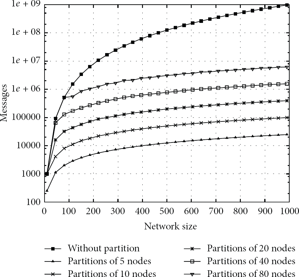
Network partitioning benefits. Total number of control messages throughout the four stages of the localisation method. The number of messages is represented as a function of network and cluster sizes.

In a second evaluation, a comparison is performed between the serial and the concurrent network partitioning approaches, for a value of $k=\mathrm{1}$ . Both have been tested over 50,000 different networks with 600 nodes each, which were generated randomly. The results provide a 95% confidence. Table 1 summarises the results of one of these experiments.

Table 1

Network partitioning benefits by means of serial and concurrent approaches.

Variables	Serial	Concurrent
Finalisation timea	809.25	213.01
Messages transmittedb	28146.73	25445.32
Transmitted messages per nodec	49.77	45.81
Leader's transmitted messagesb	1920.82	2091.70
Leader's transmitted messagesc	111.79	83.07
Number of resulting clusters	4.37	11.98
Cluster size	19.336	11.11

${}^{\text{a}}$ Assuming that a control message is transmitted using a time unit, ^baverage total number of control messages, and ^caverage individual number of control messages.

For the same set of experiments, defined in the second evaluation but now varying the value of the growth factor k, the number of resulting clusters must not exceed 14. Otherwise, the serial partitioning overperforms the concurrent partitioning in message exchange, as observed in Figure 3. This is due to the fact that, as long as the number of clusters is below this limit, less messages are required to complete the network partitioning stage. It is worth pointing out that the number of exchanged messages plotted in Figure 3 is related to this stage only. The existence of this limit can be explained as follows. Suppose that both partitioning strategies are tested in the same WSN region. If cluster size is set to a small value, the number of clusters in this region will be high. During concurrent network partitioning, where clusters are created simultaneously, there is an excessive signalling overhead due to the exchange of messages compared to serial partitioning. Under these conditions, each node in the network receives more “invitation-messages” from its neighbours but only one of them is accepted. This is translated into a waste of available resources, for example, bandwidth or battery supply. Although this condition may vary depending on network settings, similar trends may be expected like those shown in Figure 3.

Figure 3

Comparison of concurrent and serial approaches.

3.2. Hop Count and Distance Estimation

In the second stage of the method, a local instance of DV, or Bellman-Ford algorithm [29], is executed on each of the resulting clusters to calculate the shortest path between every pair of nodes lying on the same cluster. The length of each path is the first step to estimate the distance between each pair of nodes, which is required in the following stage. The routing algorithm requires the whole set of links that are part of the induced subgraph.

The DV-hop algorithm of [30] is one of the first algorithms used to estimate the distances between pairs of nodes that can be traced back in the literature. The DV-hop algorithm proposes the utilisation of hop counts between anchors to estimate such distances. In [31, 32], the authors propose considering local node density to estimate these distances. In [15], the authors include a very thorough treatment that divides a node's one-hop neighbourhood into three disjointed subsets according to their hop-count values. The integer hop-count is then transformed into a real number depending on the subset where that node lies.

In the original DV algorithm, each node exchanges control messages with all its neighbours in order to calculate the shortest path between any pair of nodes. This approach produces a message complexity $O(|V{|}^{\mathrm{3}})$ , where $\left|V\right|$ is the order of the underlying graph, that is, the total number of nodes that make part of the graph. However, in wireless sensor networks, control message transmission is an event that has a major impact on node energy supply. For this reason, an alternative approach has been developed: each node sends its neighbours list to the leader. The leader collects this information to build a model of the underlying subgraph and then runs a centralised version of the routing algorithm. This method has a complexity $O(|V|)$ on the number of exchanged messages.

In [33], the authors propose a new procedure to estimate the scaling factor of the average hop length. Their method minimizes the square mean error of the distances from each point to the set of deployed anchors. These results outperform the MDS-MAP and DV hop. Nevertheless, we consider that the amount of exchanged messages involved in this solution strongly limits its scalability.

In order to transform a hop count to an ED, a correction factor has been proposed in this work. By means of simulation, it has been found that this correction factor is about $\mathrm{0.7}R$ , which is approximately the average or mean hop length. Depending on the density of the underlying graph, there is a value that optimises the output of the following stages. These results are shown in Figure 4. In this figure, the reconstruction error is plotted for ten different hop lengths, that is, from $\mathrm{0.1}R$ to R, and for four network average densities, that is, $\mathrm{7.64}$ , $\mathrm{10.78}$ , $\mathrm{13.69}$ , and $\mathrm{15.71}$ nodes/R. The horizontal axis in Figure 4 represents normalised average hop length, whereas the vertical axis represents normalised distance estimation error. Values are normalised by dividing both distances by the wireless transmission range (R). The simulation results show that there is a hop length that minimises the MDS reconstruction error for each of these densities. It can be deduced from Figure 4 that the average hop length that minimises the distance error is between $\mathrm{0.6}R$ and $\mathrm{0.7}R$ . It can also be observed in the same figure that the distance estimation error decreases when node density increases. The analysis presented throughout the rest of this section is intended to explain such behaviour.

Figure 4

Reconstruction error varying hop length in normalised units.

In order to determine the average hop length, a wireless sensor network comprised of n sensor nodes is considered. In this network, nodes are randomly scattered over a region covering an area of $A\hspace{0.17em}\hspace{0.17em}{(\text{m}}^{\mathrm{2}})$ . In order to guarantee a high degree of connectivity among all network nodes, each sensor node must be connected, at least, with another one. This condition is fulfilled only if the distance between each pair of nearby nodes is less than or equal to the wireless transmission range. In this work, a constant transmission range, defined by R, is considered, thus leading to circular coverage zones. If a node requires establishing a communication link with another node, but the distance between this pair of nodes does not satisfy previous restriction, the presence of at least one intermediate node will be needed as a relay to retransmit the information. In order to operate as relay nodes, intermediate nodes must be found within a limited region resulting from the intersection of coverage zones defined by the wireless transmission ranges of its adjacent nodes.

Figure 5 depicts a source node (S) communicating with a destination node (D) through an intermediate node (I). Note that, in this case, the intermediate node must be located within the overlapping region of the coverage zones of nodes S and D.

Figure 5

Wireless communication involving a source node (S) an intermediate node I and a destination node D.

In [34], the authors found a closed-form expression to determine the relative distance between any pair of nodes. In [34], they also provide the PDF and CDF functions for such distance. In a one-hop communication, the relative distance d between two nodes is restricted in the interval $\mathrm{0}\le d\le R$ . For this case, the corresponding PDF would be

$$\begin{array}{cc}& f_d\left(h\right)=\{\begin{array}{cc}\frac{\mathrm{2}}{\pi }\frac{\mathrm{1}}{\sqrt{\left(R^{\mathrm{2}}-h^{\mathrm{2}}\right)}};\hfill & \mathrm{0}\le h\le R\hfill \\ 0;\hfill & \text{otherwise.}\hfill \end{array}\end{array}$$

(5)

In (5), the term h represents the one-hop distance. By computing the mean value $\overline{h}$ , it is obtained as

$$\begin{array}{cc}& \overline{h}={{\displaystyle \int }}_{\mathrm{0}}^R‍h{f}_d\left(h\right)dh=\frac{\mathrm{2}R}{\pi }\approx \mathrm{0.636}R.\end{array}$$

(6)

It is worth pointing out that the mean hop length may change according to the node density found in the network.

3.3. Distance to Position Transformation

When a leader has estimated the distances between any pair of nodes belonging to its cluster, it starts the third stage of the procedure, which solves a local instance of the MDS problem. As stated in Section 2, solving the MDS for a cluster of size n implies the transformation of a matrix $\mathbf{D}(\mathbf{X}{)}^{\mathrm{2}}$ of $n\times n$ entries, which contains the quadratic distances between each pair of nodes lying in the same cluster, into a vector X of $n\times \mathrm{2}$ entries, which encodes the node positions reproducing such distances, with the exception of possible isometries. This work evaluated three alternatives: (a) the classical eigendecomposition [10, 11]; (b) a second iterative procedure called the majorisation method, that is, scaling by majorising a complicated function (SMACOF) [12]; and (c) the combination of both. In this last procedure, a preliminary solution was built using method (a) which is further supplied as a new input to method (b). As expected, this combined approach offers the best results (see Figures 6(a) and 6(b)). Nevertheless, the second alternative offers nearly the same quality at a lower price. It is important to recall that eigendecomposition has a complexity order equal to $O(n^{\mathrm{3}})$ , where n is the number of unknown positions. In contrast, majorisation shows lower computational complexity, that is, $O(n^{\mathrm{2}})$ , and also offers a trade-off between position accuracy and number of iterations, which results in a relevant advantage for WSN, especially for nodes with limited computational capabilities.

Figure 6

Localisation error for two network densities.

Figures 6(a) and 6(b) illustrate the node localisation error for the three alternatives evaluated in this work. This evaluation involves four network node densities but only two of them are shown in Figures 6(a) and 6(b), that is, $\mathrm{10.78}$ and $\mathrm{15.71}$ nodes/R. In addition, twelve cluster sizes are considered, that is, from $\mathrm{20}$ to $\mathrm{130}$ nodes/cluster. For example, for a node density of $\mathrm{10.78}$ nodes/R and $\mathrm{100}$ nodes/cluster and using the classical eigendecomposition, the localisation error reaches $\mathrm{0.8}R$ , whereas the SMACOF method achieves a localisation error of $\mathrm{0.72}R$ and, by using the combination of both methods, the localisation error is slightly improved to $\mathrm{0.7}R$ . By observing these figures, it can also be deduced that the localisation error reduces as the network node density increases.

3.4. Anchor Deployment

When each leader has solved the local instance of the MDS, the cluster's geometric centre is considered at the position $(\mathrm{0,0})$ , or $(\mathrm{0,0},\mathrm{0})$ , whether node deployment is in 2D or 3D, respectively. This means that all clusters logically overlap. In the procedure's last stage, a minimal set of anchors is set in each cluster in order to perform an isometric transformation that fixes the final coordinates of each region. A global coherent picture of the system is thus built.

Figures 7(a) and 7(b) show localisation results without and with partitioning, respectively. The average localisation error without using partitioning exceeds $\mathrm{2.11}R$ , whereas the use of network partitioning improves the average localisation error to $\mathrm{0.645}R$ . It is worth mentioning that the proposed localisation method achieves similar results to Shang's method while only comparing the localisation error. Nevertheless, from Shang's point of view in [14], at first, each node is considered as a cluster on its own and it therefore induces an excessive exchange of control messages. In contrast, in the proposed method, message complexity is bounded by the growth factor (k) during the first stage.

Figure 7

A network reconstruction. (a) Reconstruction without partitioning. (b) Reconstruction with partitioning. In these figures, distances are measured considering a normalised wireless range ( $R=\mathrm{1}$ ).

It is important to point out that the decisions taken in Stage 1, concerning parameter k, have an impact on the further stages. There are two cases to be considered: (a) when the value of $k\ge \mathrm{1}$ and (b) when the value of $k<\mathrm{1}$ . The first case produces a large number of small-sized clusters. The second case generates a small number of large-sized clusters. A large number of clusters increase the number of anchors required during Stage 4 but reduce the computational complexity of Stages 2 and 3. The opposite effect occurs when the number of clusters is small. Finally, simulations show that small-sized clusters produce more accurate reconstruction. This is recommended for irregular areas in particular.

4. Results Analysis

This work proposes a localisation procedure consisting of four consecutive stages. In the first stage, the underlying graph is partitioned into clusters. In the second stage, each appointed starting node, that is, the cluster leader, calculates the distance in hops between every pair of nodes belonging to its cluster. Next, it translates each hop count into an estimated ED by using a correction factor, named average hop length in this work. In the third stage, each leader solves a local instance of the multidimensional scaling problem. Finally, in the fourth stage, a set of anchors is allocated to each cluster, in order to assemble each region into a coherent solution within a unique reference system. It is important to recall that, as mentioned above, these stages are executed only once during the network initialisation process.

The partitioning technique is based on a cluster growth parameter k. From the simulation results, it can be concluded that a value of $k\ge \mathrm{1}$ offers better solutions in terms of (i) time to solve stage one, (ii) a dramatic reduction of the amount of resources involved in the overall procedure, (iii) sharing the reduced overall expenses among a larger number of participants, and (iv) producing more accurate solutions.

In the downside, it is considered that the last stage limits the applicability of the method, but it has also been identified that in order to overcome this limitation it is necessary to review the connection step between neighbour clusters, during the partitioning procedure. It is known that the rigidity of a graph is a desired property that facilitates its realisation in a Euclidean space. Therefore, the more connections there are between neighbour clusters, the more rigid the resulting combined graph is [35]. If the number of links between clusters is maximised, then it is possible to use a minimal number of anchors to fix a global coordinated system.

The partitioning method works for any network, regardless of its topology and size. In fact, this partitioning stage can cope with irregularities and obstacles and is a necessary step to scale up any localisation algorithm. This is a well-known approach called “divide and conquer.” The initial and complex node deployment turns to several local instances of the original localisation problem, where it is assumed that these local instances can be solved simultaneously. In addition, although this approach enforces organisation based on local resources, it is also possible to achieve coordination in a global context.

Figure 8(a) depicts three wireless sensor networks with 200 nodes each scattered over different layouts (I-shape, O-shape, and C-shape topologies). These scenarios are intended to evaluate the localisation method under conditions that consider the presence of obstacles. Figure 8(b) shows the localisation error, which is represented by line segments traced from real to estimated positions. As indicated in Figure 8(b), the average localisation error for these experiments fluctuated between $\mathrm{0.6}R$ and $\mathrm{0.75}R$ , approximately. Depending on the scenario topology, the number of clusters must be adjusted by means of parameter k in order to reduce the localisation error.

Figure 8

(a) Three wireless sensor networks with 200 nodes and different layouts (I-shape, O-shape, and C-shape topologies). (b) Localisation errors for these scenarios. In these figures, distances are measured considering a normalised wireless range ( $R=\mathrm{1}$ ).

Node coordination is a key capability the complexity of which depends on network partitioning. If each network node were a cluster in itself, it would require exchanging messages with its immediate neighbours in order to achieve a coordinated action as proposed in the α synchronizer. Although it is a very fast strategy for node coordination, it can be very expensive in terms of the overall number of control messages sent on each link of the underlying graph. In contrast, β synchronizer can be used where a single spanning tree could be previously built on the graph. And as a result, a minimal number of control messages would be necessary to coordinate the whole system, where the time to coordinate the system would be the one needed to travel the longest path of the tree.

The γ synchronizer and the concurrent version proposed in this work find a trade-off between the number of control messages and time complexity in a coordination procedure, including the localisation process.

5. Possible Applications

The localisation method proposed in this work is suitable for critical mission applications designed for monitoring and tracking environmental conditions, for example, fire, pollution and flooding, or volcanic eruption detection. For example, the authors in [36] propose a wireless sensor network for real-time forest fire detection, which is an important issue that requires attention from different organisations and communities [37–39].

Up to now, satellite imagery has been a preferred tool to deal with monitoring and tracking environmental conditions. However, WSN emerged as a promising solution to detect environmental risks, by providing significant parameters that can hardly be obtained through using satellite monitoring. Therefore, a joint network with terrestrial sensor networks and satellites can offer an integral and effective solution.

In [7], the authors considered WSN as an excellent choice to deal with early forest fire detection but they also warned that a fire detection application using WSN requires the identification of sensors’ position as a mandatory condition. When choosing a localisation algorithm, the following performance properties should be considered:

• (i)

message exchange,

(ii)

computational complexity,

(iii)

position accuracy,

(iv)

self-configurable, scalable, and distributed capabilities.

The proposed localisation method developed in this work considers all the above-mentioned properties.

Commonly, a monitoring and tracking application may involve a large area to be covered with sensors. Thus, a huge number of sensors are required to overcome the limited communication range of individual sensors. A set of closely located sensors form a cluster, which is connected to a second-tier computation node, called the cluster leader. Here, a model-based prediction system can be used by exploiting the statistical properties of collected data. Data collection and information processing are performed at the leaders, which may inform a third-tier entity, that is, a control centre, in case of a potential event.

Authors in [40] conclude that temperature sensors are probably the simplest sensors for fire detection, but various studies reveal the fact that the use of another kind of sensors is required, such as gas concentration detectors in order to increase accuracy. They also suggest that the fire weather index (FWI) is a strong indicator for early fire detection. This index is the result of several years of research. A practical implementation of a wireless sensor network for fire detection should consider the general knowledge about fire patterns to establish an optimum combination of the number of sensors required and the monitoring and tracking techniques to be implemented. Furthermore, the multisensory nature of this technique increases the possibility of detecting and tracking fire with higher accuracy and lower false-alarm events. In addition to the FWI parameter for fire detection, the following characteristics must be taken into account while designing the system: (a) development environment; (b) power consumption; (c) delay in reporting data; (d) link and sensor heterogeneity; (e) network connectivity; (f) network coverage; and (g) data aggregation and priority.

For monitoring and tracking applications using WSN, acceptable levels of position accuracy are also required because they provide the system with useful data. For example, if a monitoring and tracking system does not provide the sensors’ accurate position, detection and tracking of a critical event, such as fire, can be delayed with disastrous consequences depending on the speed of propagation.

6. Conclusions

The localisation method presented in this work consists of four consecutive stages that are executed only once during the network initialisation process. In the first stage, the underlying graph is partitioned either with a concurrent or a serial approach, depending on the network characteristics and desired performance properties. In the second stage, an alternative distance estimation method is developed which is based on hop count. Average hop length is assessed by simulations and an analytical method. This assessment allows the translation from the hop count to an Euclidean distance (ED), thus improving localisation accuracy. In this work, it is also deduced that the density of the underlying graph determines the assessed average hop length. In the third stage, two different techniques have been tested to solve the multidimensional scaling (MDS) problem: eigendecomposition and majorisation. The latter shows lower computational complexity and offers a trade-off between accuracy and number of iterations, which is a relevant advantage for WSN, particularly for nodes with limited computational and energy resources. Finally, in the fourth stage, the global solution is built by assembling the resulting clusters using a minimum set of anchors on each cluster to settle a unique system of reference.

Based on previous research, a further analysis of the growth factor k is presented. This analysis shows that the proposed method provides control on the number of nodes lying in each cluster, as well as the number of resulting clusters, by controlling parameter k. The value assigned to this factor determines the operation complexity of the next stages with the following significant consequences: (i) a value of $k\ge \mathrm{1}$ produces a small cluster size which reduces the control message exchange and calculations during the second and third stages, but it makes it necessary to have more anchors to assemble the overall solution in the last stage; (ii) a value of $k<\mathrm{1}$ produces the opposite effects. Thus, in the proposed localisation method, there is a trade-off between the overall performance and its associated complexity, which is determined by the value of parameter k.

The results show that the proposed localisation method significantly reduces the number of messages exchanged. This is indeed an important requirement for wireless sensor networks, especially for mission critical applications. In particular, the suitability of the proposed localisation method for early fire detection is shown, where fundamental performance criteria must be met.

Finally, this partitioning-based solution is scalable and can be applied for sensor networks with a large number of randomly scattered nodes, as required in many monitoring and tracking applications.

Although related work also shows good performance in terms of position accuracy, to the best knowledge of the authors, this is the first time that a localisation method pays special attention to the existence of a trade-off between cluster size and the computation complexity involved in the localisation problem. Beyond raising this issue for discussion and analysis, the proposed method also introduces a practical way to control cluster size in order to establish a balance between computation complexity and localisation accuracy. This is one of the main contributions of this work, which cannot be directly compared with previous approaches.