Voltage-Aware Time Synchronization for Wireless Sensor Networks

Abstract

The low-cost crystal oscillators in wireless sensor networks are prone to be affected by their working conditions such as voltage, temperature, and humidity. Such effect is often ignored by existing time synchronization solutions that typically assume the frequency error of a given node to be constant and hence adopt frequent timestamp exchanges, resulting in high energy consumptions. We propose a novel voltage-aware time synchronization (VATS) scheme that is inspired by the fact that the clock skew is highly correlated to voltage supplies. VATS features a two-phase process: (i) it first estimates the clock skew and updates the frequency error autonomously based on the local voltage level; (ii) it then adjusts the resynchronization intervals dynamically according to a given synchronization error controlling factor and the synchronization error accumulating rate to balance the calibration accuracy and cost. Since VATS leverages voltage measurements to assist clock skew estimation, it does not require frequent timestamp exchanges as in traditional schemes. Extensive simulation results illustrate the superior performance of the proposed method in terms of calculation accuracy, robustness, and reduced timestamp exchanges for energy saving.

1. Introduction

Time synchronization is one of the most fundamental and widely employed middle-ware services in wireless sensor networks (WSNs). It enables nodes in the network to maintain a common notion of time with respect to a global reference or among themselves. Accurate time synchronization is critical to many tasks in various WSN applications [1–3] including localization, sleep and transmission scheduling, data fusion, and cooperative transmission. However, due to the instability of the oscillator, the time reading of one node is often different from that of another node, which is termed as clock offset. An uncontrolled clock offset may severely degrade the network performance and even disrupt the normal operations of WSNs. For instance, in a WSN for wild animal tracking, the clock offset may inevitably lead to a high level of positioning and tracking errors, since the signal processing techniques, which are used to learn the animals' movements from the raw data, usually require tight time synchronization among sensor node clocks.

1.1. Existing Schemes and Their Limitations

To achieve time synchronization between nodes, traditional time synchronization protocols mainly focus on clock offset estimation and compensation that rely on timestamp exchange, including TPSN [4], RBS [5], and FTSP [6]. Underlying all these methods is an assumption that clock skew (the changing rate of clock offset) is stable and independent of the working conditions. However, this assumption is unrealistic in the WSNs. Due to the low-cost design of the oscillators, the clock skew is not stable and fluctuates with the working conditions such as voltage, temperature, and humidity, which undermines the skew estimation. The miscalculation of clock skew forces synchronization protocols to resynchronize too frequently, hence, introduces heavy communication overhead. Unfortunately, WSNs are representative example of resource-constrained networks, especially its limited power supply. As a result, the timestamp exchange based synchronization (TETS hereafter) schemes are unsuitable for the power limited WSNs. What is worse is that these schemes often conduct in a hierarchical way, which results in the accumulation of the calibration error. Such facts largely prohibit the scalability of those TETS solutions in practice.

According to the analysis on the traditional time synchronization protocol, it can be easily summarized that time synchronization in the WSNs faces the following three challenges. First, due to the low-cost design, the frequency of the oscillator fluctuates with the working condition (such as voltage and temperature); thus, the clock synchronization should be adaptive to the changing environment. Second, the power supply for sensor nodes is limited; thus, the resynchronization period should be prolonged to reduce the times of transmitting. Third, the synchronization error gets accumulated hop by hop exponentially through the hierarchical network topology, which makes the scalability of the synchronization scheme to be another quite important requirement.

To address the above issues, an emerging type of solutions has been recently proposed which makes use of the environmental information as a common reference. These schemes mainly focus on the estimation and compensation of clock skew, which is the inherent and dominant reason causing clock desynchronization. Considering the fact that the clock skew is highly correlated with the environment, so the environmental parameters can be used to assist the estimation of the clock skew. A typical example is using temperature measurement. In EACS [7], by referring to the temperature data, the scheme can indirectly obtain the instantaneous clock skew of the node. In TCTS [8], temperature is used to autonomously calibrate the local oscillator. Both of these two schemes utilize the temperature information to autonomously calibrate the clock skew, which prolongs the resynchronization period without losing synchronization precision, thus reducing the energy consumption. In addition, the error accumulation caused by the “hop by hop” communication is also mitigated since fewer message exchange is required. However, this kind of solutions still overlooks several problems. (1) Inaccurate temperature measurements may lead to an estimation error of clock skew. This problem could be mitigated by using expensive high-precision temperature sensors, which, however, would increase the cost and overhead. (2) Temperature data acquisition may introduce extra cost if the temperature information is unnecessary for the network application. (3) These schemes do not balance between synchronization accuracy and energy efficiency since they typically configure the resynchronization in a fixed-cycle fashion.

1.2. The VATS Scheme

In this paper, a novel clock synchronization scheme called VATS is proposed, which allows network nodes to estimate the clock skew by referring to the current supply voltage of the node. Our scheme is based on the following observations and facts.

Figure 1 shows the logged frequency of the 32.768 KHz oscillator on a MICAz under different voltage value with a oscilloscope. we can see from Figure 1 that the frequency of the oscillator increased with the voltage value which rose from 2.0 V to 3.5 V. The clock skew went from 13.43 ppm (parts per million) to 15.26 ppm. For instance, $\text{ske}{\text{w}}_A=\mathrm{10}$  ppm indicates that clock A runs approximately 10 us faster than the reference per second. Therefore the impact of voltage can not be overlooked. In addition, the voltage value can be used to promote the clock skew estimation.

Figure 1

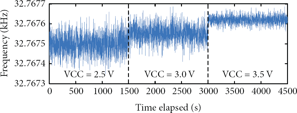
Clock frequency measurement.

Compared with the temperature measurements obtained by sensors, the voltage measurements contain considerably lower noise with a higher precision and are thus more conducive to clock skew estimation. In addition, the voltage value can be directly obtained by nodes without any extra hardware or sensor support, thus consuming less energy than EACS [7] and TCTS [8]. To provide a tradeoff between synchronization accuracy and energy efficiency, we further propose a dynamic resynchronization scheme, which can adjust the resynchronization interval dynamically based on the observed error accumulation. Our solution is generally applicable to most existing networks and is particularly suitable for networks where communication gets either lost or severely impacted, since the skew estimation largely relies on local information.

The proposed VATS approach is composed of two core phases: local time maintenance and dynamic resynchronization. These two phases both lean upon a voltage-skew relational table obtained through empirically study. The contributions of this work are summarized as follows.

• (i)

We empirically study the correlation between the voltage and clock skew. Starting from a simple examining in laboratory, our measurement validates that the voltage is able to serve as a viable reference for clock skew estimation.

(ii)

Based on the observation of the skew-voltage experiment, we introduce a novel voltage-aware time synchronization scheme for autonomously skew estimation, which substantially improves the clock accuracy and reduces the energy consumption.

(iii)

We further propose a dynamic resynchronization scheme for adaptive clock calibration, which advances an important step towards system efficiency and flexibility.

(iv)

Simulation results illustrate the superior performance of the proposed method in terms of calculation accuracy, robustness, and reduced timestamp exchanges for energy saving.

The rest of the paper is organized as follows. Section 2 summarizes the related work. In Section 3 we introduce the preliminary information of this paper. Section 4 presents our initial empirical measurement study that motivates this work. The major design of our two-phase voltage-aware clock time synchronization protocol is given in Section 5. Section 6 shows the performance evaluation results obtained from extensive simulations. Finally, Section 7 concludes the whole paper.

2. Related work

Recent years have witnessed the emergence of many clock synchronization schemes designed for wireless sensor networks. These protocols have their own benefits, respectively, as well as limitations. Previous researches mostly focus on combating the nondeterminism along the critical path of wireless communication. RBS [5] eliminates the send and access delay by applying a receiver-receiver scheme, and it is also possible to remove the receive time uncertainty with minimal OS modifications. While TPSN [4] proposed a “pair-wise handshake” model to successfully estimate the unknown propagation delay, it, meanwhile, eliminates the same three delays as in RBS through MAC layer time-stamping scheme. FTSP [6] promotes the precision by the use of multiple MAC layer time-stamping and comprehensive error compensation. However, compared with the nondeterminism along the critical path, unstability of the oscillator frequency becomes the inherent cause for clock desynchronization and makes it unreasonable to carry out clock synchronization using existing schemes.

To tackle the problem mentioned above, the researchers shift their focus on studying the fundamentals of clock uncertain to achieve higher performance precision. Initially, constant-skew clock model [9, 10] is applied to describe the clock skew, and linear regression [4, 5, 11] is utilized to estimate the clock skew. Considering the strong assumption of constant-skew model, many designs employ the bounded skew model [12, 13] to achieve higher precision. However, clock frequency often influenced by voltage, temperature [7, 8, 14], and so forth, so constant model and bounded model are not applicable here. References [7, 14, 15] use a hybrid two-model system to describe the clock skew and tackle the model uncertainty problem with complex Kalman filtering.

On the other hand, an emerging type of solutions has been recently proposed, which makes use of external measurement to assist skew estimation. Some of them tune to certain external signal source as common time reference. Typical examples are Wi-Fi [16], power lines [17], FM radio [18], and fluorescent lighting [19]. Other solutions, such as [7, 8], utilize the correlation between clock skew and environmental data to track the clock skew. However, most of these schemes introduce extra hardware [16–18] to capture periodical signals, or some of them need to collect environmental information [7, 8, 19], which may introduce extra overhead (in the situation that the collected environmental information is useless for the application). Reference [14] takes voltage into consideration when estimating clock skew; however, it fails to work out the correlation between clock skew and the voltage.

Different from the aforementioned schemes, our design explores the voltage supply compensated scheme to estimate the clock skew. The voltage value can be straightforwardly gained by nodes without any extra hardware or sensors support, which distinctly reduces the energy consumption. In addition, the voltage data contain considerably lower noise than the environmental data measurement.

3. Preliminary

For presentation clarity, we first define the important terms we use to describe clock behavior in this paper.

3.1. Clock Offset versus Clock Skew

Clock. The device used to measure time is called clock. Clock consists of a periodic signal source and a counter to record the number of periods from a starting point. We denote the reading of clock A at real time t as $C_A(t)$ .

Clock Offset. Due to the combination of factors in fabrication and the working environment, the periodic signal of different clocks output frequencies with small offsets from the desired value. As a result, the clock reading is different from the real value. Clock offset is used to describe the difference between the reading of two or more different nodes. We denote the clock offset of clock A relative to clock B at real time t is as ${\theta }_{A,B}(t)$ :

$$\begin{array}{cc}& {\theta }_{A,B}\left(t\right)=C_A\left(t\right)-C_B\left(t\right).\end{array}$$

(1)

Clock Skew. It is the slope of the change in clock offset, and it reflects the frequency difference of two or more different nodes, which is the inherent cause for clock desynchronization. We denote the clock skew of clock A relative to clock B at real time t as

$$\begin{array}{cc}& {\alpha }_{A,B}\left(t\right)=\frac{d{\theta }_{A,B}\left(t\right)}{dt}=\frac{{\theta }_{A,B}\left(t+\zeta \left(t\right)\right)-{\theta }_{A,B}\left(t\right)}{\zeta \left(t\right)},\end{array}$$

(2)

where ζ is the interval measured by real time.

3.2. Skew Model

In the ideal situation, the clock offset is a constant value, which means that the clock skew is 0. However, the frequency of an oscillator fluctuates over time due to the changes in supply voltage, temperature, and so forth. The instability of clock frequency leads to the variation of clock skew. Fortunately, the clock skew is not an arbitrary value, and it can be described by different clock skew models:

Constant Skew Model. The clock skew is assumed to be constant, and the variation of the skew can be included into the processing noise, which can be considered as crystal jitter (shown in (5)). This is reasonable if the required precision is low:

$$\begin{array}{cc}& \alpha \left(t\right)=\alpha +\Phi \left(t\right),\end{array}$$

(3)

where $\Phi (t)$ is the processing noise.

Bounded Skew Model. The deviation of the clock skew from the ideal value ( $\alpha (t)=\mathrm{0}$ ) is assumed to be bounded. We denote the upper bound of clock skew as ${\alpha }_{\max }$ , and the corresponding lower bound as ${\alpha }_{\min }$ . So the bounded skew model can be described as

$$\begin{array}{cc}& {\alpha }_{\min }<\alpha \left(t\right)<{\alpha }_{\max }\end{array}$$

(4)

Constant-Rate Skew Model. The variation of skew is assumed to be a constant rate process. We denote the changing rate of a clock skew as ρ, so the constant-rate skew model can be described as

$$\begin{array}{cc}& \alpha \left(t\right)=\alpha \left(t-\tau \right)+\tau \rho +\Phi \left(t\right).\end{array}$$

(5)

This assumption is reasonable if the skew is influenced only by gradually changing conditions such as voltage supply or temperature.

3.3. Timestamps Exchange

Considering a simple skew estimation case with two nodes, let a node sends timestamps to the other node periodically about its local time reading. In Figure 2, we illustrate two synchronization periods. Node A sends timestamps at times $t_A(t_{\mathrm{0}})$ and $t_A(t_{\mathrm{1}})$ and then node B obtained the two messages at $t_B(t_0^{\prime })$ and $t_B(t_1^{\prime })$ . As a result, node B can acquire the following two pieces of information. (i) The time elapsed at node A is $\Delta t=t_A(t_{\mathrm{1}})-t_A(t_{\mathrm{0}})$ and (ii) the drift offset δ between two nodes during the interval is

$$\begin{array}{cc}& \widehat{\delta }=\left(t_A\left(t_{\mathrm{1}}\right)-t_A\left(t_{\mathrm{0}}\right)\right)-\left(t_B\left(t_1^{\prime }\right)-t_B\left(t_0^{\prime }\right)\right).\end{array}$$

(6)

Thus the observed clock skew then can be expressed as

$$\begin{array}{l}{\widehat{\alpha }}_{A,B}\left(t_{\mathrm{0}}\right)=\frac{{\theta }_{A,B}\left(t_{\mathrm{1}}\right)-{\theta }_{A,B}\left(t_{\mathrm{0}}\right)}{t_B\left(t_1^{\prime }\right)-t_B\left(t_0^{\prime }\right)}\\ \hspace{1em}\hspace{1em}\hspace{1em}=\frac{\left(t_A\left(t_{\mathrm{1}}\right)-t_A\left(t_{\mathrm{0}}\right)\right)-\left(t_B\left(t_1^{\prime }\right)-t_B\left(t_0^{\prime }\right)\right)}{t_B\left(t_1^{\prime }\right)-t_B\left(t_0^{\prime }\right)}.\end{array}$$

(7)

There are several sources that cause errors in skew estimation when timestamps exchange, for example, the delay along the critical path of message delivery, the message construction delay at the sender side, and the processing delay at the receiver side. We treat those uncertain errors as a random variable d, and it is assumed to be white Gaussian noise as

$$\begin{array}{cc}& d~N\left({\mu }_d,{\sigma }_d^{\mathrm{2}}\right).\end{array}$$

(8)

Therefore we can rewrite the observed clock skew as

$$\begin{array}{cc}& {\widehat{\alpha }}_{A,B}\left(t_{\mathrm{0}}\right)={\alpha }_{A,B}\left(t_{\mathrm{0}}\right)+\frac{d_{\mathrm{1}}-d_{\mathrm{0}}}{\Delta t},\end{array}$$

(9)

where $d_{\mathrm{0}}$ and $d_{\mathrm{1}}$ are uncertain errors of messages $t_{\mathrm{0}}$ and $t_{\mathrm{1}}$ , respectively, and ${\alpha }_{A,B}(t_{\mathrm{0}})$ is the real value of clock skew of clock A relative to clock B at time $t_{\mathrm{0}}$ . We can conclude that ${\widehat{\alpha }}_{A,B}(t_{\mathrm{0}})$ is an unbiased estimation for ${\alpha }_{A,B}(t_{\mathrm{0}})$ with error variance $\mathrm{2}{\sigma }_d^{\mathrm{2}}/\Delta t^{\mathrm{2}}$ . In this manner, if we use a uniform sending interval where $\Delta t=T$ , the clock skew of node A at ith sample can be written as

$$\begin{array}{cc}& {\alpha }_{A,B}\left[i\right]=\frac{(t_A[i+\mathrm{1}]-t_A\left[i\right])-\left(t_B\left[i+\mathrm{1}\right]-t_B\left[i\right]\right)}{T}\end{array}$$

(10)

thus we can obtain a series of clock skew measurements $\{{\alpha }_{A,B}[\mathrm{0}],{\alpha }_{A,B}[\mathrm{1}],{\alpha }_{A,B}[\mathrm{2}],\dots ,{\alpha }_{A,B}[n]\}$ .

Figure 2

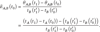
Synchronization between two nodes.

4. Empirical Measurement Study

To accurately estimate the clock skew, we first investigate its property from measurement results. The measurement focuses on evaluating the correlation between the clock skew and the voltage supply value. The clock skew is measured by the timestamps exchange as explained in Section 3.3.

4.1. Measurement Setting

We use a laptop (IBM ThinkPad-X61) as a reference device and assume that its clock reading is the real time. A node is set to send timestamps containing the voltage value at a constant internal as shown in Figure 3. The sending interval is set to one second for simplicity. Another node, which is connected to the laptop, receives the timestamps from the sender and offers an interrupt signal to the laptop as soon as the timestamp arrives. Hence, we can use these messages to obtain the clock skew measurement as discussed in Section 3.3. To avoid the buffer jitter, when a serial port event interrupt is triggered, the laptop will read the system time right away and then process the timestamp immediately.

Figure 3

The experimental equipment: a node for sending timestamps, a node with temperature sensor, and a stabilized voltage supply.

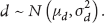
Since a precise control of voltage supply is required in this experiment, the node is driven by a stabilized voltage supply instead of fresh batteries. In this measurement, the voltage value is set to vary from 2.5 V to 5.5 V, with the step of 0.5 V. As we mentioned in Section 3.3, the delay along the critical path of message delivery can be considered as white Gaussian noise with the error variance $\mathrm{2}{\sigma }_d^{\mathrm{2}}/\Delta t^{\mathrm{2}}$ . To minimize this error, we collected more than 10000 pieces of skew measurements for each voltage supply. Besides, to remove the noisy data caused by the temperature variation, another node which connected to a temperature sensor is used to monitor the temperature of the laboratory as shown in Figure 3. If the temperature is beyond a certain range, the collected data will be removed. We put the three nodes and the laptop together in the laboratory environments: a closed temperature controlled building with air conditional.

4.2. Measurement Result and Analysis

The measurement result is show in Figure 4. From the figure, we can observe that, despite the inherent clock skew of the three nodes different from each other, the clock skew of these nodes presents a similar increase tendency when the voltage decreases. For instance, as the voltage descends from 5.5 V to 2.5 V, the clock skew of node3 increases from 9.15 ppm to 15.26 ppm, which means that the clock skew of node3 increases at a speed of 2 ppm/v. In other words, the effect of the voltage change is significant and cannot be ignored. To reveal the correlation, we calculate the Pearson product moment correlation coefficient ( ${\rho }_{X,Y}=E[(X-u_X)(Y-u_X)]/({\sigma }_X{\sigma }_Y)$ ) of the clock skew and voltage measurement. The coefficient result is −0.9767, indicating that the voltage supply and clock skew are indeed highly correlated.

Figure 4

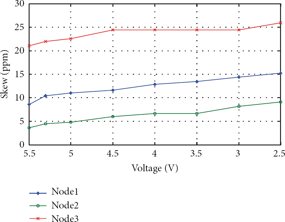
Experiment on voltage and clock skew. In the figure, despite the natural clock skew of the three nodes different from each other, the clock skew of these nodes presents a similar increase tendency as the voltage decrease, which is called “stair phenomenon.”

A more important observation is that, in Figure 4, the correlation between the clock skew and the corresponding voltage exhibits a characteristic “stair phenomenon.” Take, for instance, the changing style of node2. During the period when the voltage decreases from 4.5 V to 3.0 V, the change of clock skew is marginal, and the constant clock skew model discussed in Section 3.2 is compatible to describe it. However, when the voltage decreases from 5.5 V to 4.5 V, the increase of clock skew is comparatively apparent, and thus we can use the constant-rate skew model shown in Section 3.2 to characterize the change of clock skew. We refer to the period when the clock skew increases visibly as the “increase period,” and the period when the clock skew is almost constant as the “stable period.” The observed “stair phenomenon” demonstrates that the clock skew exhibits a hybrid change pattern.

In short, we summarize the conclusion as follows.

• (i)

The clock skew is sensitive to the voltage supply due to the low-cost design of the oscillator; thus, the voltage supply should be taken into consideration for the clock synchronization scheme.

(ii)

The clock skew and the voltage are indeed highly correlated, and this correlation can be used to assist the clock skew estimation.

(iii)

Different clocks exhibit different clock skew change patterns with respect to voltages.

(iv)

Under the influence of the voltage supply, the clock skew presents multiple changing patterns.

5. Two-Phase Voltage-Aware Time Synchronization

In this section, first of all, we first introduce the basic idea of our two-phase voltage-aware time synchronization scheme (VATS) and then give details of the design.

5.1. Overview

The target of VATS is to ensure local time consistent among different nodes. In Section 3, we have stated that the difference between two nodes is referred to as clock offset—the accumulation of clock skew. Clock offset evolves as

$$\begin{array}{cc}& \theta \left(t_i+t\right)=\theta \left(t_i\right)+{{\displaystyle \int }}_{t_i}^{t_i+t}‍{\alpha }_A\left(t\right)dt,\end{array}$$

(11)

where ${\alpha }_A(t)$ is the instant skew of clock A at time t. Considering the accumulation characteristics of clock skew, VATS should calibrate the clock in time to minimize the negative impact of skew and thus prolong the clock resynchronization period. As discussed in Section 4, clock skew is highly correlated to the voltage supply: thus, we can autonomously estimate and compensate the clock skew by referring to the voltage value. Ideally, we have ${\alpha }_A(t)=f_A(V_t)$ , where $f_A(\cdots )$ indicates the function of the voltage supply of node A to clock skew. So (11) can be rephrased as

$$\begin{array}{cc}& \theta \left(t_i+t\right)=\theta \left(t_i\right)+{{\displaystyle \int }}_{t_i}^{t_i+t}‍f_A\left(V_t\right)dt.\end{array}$$

(12)

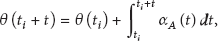
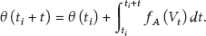
Equation (12) essentially indicated that, by continuously estimating the clock skew, the local clock can be precisely maintained. As a matter of fact, the variance of clock skew is limited within a short period of time and the voltage supply does not change very quickly during the period. Hence, instead of continuously measuring the clock skew, we compensate the local clock by using the native clock and estimated clock skew. To further guarantee the accuracy of such a prediction, we configure the clock calibration in a periodical fashion, as depicted in Figure 5.

Figure 5

Calibration period of VATS.

However, as unveiled in existing works [20], the clock skew and offset estimation often contain varieties of noises. These noises may lead to the accumulation of synchronization error; thus, a periodic resynchronization with the reference node by timestamps exchange is necessary. We introduce a dynamic resynchronization scheme to restrict the total amount of the synchronization error.

In Figure 5, we illustrate two calibration periods. During calibration 1 (blue area), the node estimates the clock skew ${\alpha }_A(t_{\mathrm{1}})$ as ${\widehat{\alpha }}_A(t_{\mathrm{1}})$ at time $t_{\mathrm{1}}$ . After a dormant period continues a fixed duration of $\Delta t$ , the node relies on ${\widehat{\alpha }}_A(t_{\mathrm{1}})$ to calculate the clock offset ${\widehat{\theta }}_A(t_{\mathrm{1}}+\Delta t)$ and update its local time (red area). Note that the clock skew is considered to be constant during the calibration interval. At the end of the calibration period, if a resynchronization is triggered (the time has come for the resynchronization), the node exchange timestamps with the reference (green area). Figure 6 depicts the overview of VATS. There exist three major components in it: clock skew table, local time maintenance, and dynamic resynchronization scheme. The local time maintenance component and the dynamic resynchronization scheme are all based on the reading of the clock skew table.

Figure 6

Overview of VATS.

5.2. Clock Skew Table

In order to compensate the clock skew autonomously, a clock skew table containing clock skew with respect to voltage for each node is required. The table is established based on the training dataset which is obtained from the measurement result in Section 4. This is conducted offline, before the deployment. As discussed in Section 4, different pairs of clocks exhibit different clock skew change patterns with respect to voltage, so the skew table stored in different nodes is independent. It is to note that, in order to retain a common time in the whole network, the table for each node must refer to the same reference.

5.3. Local Time Maintenance

Skew detection serves as the first step towards local time maintenance since the clock offset results from the accumulation of the skew. In our VATS scheme, the clock skew is estimated by using the current voltage supply value and the clock skew table. The obtained voltage of node A in the ith calibration period can be noted as $V_A(t_i)$ . As a result, the estimated clock skew which is obtained referring to the clock skew table can be written as

$$\begin{array}{cc}& {\widehat{\alpha }}_A\left(t_i\right)=\text{Table}\left(V_A\left(t_i\right)\right).\end{array}$$

(13)

Since the clock skew table is course-grained, for most voltage value, there is no corresponding entrance in the clock skew table. Hence, we use a linear approximation to obtain the clock skew based on the nearest two entrances when the table entry is missing:

$$\begin{array}{cc}& {\widehat{\alpha }}_A\left(t_i\right)=\frac{V_A\left(t_i\right)-V_l}{V_h-V_l}\left({\alpha }_h-{\alpha }_l\right)+{\alpha }_l,\end{array}$$

(14)

where $V_h$ and $V_l$ are the nearest two entrances, and we have $V_l<V_A(t_i)<V_h$ . ${\alpha }_h$ and ${\alpha }_l$ are the corresponding clock skew of $V_h$ and $V_l$ . It is clear that table look-up introduces error in skew estimation, and we denote it as $\omega (t_i)$ , so the estimated clock skew can be rephrased as

$$\begin{array}{cc}& {\widehat{\alpha }}_A\left(t_i\right)={\alpha }_A\left(t_i\right)+\omega \left(t_i\right).\end{array}$$

(15)

After the clock skew has been updated as ${\widehat{\alpha }}_A(t_i)$ , the local time afterward can be predicted by using such a new clock skew till the next calibration period. To maintain an accurate local time, in addition to the calibration, we also need to correct the offset accumulated between two consecutive calibrations. We denote ${\widehat{\theta }}_A(t_i+\Delta t)$ as the estimated clock offset of node A in the ith calibration period. Here we assume that the clock skew does not change during a period since the voltage supply does not change very quickly. So we can update the offset as

$$\begin{array}{cc}& {\widehat{\theta }}_A\left(t_i+\Delta t\right)={\widehat{\theta }}_A\left(t_{i-\mathrm{1}}+\Delta t\right)+\Delta t·{\widehat{\alpha }}_A\left(t_i\right).\end{array}$$

(16)

If the clock offset exceeds a given threshold (we call it compensation threshold), we conduct the compensation to the local clock as

$$\begin{array}{cc}& C_A\left(i\right)=C_A\left(i\right)+{\widehat{\theta }}_A\left(t_i+\Delta t\right).\end{array}$$

(17)

5.4. Dynamic Resynchronization Interval Adjustment Scheme

To eliminate the accumulation of synchronization error, a periodic resynchronization with the reference node by timestamp exchange is necessary. Given the resource-constrained characteristic of the WSNs, a tradeoff between accuracy and communication cost is required. We now provide a dynamic resynchronization interval adjustment scheme, in which the resynchronization interval can be controlled through the parameters μ and λ.

(1) Error Controlling Factor Lambda. We first introduce a synchronization error controlling factor μ to restrict the total amount of synchronization error accumulated between two resynchronizations. Suppose the error detected at the last resynchronization period in the ith timestamps exchange is $\text{er}{\text{r}}_i$ and the resynchronization interval length between the ith and the (i+1)th resynchronization is $d_i$ . Then, the next resynchronization interval $d_{i+\mathrm{1}}$ in VATS can be predicted as

$$\begin{array}{cc}& d_{i+\mathrm{1}}=d_i·\frac{\mu }{\left|\text{er}{\text{r}}_{i+1}\right|}.\end{array}$$

(18)

Initially, $d_{\mathrm{0}}$ is set to be 20 min. As shown in (18), if the synchronization error rapidly accumulates, the resynchronization interval should be shorter to eliminate the error in time, and vise versa. Such customization is significant because in practice it is not desirable to provide frequent re-synchronization if the synchronization error is relatively small.

(2) Regulatory Factor Lambda. However, the abovementioned method still needs to be sophisticated. As we have discussed in Section 4, the clock exhibits multiple skew changing pattern with respect to its current voltage, and we will explain next that this phenomenon causes the error accumulating rate difference during different voltage range. Thus the resynchronization interval should also be adaptive to the multiple changing pattern of clock skew. We give the following analysis about it.

As mentioned in Section 5.3, the error introduced by skew estimation is mainly caused by the linear approximation which we used when the table entry is missing. Thus, we have

$$\begin{array}{cc}& \omega \left(t_i\right)=\alpha \left(t_i\right)-\widehat{\alpha }\left(t_i\right),\end{array}$$

(19)

where $\alpha (t_i)$ is the actual clock skew at time $t_i$ and $\widehat{\alpha }(t_i)$ is the estimated value got through the linear approximation. The maximal value of $\omega (t_i)$ is related to the changing rate of clock skew at time $t_i$ , as shown in Figure 7.

Figure 7

Error analysis of the “table look-up.” The estimated value is marked as the blue solid line, and the true value is marked as the blue dashed line.

Figure 7 shows the variation trend of the clock skew of node3 related to the changing voltage with a variation range from 5.5 V to 2.5 V. We take the change between 5.0 V and 4.5 V, for instance, to explain the effect of the changing rate of clock skew on $\omega (t_i)$ . As shown in the subpicture of Figure 7, the assumed true value of clock skew ${\alpha }_A(t_i)$ is marked as the blue dashed line, the estimated clock skew ${\widehat{\alpha }}_A(t_i)$ obtained from (14) (In this instance, $V_h$ is 5 V, and $V_l$ is 4.5 V. The corresponding ${\alpha }_h$ and ${\alpha }_l$ are depicted in Figure 7 as points a and b) is marked as the blue solid line. Therefore, ${\widehat{\alpha }}_A(t_i)$ could have offset error from its true value ${\alpha }_A(t_i)$ as depicted in the figure. We assume that

$$\begin{array}{cc}& {\alpha }_h<{\alpha }_A\left(t_i\right)<{\alpha }_l.\end{array}$$

(20)

Thus the maximal value of $\omega (t_i)$ is

$$\begin{array}{cc}& {\omega }_{\max }\left(t_i\right)=\max \left\{{\widehat{\alpha }}_A\left(t_i\right)-{\alpha }_h,{\alpha }_l-{\widehat{\alpha }}_A\left(t_i\right)\right\}.\end{array}$$

(21)

It is clear that ${\omega }_{\max }(t_i)$ is proportionate to ${\alpha }_h-{\alpha }_h$ as shown in Figure 7. In other words, a relatively marked variation of clock skew leads to a larger synchronization error. Based on this observation, a regulatory factor λ should be introduced in the interval adjustment scheme, in order that the resynchronization interval adjustment manner during the “increase period” (the shadow areas in Figure 7) is different from that during the “stable period.” Thus the resynchronization interval can be rewritten as

$$\begin{array}{cc}& d_{i+\mathrm{1}}=d_i·\frac{\mu ·\lambda }{\left|\text{er}{\text{r}}_{i+1}\right|},\end{array}$$

(22)

where μ is set to be 15 native clock ticks initially, and each native clock tick corresponds to 30.515 us.

λ in Stable Period. The clock skew increases sluggishly in stable duration. Thus the synchronization error introduced by linear approximation is considered negligible compared with the increase duration. We set $\lambda =\mathrm{1}$ in this duration.

λ in Increase Period. Since the clock skew increases rapidly in this duration, the synchronization error introduced by linear approximation is considerably larger. Thus we set that

$$\begin{array}{cc}& \lambda =\frac{V_h-V_l}{{\alpha }_h-{\alpha }_l},\end{array}$$

(23)

where $({\alpha }_h-{\alpha }_l)/(V_h-V_l)$ is the increase rate of clock skew. Equation (23) indicates that a faster increase clock skew leads to a larger λ, which shortens the resynchronization period to eliminate the error in time as shown in (22), and vise versa. It is noteworthy that a threshold (such as 5 min) should be set to prevent an excessively short resynchronization interval, because too frequent clock resynchronization may introduce high communication overhead.

In simple terms, we can summarize the following.

• (i)

The parameter μ can be seen as the required precision, which is used to restrict the unbounded accumulation of synchronization error.

(ii)

The parameter λ is set to adjust the resynchronization interval, in order that the resynchronization interval is adaptive to the multiple changing pattern of the clock skew.

We list operations in our VATS scheme as Algorithm 1.

Algorithm 1: Voltage-aware time synchronization.

(1)    INPUT

(2)    $T_{\text{cs}}$ : Clock skew table with respect to voltage.

(3)   μ: The re-synchronization threshold

(4)   N: The number of periods

(5)   τ: local clock tick unit

(6)   Start

(7)   Initialize the clock offset $\theta (\mathrm{0})=\mathrm{0}$

(8)   Initialize the synchronization error $error(\mathrm{0})=\mathrm{0}$

(9)   for   $i=1$ to N  do

(10)   In Phase I: Local time maintenance;

(11)   Obtain the current voltage supply $V(i)$

(12)   if  exist $V=V(i)$ in the skew table and the corresponding skew is α  then

(13)     $\alpha (i)=\alpha$ ;

(14)   else

(15)    In $T_{\text{cs}}$ , find the largest $V_l$ and the smallest $V_h$ and the corresponding skew ${\alpha }_l$ and ${\alpha }_h$ ;

(16)     $\alpha (i)=\frac{\widehat{V}(i)-V_l}{V_h-V_l}({\alpha }_h-{\alpha }_l)+{\alpha }_l$ ;

(17)   end if

(18)    $\theta (i)=\theta (i-\mathrm{1})+\mathrm{\Delta }t·\alpha (i)$ ;

(19)   if   $\theta (i)>\mu /\mathrm{2}$   then

(20)    $C(i)=C(i)+\theta (i)$ ;

(21)    $\theta (i)=\mathrm{0}$ ;

(22)  end if

(23)  In Phase II: Dynamic interval adjustment;

(24)  if Time out for re-synchronization then

(25)   Exchange timedtamps with reference node;

(26)   if   $V(i)$ in the stable duration then

(27)     $\lambda =\mathrm{1}$

(28)   else

(29)     $\lambda =\frac{V_h-V_l}{{\alpha }_h-{\alpha }_l}$

(30)   end if

(31)   Set the next re-synchronization interval as $d_{i+\mathrm{1}}=d_i·((\mu ·\lambda )/(\left|er{r}_{i+\mathrm{1}}\right|))$

(32)  end if

(33) end for

The code between lines 10–22 describes the local time maintenance phase, which estimates the clock skew and the offset and then compensates the local clock. The code between lines 23–37 describes the dynamic resynchronization phase.

Discussions. To address the challenges of time synchronization in WSNs, first, the clock skew estimation is referring to the nodes' current voltage supply value in VATS; thus, the effect of voltage supply change is removed. Second, the clock skew is compensated appropriately, so the resynchronization period can be substantially prolonged. Given that the communication energy accounts for a major proportion of the energy consumption in WSNs, using our VATS scheme, the overall energy consumption is much less. Third, since our VATS scheme is independent of the network message exchange, time synchronization can be retained even when the network is temporarily disconnected. Such characteristics particularly suit various mobility-enabled scenarios. Besides, this characteristic removes the error accumulation caused by “hop by hop” timestamps exchange.

6. Performance Evaluation and Discussion

Extensive simulations have been conducted to evaluate the performance of VATS. The simulations focus on verifying the following three properties: (i) accurate skew estimation, (ii) robustness, and (iii) long resynchronization period.

6.1. Simulation Setting

We generate the simulation data based on the measurement results of node1, node2, and node3 in Section 4. In the simulation, the voltage varied from 3.5 V to 2.5 V as shown in Figure 8. The corresponding clock skew of the three nodes varied from 13.43 ppm to 15.26 ppm, 36.62 ppm to 39.06 ppm, and 24.42 ppm to 25.94 ppm, respectively, according to the measurement result. The measurement noises followed a Gaussian distribution. We used a set of training data to obtain the table of clock skew compensation with respect to voltage.

Figure 8

The changing voltage supply value, which simulates the power depletion of the fresh batteries.

The reason why we choose the interval of 3.5 V to 2.5 V is that the skew change pattern of the three nodes in this interval is diverse from each other. Thus the difference of clock skew estimation accuracy in different skew change pattern can be observed.

6.2. Accuracy

One of the main advantages of our VATS scheme is that it exploits the relationship of clock skew and voltage to estimate and calibrate the clock skew, which guarantees the skew estimation precision during the resynchronization interval.

Figure 9 shows the skew estimation result of the three nodes. From the figure, we can observe that the estimation results (the red line) of the three nodes are all close to the real values (the yellow line), even though the clock measurements (the dots) contain severe noise. This is because we can estimate the clock skew using voltage estimation, so the negative impact of voltage change is minimized. From the figure, the estimation errors are obvious during partial stage. For node1, during the period that the voltage changes from 3.2 V to 3 V (2000 to 2800 (100 s)), the estimation error appears to be more obvious than other periods. For node3, the estimation error increases during the period that the voltage changes from 3 V to 2.5 V. It is remarkable since the change in estimation error during this period is markedly compared to the period that the voltage changes from 3.5 V to 3 V, during which the estimation results and the real values coincide with each other.

Figure 9

The clock skew estimation performance. We can clearly see that the estimation results of the three nodes are all close to the real values even though the clock measurements contain severe noise. The performance of VATS is extremely high.

To further evaluate the estimation error, the square error of the three nodes is shown in Figure 10. The result shows that, despite the accuracy of the three nodes gap big (it is caused by fabrication process or other individual factors), the tendency of the accuracy has the common obvious temporality, which is consistent with the estimation results and the real values shown in Figure 9. The sudden increase of the estimation error is considered prompted by the speed increases of clock skew, which is explained in Section 5.4. From Figure 4, we can observe that, for node3, the clock skew accelerates from 3 V to 3.5 V; as a result, Figure 10 exhibits a sudden error increase during 3000 to 3400 (100 s) of node3. The other two nodes exhibit the same pattern. The sudden increase of skew estimation increase can be restricted by the “dynamic interval adjustment scheme” introduced in Section 5.4.

Figure 10

The clock skew estimation variance. The tendency of the accuracy of node1, node2, and node3 has the common obvious temporality, which is consistent with the estimation results and the real values shown in Figure 9.

From statistics, we find that the average error (the solid red line) for every 100-time slot (100 s) keeps less than $\mathrm{0.05}$  ppm² all the time and it is smaller than 0.02 ppm² for over 80% of time. The maximum logic time (the dotted green line) error is also well controlled. Statistics show that the maximum error is always smaller than 0.09 ppm² and it is less than 0.05 ppm² most time. Figure 10 indicates that clock skew can be precisely estimated by VATS.

6.3. Robustness

Another advantage of VATS over the TETS schemes is in scenarios where the network is temporarily disconnected. Examples of such scenarios are atrocious environmental conditions (such as blizzard and torrential rain which may damage the antenna), mobility, or secrecy actions where radio silence is necessary. In these scenarios, VATS can still obtain the desired voltage values for clock skew estimation, and the calibration mainly relies on the voltage value. In contrast, the TETS schemes can only rely on the clock skew estimated by the last timestamp exchange.

Figure 11 compares the clock offset of VATS (the red line) with the TETS schemes (the blue line) when the network is disconnected. The result shows that, at the initial stage (0–1000 s), the performances of VATS and TETS schemes are almost parallel. However, after the voltage starts to change significantly from the initial voltage, the TETS scheme starts to lose accuracy since the gap between the current voltage and the voltage when the last clock skew estimated by the TETS scheme starts to increase, while TCTS can keep its accuracy at a very precise level. Over the 4 days where no timestamp exchange occurs, our VATS scheme only accumulates less than 0.03 s of time synchronization error.

Figure 11

Illustration of what happens if time synchronization is stopped. We can clearly see how TETS schemes performance worsens once the network is disconnected, whereas VATS keeps the synchronization accuracy at a much higher level.

On the other hand, we noted that the compensated clock offset is in a zigzag style as shown in the subfigure. This is because the clock offset compensation is based on the compensation threshold. Therefore, only the offset accumulated to a certain threshold can be compensated using (17) as discussed in Section 5.3.

6.4. Period

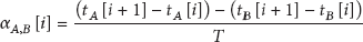
To understand the resynchronization period of our VATS scheme, we evaluate the VATS under different error controlling factor μ. We choose five different error controlling factors to be 5, 10, 15, 25, and 30 native clock ticks. For each μ, the experiment lasts 96 hours. When the experiment terminates, we calculate the average length of the resynchronization interval and the timestamp exchange frequency under each controlling factor. The statistical result is shown in Figure 12. It is obvious that the average length of the resynchronization interval lengthened as the controlling factor increases; meanwhile, the timestamp exchange frequency is reduced. That is because a larger μ indicates a looser requirement of synchronization precision; thus a long resynchronization period is adequate.

Figure 12

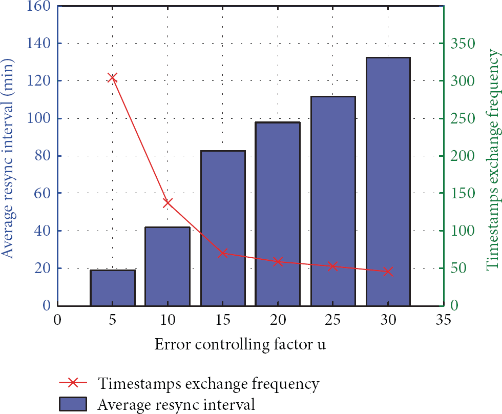
This graph shows the average resynchronization interval and the timestamps exchange frequency under different error controlling factors. The resynchronization interval rapidly lengthened as the error controlling factor increased and thus save power and communication overhead.

We can also observe from the figure that the resynchronization interval is usually longer than 18 min even the error controlling factor is 5 native clock ticks, while that for TETS schemes is less than 150 s. In other words, using TATS, the synchronization communication cost is reduced by an order of magnitude, which is highly desired for power-constrained wireless sensor networks.

7. Conclusion and Further Discussion

In this paper, we have proposed a novel voltage-aware time synchronization (VATS) scheme for wireless sensor networks. The VATS scheme is based on the fact that clock skew is highly correlated to the voltage supply. By using the relationship between clock skew and voltage supply, the clock that is updated only relies on the local information before the clock resynchronization is triggered, which prolongs the resynchronization period in significant measure. This improvement achieves the overall network energy saving since fewer timestamps exchange is needed, which is significant for the power-constrained wireless sensor networks. To remove the accumulated error in skew estimation, we introduce a dynamic resynchronization. This scheme considers both the accuracy and the cost. In addition, our VATS scheme is also applicable to the scenarios where the network is temporarily disconnected which improves the robustness of the whole networks.

In this paper, we adopt a widely used assumption that the temperature or other environmental parameters are constant and in a most suitable condition. This assumption is somewhat unrealistic in some practical settings. In our future research, we will investigate the impact of other environment factors (such as temperature, humidity, electromagnetic interference, and vibration) on clock skew which are treated as noise in this work.