Multiobjective Optimization of CRH3 EMU Wheel Profile

Abstract

The wheel-rail wear problems inherent to railway operation have become increasingly prominent and serious, as they have been proven to be the main factors which affect safety, stability of electric multiple units (EMUs), and wheel-rail maintenance cost. The multiobjective optimization model of CN wheel profile proposed in this study was constructed in effort to reduce the wheel wear of CRH3. Reconstruction of the CN profile based on the nonuniform rational B spline (NURBS) curve theory was designed. Twenty vertical coordinates of the CN profile were selected as design variables, the first wheelset mean wear workand the wheel-rail lateral force were employed as the objective functions, and the wheel geometry, maximal contact pressure, and the derailment coefficient were chosen as the constraint conditions. Particle swarm optimization (PSO) was applied to complete the optimization model combined with the vehicle track coupling dynamics model. Analysis results indicated that the optimized CN-Opti profile possesses more favorable, comprehensive, dynamic, and effective characteristics than the traditional CN profile.

1. Introduction

The wheel profile is a crucial parameter of high speed trains, as it determines the hunting stability, curve negotiation performance, wheel and rail wear, derailment coefficient, and other dynamic performance factors [1]. In order to optimize the wheel profile effectively, specific parameters must be iteratively adjusted. To this effect, reasonable parameter design is extremely important.

Currently, there exist several mathematic methods for wheel profile design. (1) The mathematical fitting method for finite discrete points: Shevtsov et al. [2, 3] and others established models by selecting the vertical coordinate of the wheel profile as variables and the rolling radii difference of the wheel as an objective function. Jahed et al. [4] proposed a cubic spline interpolation method to ensure the convexity and monotony of wheel profiles. Liu [5] used the B spline fitting of discrete points to describe the wheel profile and further applied their model in an optimized design based on rolling radii difference. Zhang et al. [6] used the cubic spline of discrete points and maintained the x-coordinate Y for consistency, selecting the y-coordinate Z as a variable for numerical analysis. Choromanski and Zboinski [7] used Chebyshev orthogonal polynomials to describe the wheel profile. (2) The mathematical method, which takes the geometric properties of a point on the wheel profile as variable: Heller and Law [8] established a function for vehicle stability and curve negotiation performance using the tangent and of arc radius at points on the wheel profile as variables. Persson and Iwnicki [9] established a multiobjective optimization model in which design variables are selected as weight sum of the penalty factor plus vehicle dynamics performance, along with a high order derivative of points on the wheel profile, forming a wheel profile description method with fitting for finite arcs. Smith and Kalousek [10] posed a synchronous optimization method for arcing wheel profiles. Cheng et al. [11] established a multiobjective optimization model for the wheel profile with many arcs and centers at different radii as design variables.

Researchers have also selected wheel-rail geometric contact properties as variables to establish objective function and find optimal wheel profile reversely, with relative success. Shen et al. [12, 13] proposed contact angle as a prominent factor in the design of a wheel profile, a novel approach to wheel profile optimization. Constructing wheel profiles using NURBS curve was studied by Liu and He [14], ultimately providing a parametric modeling basis of standard wheel profiles. Further parameters are necessary, however, to fully account for worn wheel profiles as these affect computational efficiency.

Wheel wear is a very important subject for railway administrators. Successful, methodic design of wheel profiles in order to directly reduce wheel wear is a critical research field in this regard. A number of disadvantages exist to make this difficult, however. For example, when a greater number of data points are used to describe a wheel profile, the computational cost is often very high, making the optimization process significantly more difficult. Reasonable mathematic methods and design parameters are extremely important for the optimized design of the wheel profile, but these can be difficult to achieve because most methods currently used possess relevant deficiencies, such as difficult description of high order fitting, issues with local characteristics of the profile curve or smoothness, and large margin of error in multiple arc fittings.

Nonuniform rational B splines, commonly referred to as NURBS [15, 16], have become the de facto industry standard for the representation, design, and data exchange of geometric information processed by computers. NURBS algorithms are quick to use and highly numerically stable [17, 18]. A NURBS curve is used in this paper to describe a wheel profile with few selected data points; then its effectiveness is verified by analysis. A model wheel profile of a CRH3 (China railways high speed) EMU is established with statistics of a worn wheel profile and the convexity and continuity of the profile curve as geometric constraints to reduce mean wheel wear work and wheel/rail lateral force. The PSO algorithm [19] is also used to search for a well-matched wheel/rail profile, so as to effectively reduce wheel wear.

2. Cubic NURBS Curve Model

The wheel profile curve is a special curve which not only requires smoothness, but is also highly dependent on local changing laws of the wear wheel type. Curves generated by NURBS have many advantages, characterized primarily by local modification, unique convexity, and possession of C¹ continuity at the connection points of curves.

2.1. NURBS Definition

The curve's form is as follows:

$p\left(u\right)=\frac{{\sum }_{i=\mathrm{0}}^n{\omega }_i{d}_i{N}_{i,k}\left(u\right)}{{\omega }_i{N}_{i,k}\left(u\right)}$

(1)

in which d _i (i = 0, i, …, n) is the control point and ω _i (ω₀, ω _n > 0, other ω _i ≥ 0) is the corresponding weight factor sequence as related to the control point d _i ; N _{i, k} (u) is the B spline basis function determined by knot vector U = [u₀, u₁, …, u_{n + k + 1}]. The Cox-de Boor recursion formula of the primary functionis

$\begin{array}{c}{N}_{i,\mathrm{0}}\left(u\right)=\left\{\begin{array}{cc}\mathrm{1},\hfill & u\in [u_i,u_{i+\mathrm{1}}]\hfill \\ \mathrm{0},\hfill & u\notin [u_i,u_{i+\mathrm{1}}]\hfill \end{array}\right)\\ N_{i,\mathrm{0}}\left(u\right)=\frac{u-u_i}{u_{i+k}-u_i}{N}_{i,k-\mathrm{1}}\left(u\right)+\frac{u_{i+k+\mathrm{1}}-u}{u_{i+k+\mathrm{1}}-u_{i+\mathrm{1}}}{N}_{i+\mathrm{1},k-\mathrm{1}}\left(u\right).\end{array}$

(2)

The knot vector U = [u₀, u₁, …, u_{n + k + 1}] is determined by the chord length parameterization:

$\begin{array}{c}{u}_{\mathrm{0}}=\mathrm{0},\\ u_i=u_{i-\mathrm{1}}+\left|\Delta p_{i-\mathrm{1}}\right|,\hspace{1em}i=\mathrm{1,2},\dots ,n,\end{array}$

(3)

where |Δp_{i − 1}| is the forward vector integral and Δp _i = p_{i + 1} − p _i is the chord length vector.

2.2. Reverse Algorithm for the Cubic NURBS Control Point

To generate a NURBS curve by the finite data points on a wheel profile, n data points p _i and their n + 2 corresponding weight factors h (i = 0, …, n + 1) are required. Reverse calculation is performed for the control point. Assume that the weight factors of the control point ω _i and of the data point h _i have the following relationship:

$\begin{array}{c}\frac{\mathrm{3}({\omega }_{\mathrm{1}}-{\omega }_{\mathrm{0}})}{u_{\mathrm{4}}-u_{\mathrm{3}}}=h_{\mathrm{1}}=h_{\mathrm{0}}\\ \frac{\mathrm{3}({\omega }_{n+\mathrm{1}}-{\omega }_n)}{u_{n+\mathrm{2}}-u_{n+\mathrm{1}}}=h_n=h_{n+\mathrm{1}};\end{array}$

(4)

n equations can be generated according to the above formula. Targeting the characteristics of the wheel profile curve, two tangent and vector boundary conditions are achieved. Then, d _i of the n + 2 control point can be determined.

2.3. Verification of the Cubic NURBS Curve

Finite data points on the wheel profile are selected, and the cubic NURBS computation method is used to reversely calculate the coordinate and weight factors of the spline curve to establish a universal NURBS method for wheel profile optimization (Figure 1).

Figure 1:

Comparison between cubic NURBS CN curve and original CN curve.

2.3.1. Determination of Data Point

Accurate curve generation requires that the method of selecting data points and the number of data points are very carefully determined. The gradient of the wheel flange varies quite widely, but the gradient of the tread hardly varies, so densely distributed data points at the wheel flange help to precisely describe the wheel flange. The total curve length at x = [1, 120] mm is uniformly divided into N − 1 arcs to obtain N data points, allowing more data points at the wheel flange to be sampled. Notably, relevant advantages of NURBS include its use of finite data points to describe complicated curves, plus how easily adjustments are made in the process. In this paper, three cases are separately compared to the profile curve, divided into 14, 19, and 24 arcs with 15, 20, and 25 data points, respectively, so as to identify the optimum number of data points.

2.3.2. Weight Factor of Data Points

The weight factor of data points potentially indicates their importance in the curve. A large weight factor of certain data point indicates its greater influence on adjacent points and vice versa. There is no previous study for reference on this matter, and the flange is crucial to the wheel profile, so in this study, values are very carefully selected. At the wheel flange x = [15, 40] mm, the weight factor of data points is set to [0.9, 1.0]. At a tread of x = (40, 110] mm, the weight factor of data points is set to [0.6, 0.8]. Weight factor of data points at other parts are set to [0.5, 0.7].

2.3.3. Cubic NURBS Fitting Validation

To validate the method's feasibility, the CN wheel profiles of CRH3 EMUs are selected for fitting design with 15, 20, and 25 data points selected, respectively. To determine the effectiveness of the method, correlation analysis is made between the original profile curve and the cubic NURBS curves. The correlation coefficients COR_CN obtained are shown in Table 1.

Table 1:

Correlation of CN profile before and after NURBS design.

Case	Number of data points N	CORCN
1	15	0.83
2	20	0.93
3	25	0.97

Table 1 indicates that the more the data points are selected, the closer the fitting curve is to the original curve. Comprehensive analysis likewise indicated that selection of 20 data points for the cubic NURBS curve design shows better results in describing CN wheel profiles. Therefore, it is proven feasible to select 20 data points for the fitting of the difference.

The above analysis demonstrably proves that N = 20 data points in the cubic NURBS curve design show optimal results in describing the wheel profile. The major data point p _i , weight factor ω _i , and the control point d _i are reversely calculated as shown in Table 2.

Table 2:

Major parameters for cubic NURBS CN curve.

Data points p i			Weight ω		Control data d i
i	x i	y i	i	ω i	i	x i	y i
1	1.00	−12.99	0	0.5	0	1.00	−10.53
2	4.31	−19.57	1	0.7	1	1.98	−8.02
3	9.29	−24.98	2	0.7	2	2.50	−19.79
4	15.89	−28.06	3	1.0	3	7.42	−23.05
5	23.03	−26.81	4	1.0	4	13.30	−28.37
6	27.41	−21.02	5	1.0	5	21.49	−28.66
7	29.63	−13.99	6	1.0	6	27.26	−22.98
8	33.06	−7.56	7	1.0	7	29.07	−15.79
9	39.40	−3.89	8	1.0	8	31.15	−8.25
10	46.44	−1.66	9	0.8	9	37.93	−4.08
11	53.68	−0.27	10	0.8	10	45.04	−1.91
12	61.00	0.67	11	0.8	11	52.43	−0.38
13	68.36	1.21	12	0.8	12	59.88	0.63
14	75.74	1.52	13	0.8	13	67.38	1.20
15	83.12	1.66	14	0.8	14	74.90	1.51
16	90.50	1.57	15	0.7	15	82.41	1.73
17	97.88	1.63	16	0.7	16	89.9	1.53
18	105.25	1.87	17	0.6	17	97.38	1.59
19	112.63	2.15	18	0.5	18	105.29	1.89
20	120.00	2.62	19	0.5	19	111.33	2.01
			20	0.5	20	120.00	2.62
			21	0.5	21	120.00	2.62

3. Optimization Model for Low-Wear Wheel Profile

The above method has provided a basis for the selection of variables for wheel profile optimization for wear reduction. CRH3 EMU provides an example here for the optimization of a low-wear wheel profile.

3.1. Design Variables

The vertical coordinate y _i (i = 1, 2, …, 20) of the N = 20 data points on the wheel profile is considered the variable. The horizontal coordinates of the data points are shown in Table 2. The NURBS fitting method mentioned above is then applied to generate a wheel profile. Initialization is performed by taking the CN standard profile as a default value to search for an optimized low-wear profile.

3.2. Objective Function

The following objective function is established to reduce wheel wear on the entire railway.

1. Objective function for reduction of wheel wear:

   $\begin{array}{c}{f}_{\mathrm{1}\min }\left(y_i\right)=\frac{\mathrm{1}}{s}{{\displaystyle \int }}_{t_{\mathrm{0}}}^{t_{\mathrm{1}}}\left(W_L\left(t\right)+W_R\left(t\right)\right)dt,\\ W_L\left(t\right)=\frac{\mu }{\mathrm{0.6}}·\frac{T_{xL}{\nu }_{xL}+T_{yL}{\nu }_{yL}}{A},\\ W_R\left(t\right)=\frac{\mu }{\mathrm{0.6}}·\frac{T_{xR}{\nu }_{xR}+T_{yR}{\nu }_{yR}}{A},\end{array}$

   (5)

   where W _L (t) and W _R (t) are the wear work of the left and right wheels of the first wheelset, respectively, and S is the total length of simulated track. T _xL and T _yL are longitudinal and lateral creep force of the left wheel, respectively; T _xR and T _yR are longitudinal and lateral creep force of the right wheel, respectively; ν _xL and ν _yL are longitudinal and lateral creepage of the left wheel, respectively; ν _xR and ν _yR are longitudinal and lateral creepage of the right wheel, respectively. A is the wheel-rail contact area, and μ is a friction coefficient.

2. Objective function for maximum wheel/rail lateral force:

   $f_{\mathrm{2}\min }\left(y_i\right)=\max \left\{\left|Q_L\right|,\left|Q_R\right|\right\}$

   (6)

   in which Q _L , Q _R are wheel/rail lateral forces of both the left and right wheels on the first wheelset that have undergone low-pass filter processing.

3.3. Constraint Function

To make the curve smoother and prevent any singular points, the vertical coordinate statistics, monotony, and convexity of the curve as well as the range of inflection points are selected to be geometric constraints. The maximum wheel/rail contact stress and derailment coefficient are considered constraints as well.

3.3.1. Geometric Constraints for the Wheel Profile Curve

(1) Constraints for the Vertical Coordinate Range of the Data Points. Eight worn wheel profiles of CRH3 EMUs after running 200,000 km along with the CN wheel profile are selected as two boundary conditions of the design variable:

$C_{\text{down}}\left(y_i\right)\le y_i\le C_{\text{up}}\hspace{1em}i\in (\mathrm{1,2},\dots ,\mathrm{20})$

(7)

in which C_down(y _i ), C_up are the respective boundary conditions (the worn profiles and CN profile).

(2) Constraints on Monotonicity of Curve from Wheel Flange to Tread. It is assumed that fitting function for an optimized wheel profile curve is g(y _i ). The constraint on the first derivative of the curve from top wheel flange to tread is

$f\left[g^{\prime }\left(y_i\right)\right]\ge \mathrm{0}\hspace{1em}i\in \left(\mathrm{5},\dots ,\mathrm{20}\right).$

(8)

(3) Constraints on Convexity of Wheel Profile. According to wheel profile statistical analysis, it is assumed that the profile of g(y _i ) has two convexity variations: the concave-convex variation and concave-convex-concave variation.

• Constraints on concave-convex-concave variation:

  $\begin{array}{c}f\left[g^{\mathrm{\prime \prime }}\left(y_i\right)\right]<\mathrm{0},\hspace{1em}\hspace{1em}f\left[g^{\mathrm{\prime \prime }}\left(y_i\right)\right]>\mathrm{0},\\ i\in \left[\left(\mathrm{6,9}\right)\cup \left(\mathrm{13,20}\right)\right].\end{array}$

  (9)

• Constraints on concave-convex variation:

  $\begin{array}{c}f\left[g^{\mathrm{\prime \prime }}\left(y_i\right)\right]<\mathrm{0},\hspace{1em}\hspace{1em}f\left[g^{\mathrm{\prime \prime }}\left(y_i\right)\right]>\mathrm{0},\\ i\in \left(\mathrm{6,9}\right).\end{array}$

  (10)

3.3.2. Constraint on Maximum Wheel/Rail Contact Stress

The constraint on contact stress is

$(P_{\text{CN}\_\text{Opti},\max }-P_{\text{CN},\max })\le \mathrm{0},$

(11)

where P_{CN_Opti, max ⁡} and P_{CN, max ⁡} are the maximum wheel/rail contact stress for both CN-Opti and CN wheel.

3.3.3. Constraint on Derailment Coefficient

According to the Nadal equation, the constraint on vehicle derailment coefficient is

$\begin{array}{c}{f}_d=\left(\frac{Q}{P}\right)\le \frac{\tan {\alpha }_{\mathrm{1}}-{\mu }_{\mathrm{1}}}{\mathrm{1}+{\mu }_{\mathrm{1}}\tan {\alpha }_{\mathrm{1}}},\\ {\left(f_{d,\text{CN}\_\text{Opti}}\right|}_{\max }-{\left(f_{d,\text{CN}}\right|}_{\max }\le \mathrm{0},\end{array}$

(12)

where Q and P are, respectively, lateral and vertical wheel/rail forces. α₁ is the angle of the wheel flange. The max value of derailment coefficient is thus obtained.

4. Vehicle/Track Dynamics Model

Considering the actual running properties of CRH3 EMUs, the Universal Mechanism is used to establish a dynamic model. Statistics of the measured Beijing-Tianjin high-speed railway provide reference data, and a serious wear condition with a small radius is studied as an example. A track with total length of 1200 m and curve radius of 3500 m is simulated, and calculation is performed using actual track excitation parameters.

5. Optimization Algorithm

The Particle Swarm Algorithm is a computational method based on swarm intelligence, which identifies optimal solutions by coordination and data sharing among individuals in the swarm. Each particle has its own position x in the M-dimensional space, with flying velocity v. The movements of the particles are guided by their known partial best position Pbest in the search-space as well as the swarm's known global best position Gbest. This is expressed as

$\begin{array}{c}{v}_{id}^{k+\mathrm{1}}=\omega v_{id}^k+c_{\mathrm{1}}\times \text{ran}{\text{d}}_{\mathrm{1}}^k\times (Pbes{t}_{id}^k-x_{id}^k)+c_{\mathrm{2}}\times \text{ran}{\text{d}}_{\mathrm{2}}^k\times \left(Gbes{t}_d^k-x_{id}^k\right),\\ x_{id}^{k+\mathrm{1}}=x_{id}^k+v_{id}^{k+\mathrm{1}},\end{array}$

(13)

where v _i = (v_i1, v_i2, …, v _iM ) ^T is velocity of particle i, x _i = (x_i1, x_i2, …, x _iM ) ^T is position of particle i, v _id ^k is velocity of particle i in dimension d after M times iterates, x _id ^k is position of particle i in dimension j after M times iterates, Pbest _id ^k , Gbest _d ^k are the current partial/global position of particle i in dimension d, c₁, c₂ are learning factors, and ω is momentum factor, which is nonnegative. If ω is high, the swarm has a favorable global search capability and a weak partial search capability and vice versa. Linear descend inertia weight strategy is applied as follows:

$\omega ={\omega }_{\max }-\frac{{\omega }_{\max }-{\omega }_{\min }}{k_{\max }}\times k_m,$

(14)

where ω_{min ⁡} and ω_{max ⁡} are the maximum and minimum values of weight, 0.4 and 0.9, respectively. k _m is the current number of iterations, and k_{max ⁡} is the maximum number of iterations.

Wheel profile parameters are adjusted to match the vehicle dynamics properties; then PSO is used to find the solution by M iterations. The vehicle dynamics calculation and PSO coupling calculation process is shown in Figure 2.

Figure 2:

Flow of vehicle dynamics calculation and wheel profile optimization.

6. Optimization Results

The optimized wheel profile of CN-Opti is shown in Figure 3. By comparing it to the original CN standard profile, the following becomes clear: within the scope [− 48, − 32] mm of lateral coordinates on the wheel, the CN-Opti profile is slightly thinner than the CN profile. It grows thinnest at −40 mm. The flange root shows little change.

Figure 3:

Optimized wheel profile.

7. Analysis of the Optimized Wheel Profile

7.1. Geometric Contact of Wheel/Rail

The wheel/rail contact distribution of CN-Opti and CN wheel profiles shows contact with the CHN60 rail profile, as shown in Figure 4. Analysis indicates that when the wheel flange contacts the rail side, the contact point lateral displacement on the wheel and rail is 7.4 mm and 6.4 mm, respectively, for the CN/CHN60 pair. The value increases to 9.2 mm and 8.8 mm for the CN-Opti/CHN60 pair, respectively. The contact distribution is mainly concentrated on the wheel tread and rail top and less on the point of flange contact with rail side. This information contributes positively to the optimized CN-Opti profile for the reduction of wheel and rail wear.

Figure 4:

Wheel/rail contact of CN and CN-Opti profiles with CHN60 pairs.

7.2. Comparative Analysis of Equivalent Conicity and Rolling Radius Difference

Equivalent conicity of CN and CN-Opti wheel profiles used the KLINGEL algorithm, as shown in Figure 5. The equivalent conicity of the CN profile first decreases and then rises as y reaches a range of 0 to 6.2 mm; it then continues to increase as y reaches 8.2 mm. The rolling radius changes abruptly at y values of 6.2 and 8.2 mm. Equivalent conicity of the CN-Opti profile changes smoothly in the range 0.11–0.2, as y is within 0 to 10 mm. It begins to increase when y > 10 mm, and its rolling radius difference shows a similar trend.

Figure 5:

Equivalent conicity and rolling radius difference of CN/CHN60 and CN-Opti/CHN60 pairs.

7.3. Vehicle Critical Speed

The critical speed of vehicles was obtained by the time domain response method. Vehicle critical speed adopted for both CN-Opti and CN wheel profiles is 575 km/h and 530 km/h, respectively. The slightly larger wheel-rail gap and better equivalent conicity characteristics of the CN-Opti profile indicate a smaller yaw angle and lower lateral vibration energy under the same excitation, which are conducive to raising critical velocity.

7.4. Comparison of Dynamic Characteristics

7.4.1. Setting Calculation Parameters

Statistics of the measured Beijing-Tianjin high-speed railway provided reference data. The total length of the track used for simulation is 1660 m, with a small radius of 3500 m and large radius of 7000 m. Simulation speed is 300 km/h. Specific parameters are shown in Table 3.

Table 3:

Track parameters setting.

Curve radius/m	Straight line length/m	Transition curve length/m	Curve length/m	Superelevation/mm
3500	100	250	180	140
7000	100	250	180	100

7.4.2. Wheel Wear Analysis

The CN-Opti and CN profiles are also compared to gain the mean value of their accumulated wear work. This value as obtained indicates that left and right wheel wear grow with increase of running mileage. The first wheelset of the CN-Opti profile shows wear to be reduced by 18.8% compared to the CN profile. As for the curve section, the average wear work of the CN wheel increases rapidly while the CN-Opti profile displays a stable increasing tendency on the entire line, which indicates that the CN-Opti profile does have lessened wheel wear in the curve section, especially flange wear. Wear work testing results for the first wheelset of both CN and CN-Opti profiles are shown in Figure 6.

Figure 6:

Comparison on wear work of first wheelset of CN and CN-Opti profiles.

7.4.3. The Maximum Contact Stress Analysis

Analysis indicates that the RMS of maximal contact stress for the left and right wheel of the first wheelset is reduced by 6.73% and 4%. For the second wheelset, the reduction of maximal contact pressure is 13.21% and 15.21%, respectively. The maximum contact stress of all four wheels of the first and the second wheelsets decreased by 11.11%–18.45%. The complete comparison of CN and CN-Opti profiles is shown in Figure 7.

Figure 7:

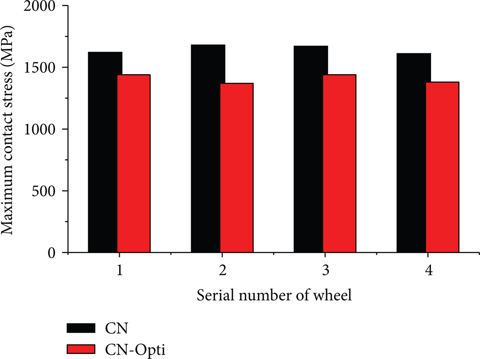
Contact stress comparison of CN and CN-OPTI profiles.

7.4.4. Wheel/Rail Dynamics Analysis

Certain wheel/rail dynamic properties such wheel/rail lateral force, front and back bogie acceleration, and derailment coefficient of both the CN-Opti and CN profiles are analyzed, as shown in Figures 8, 9, and 10. Using the CN-Opti profile, the RMS of lateral force of the left wheel is reduced to 8.51 KN from the original 10.27 KN, a 17.1% decrease; lateral force of the right wheel is reduced to 8.07 KN from the original 9.45 KN, a 14.6% decrease. Except for a few cases where maximum acceleration of front and back bogies is greater than the original values, generally the RMS of the front and back bogie acceleration are reduced by 8.6% and 9.8%, respectively. The derailment coefficient also decreases over the entire line, where the RMS value of derailment coefficient of the left wheel is reduced from the original 0.095 to 0.089, a 6.3% decrease; for the right wheel, there is a reduction from the original 0.093 to 0.880, a 5.3% decrease.

Figure 8:

Comparison of wheel/rail lateral force of CN and CN-Opti profiles.

Figure 9:

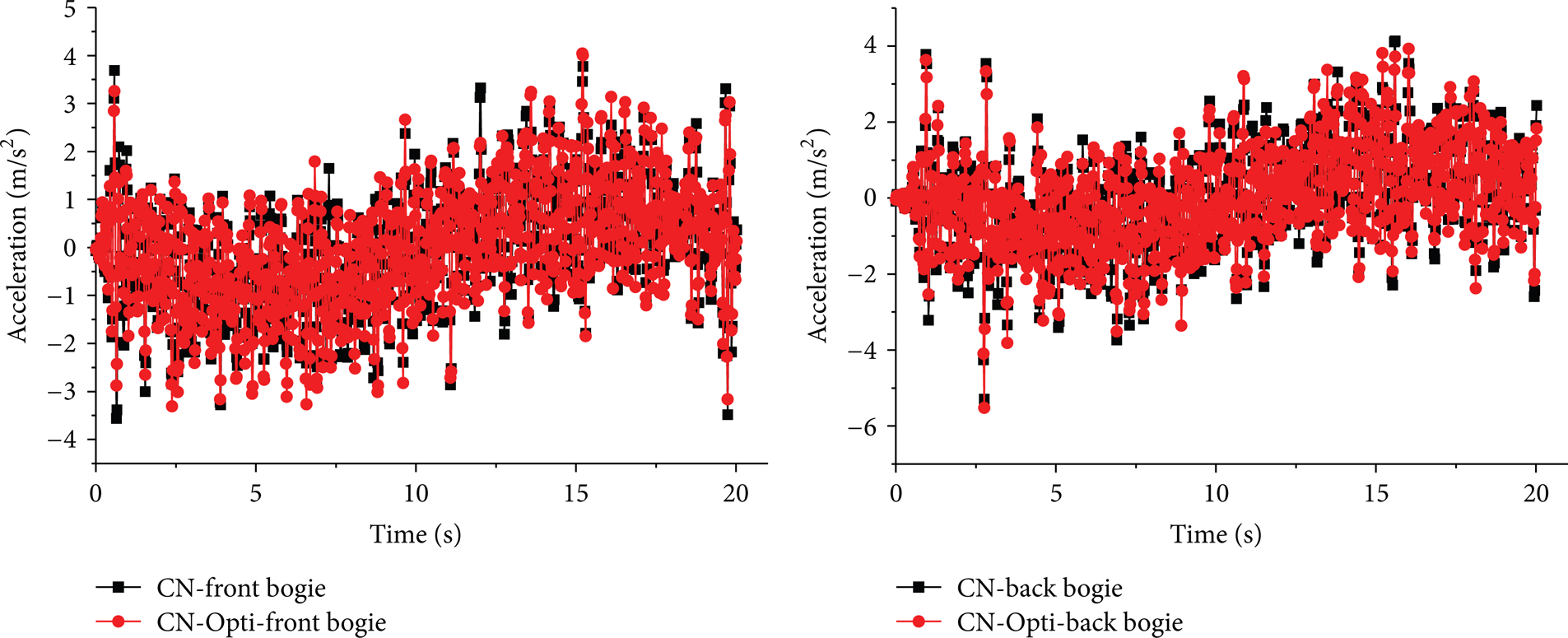
Comparison of bogie acceleration of CN and CN-Opti profiles.

Figure 10:

Comparison of derailment coefficient of CN and CN-Opti profiles.

Between Figures 8 and 10 it becomes clear that rail wear is reduced when CN-Opti is used. Because the CN_Opti tread primarily contacts the rail top profile and the arc radius of the rail is 300 m, the wheel-rail contact area is larger. The smaller wheel and rail contact stress and creep force help to slow down the wheel-rail wear. Compared to the CN-Opti/CHN60 pair, the wheel flange contact with the rail side is greater for the CN/CHN60 pair in a case with large lateral displacement in the curve negotiation. A mutation point emerged on the equivalent conicity curve, and the increasing rolling radius difference as y is bigger than 8.2 mm for the CN profile significantly affects the lateral vibration and thus the safety of the vehicle. The optimized CN-Opti profile helps prevent jump contact and flange contact with the rail side, which contributes favorably to lateral force, decreases derailment coefficient, and improves vehicle lateral vibration.

7.4.5. Curving Performance

The maximum derailment coefficient and load reduction rate improved considerably; in general, effectively cutting the maximum derailment coefficient and wheel load reduces ratio by up to 19.8% and 11.4%, respectively. As vehicles pass through the track, described in Section 7.4.1, their speed is within 200–300 km/h. Figure 11 shows comparison results of maximum derailment coefficient and load reduction in the curve negotiation.

Figure 11:

Comparison of max derailment coefficient and load reduction of CN and CN-Opti profiles.

8. Conclusion

(1) The CN wheel profile of CRH3 EMU was evenly divided into 14, 19, and 24 arcs with 15, 20, and 25 discrete points selected as data points. NURBS theory was then used to build a CN profile, which had correlation coefficients of 0.83, 0.93, and 0.95, respectively, with the original CN standard curve. Comparative analysis indicated that dividing the profile into 19 arcs, that is, 20 data points, for curve regeneration formed the most accurate description of the wheel profile.

(2) Vertical coordinates of the 20 data points on the wheel profile were selected as design variables. Objective function was established to identify the minimum mean wear work and the minimum wheel/rail lateral force of the first wheelset. Constraint function was also established with statistics of worn wheel profiles, convexity, and continuity of the profile as geometric constraint conditions. Both were multiobjectively optimized to complete wheel profiles.

(3) The PSO method was used to find a solution for the optimization model. Results showed that, for the optimized CN-Opti profile, the contact distribution mainly concentrated on the wheel tread and rail top and less on the point of flange contact with the rail side. Vehicle critical speed for CN-Opti and CN wheel profiles was 575 km/h and 530 km/h, respectively. The mean wear work of the first wheelset of the CN-Opti profile was reduced by 18.8% compared to the CN profile. The maximum contact stress of all four wheels in the first and second wheelsets decreased by 11.11%–18.45%. The RMS values of lateral forces of both the left and right wheels were, respectively, reduced by 17.1% and 14.6%. The maximum derailment coefficient and load reduction rate were reduced up to 19.8% and 11.4%, respectively. Analysis has indicated that overall the optimized CN-Opti profile shows better, comprehensive, dynamic characteristics than the CN profile.

Conflict of Interests

The authors declare that there is no conflict of interests regarding the publication of this paper.