Survivability-Aware Topology Evolution Model with Link and Node Deletion in Wireless Sensor Networks

Abstract

The paper proposes the algorithm of survival topology evolution model. The model applies the survival analysis to the research on the topology of networks. On one hand, it takes the survivability of every node into account. Since the state of a node is affected by the node itself, the environment and so on, it's necessary to study the survivability of nodes. In addition, the survival analysis on the nodes can indicate whether the nodes work well in real time. On the other hand, it also takes the deletion of links and nodes determined by the survivability of the nodes into account. Then it reaches the conclusion by mean field method. The result shows that the degree distributions of WSNs are approximately power law as B-A model and that the survivability of the nodes is proportional to the degree distribution of the network consisting of the previous nodes. These are further confirmed by simulation example.

1. Introduction

Wireless sensor network (WSN) appears with the rapid development of microelectromechanical systems (MEMS), system on a chip (SoC), wireless communication, and low-power embedded technology, which brings a revolution of information perception. WSN is a multiple hops self-organizing network which is made of a large number of low-cost microsensor nodes deployed in the monitoring area by wireless communication. As the scale of WSN becomes larger and larger, the problem of coefficient, error, and attack tolerance arouses people's concern. Hence, it is necessary to find the solution.

In recent years, people pay more and more attention to the structure and dynamics of large complex networks [1]. Many new topology algorithms for wireless sensor networks have been presented due to the influence the topology has on the lifetime and communication efficiency of a network. In [2], a complex networks-based energy-efficient evolution model for wireless sensor networks is proposed. In [3], the authors presented a local world evolving model for energy-constrained wireless sensor networks. In [4], an energy-aware topology evolution model with link and node deletion in wireless sensor networks is presented. In [5], an evolving model of network with aging sites was proposed according to the effect of aging on network structure presented in [6, 7]. The model applies the algorithm proposed in [8–11] such as the mean field theory to the algorithm in [5]. In [12], the authors proposed a weighted local world evolving network model with aging nodes to make the previous model portray some complex networks more appropriately.

The models above are all involved in the energy of a node. And the topology of a WSN is closely related to it. However, what impacts the lifetime of a node is not only the energy. As a result, the paper takes the notion of survivability into account. Survival analysis refers to making an analysis and inference on the survival time of creatures and people according to the data from tests or investigations. With the continuous improvement of the theories and methods of survival analysis, survival analysis comes to be applied to some other fields such as the assessment of the lifetime of products.

Survival analysis has become another hot topic in recent years. Although it is proposed to solve some biology problems, people are focusing on its application to computer science [13]. For example, the articles [14–19] are trying to give a three-layer survivability analysis on the reliability of the WSN. As we all know, the WSN consists of plenty of inexpensive sensor nodes, which are not repairable and worthy of repairing. Therefore, the lifetime of the sensor nodes is limited. And the WSN is generally deployed in the severe environment, which will shorten the lifetime of the nodes. And then it is necessary to consider the survivability of the nodes when studying the topology of the WSN. So this paper applies the survivability of every node to the energy-aware topology evolution model with link and node deletion and then explores the topology of WSN.

The remainder of the paper is made of three sections. In Section 2, an algorithm of survival topology evolution model, which is based on [4], is proposed. In Section 3, the numerical experiments to present the features of the networks generated by the proposed algorithm are given. Finally, some concluding remarks are given in Section 4.

2. Model

The particular features of WSNs evolving networks can be captured in the present model. The model evolves from an initial WSN consisting of $n_{\mathrm{0}}$ nodes and $e_{\mathrm{0}}$ edges.

2.1. Preferential Attachment

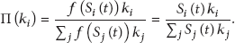
The survivability of the nodes in a WSN has an impact on the lifetime of the network, which will influence the topology of the network at the same time. As we all know, the survivability of a node is not only related to the energy of the node, but also involved in other factors such as the disturbance in the environment. The section is doing some researches on how the survivability of the nodes impacts the topology of a WSN. In other words, the model takes the energy of the node, the disturbance in the environment, and so on into account. Then, the iterative algorithm during the evolving process is outlined as follows.

At each time step, a new node is added to the system. And $m\hspace{0.17em}\hspace{0.17em}(\mathrm{0}<m<n_{\mathrm{0}})$ new links from the new node are connected to existing nodes [1]. We assume that the probability ${\Pi }_i$ of a new node will be connected to node i depends on the connectivity $k_i$ and the survivability of the node i. In this paper, we define a function $f(S(t))$ to represent the relationship between the survivability of a node and its ability to be linked. The more survivability of a node is, the more ability it will have of being connected to the new coming nodes. Therefore, $f(S(t))$ must be an increasing function and the form may be $S(t)$ , $[S(t){]}^{\mathrm{2}}$ , $\sqrt{S(t)}$ , $\ln [S(t)]$ , and so on. In this paper, we just set $f(S_i(t))=S_i(t)$ . And the form of ${\Pi }_i$ is

$$\begin{array}{cc}& \Pi \left(k_i\right)=\frac{f\left(S_i\left(t\right)\right)k_i}{{\sum }_j‍f\left(S_j\left(t\right)\right)k_j}=\frac{S_i\left(t\right)k_i}{{\sum }_j‍S_j\left(t\right)k_j}.\end{array}$$

(1)

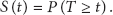
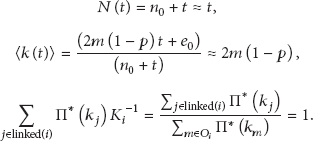
From [13], the survivability $S(t)$ of a node is defined as the probability that the life T of the node exceeds the time $t\hspace{0.17em}\hspace{0.17em}(t>\mathrm{0})$ :

$$\begin{array}{cc}& S\left(t\right)=P\left(T\ge t\right).\end{array}$$

(2)

2.2. Links Deletion

At each time, with probability $p\hspace{0.17em}\hspace{0.17em}(\mathrm{0}\le p<\mathrm{1})$ , $m*p$ old links are removed. So the parameter p denotes the deletion rate, which is defined as the rate of links removed divided by the rate of links addition; see [4]. We assume the value of the parameter p is related to the survivability $S(t)$ of the node. In this paper, we assume the survivability of a node is related to the definition of the deletion rate p as follows.

We set a survival function threshold $n\hspace{0.17em}\hspace{0.17em}(\mathrm{0}<n<\mathrm{1})$ . If the survivability of a node satisfies

$$\begin{array}{cc}& S\left(t\right)=P\left(T\ge t\right)<n\end{array}$$

(3)

then the node will be removed. So the deletion rate of the node can be expressed as the probability that the survivability of the node is lower than the threshold n:

$$\begin{array}{cc}& p=P\left\{S\left(t\right)<n\right\}=P\left\{P\left(T\ge t\right)<n\right\}.\end{array}$$

(4)

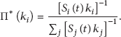
We first select a node i as an end of a deleted link with the antipreferential probability as

$$\begin{array}{cc}& {\Pi }^{*}\left(k_i\right)=\frac{{\left[S_i\left(t\right)k_i\right]}^{-\mathrm{1}}}{{\sum }_j‍{\left[S_j\left(t\right)k_j\right]}^{-\mathrm{1}}}.\end{array}$$

(5)

The less energy the node has, the more probability it will have for being deleted.

Then node j is then chosen from the linked neighborhood of node i (denoted by $O_i$ ) with probability ${K_i}^{-\mathrm{1}}{\Pi }^{*}(k_j)$ , where $K_i={\sum }_{j\in O_i}‍{\Pi }^{*}(k_j)$ . Then the link connecting nodes i and j is removed; this process is repeated $m*p$ times. Once an isolated node appears, it should be removed from the network to maintain the connectivity of networks.

2.3. Degree Distribution

In complex networks, the degree distribution $P(k)$ , which indicates the probability that a randomly selected node has k connections, is a very important and useful factor to observe the features of networks and has been suggested to be used as the first criterion to classify real-world networks. In this paper, the mean field theory is adopted to give a qualitative analysis of $P(k)$ for our survivability-aware evolving model with link and node deletions.

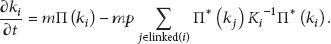
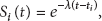
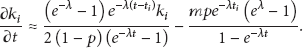
By the mean field theory, let $k_i(t)$ be the degree of the ith node at time t, and then, in the limit of large t, the increasing rate of $k_i(t)$ satisfies the following dynamical equation:

$$\begin{array}{cc}& \frac{\partial k_i}{\partial t}=m\Pi \left(k_i\right)-mp{{\displaystyle \sum }}_{j\in \text{linked}\left(i\right)}‍{\Pi }^{*}\left(k_j\right){K_i}^{-\mathrm{1}}{\Pi }^{*}\left(k_i\right).\end{array}$$

(6)

The first term in (6) accounts for the increasing number of links of the ith node by the preferential attachment due to the newly added node. The second item in (6) means the losing of links by antipreferential attachment during the evolving process.

From the mean field sense, we have

$$\begin{array}{cc}& {{\displaystyle \sum }}_j‍S_j\left(t\right)k_j=N\left(t\right)*\stackrel{-}{S}\left(t\right)*〈k\left(t\right)〉,\end{array}$$

(7)

where $\stackrel{-}{S}(t)$ is the expected value of the node survivability in the whole network; $N(t)$ is the number of nodes at time t;   $〈k(t)〉$ is the average degree of the network at time t. For large t,

$$\begin{array}{cc}& N\left(t\right)=n_{\mathrm{0}}+t\approx t,\\ 〈k\left(t\right)〉=\frac{\left(\mathrm{2}m\left(\mathrm{1}-p\right)t+e_{\mathrm{0}}\right)}{\left(n_{\mathrm{0}}+t\right)}\approx \mathrm{2}m(\mathrm{1}-p),\\ {{\displaystyle \sum }}_{j\in \text{linked}\left(i\right)}‍{\Pi }^{*}\left(k_j\right){K_i}^{-\mathrm{1}}=\frac{{\sum }_{j\in \text{linked}\left(i\right)}‍{\Pi }^{*}\left(k_j\right)}{{\sum }_{m\in O_i}‍{\Pi }^{*}\left(k_m\right)}=\mathrm{1}.\end{array}$$

(8)

In this paper, we assume that the survivability of nodes is exponential distribution as the following:

$$\begin{array}{cc}& S_i\left(t\right)=e^{-\lambda \left(t-t_i\right)},\end{array}$$

(9)

where $t_i$ indicates the time a new node is added to the network and $\lambda \hspace{0.17em}\hspace{0.17em}(\lambda >\mathrm{0})$ is a parameter of the exponential distribution. Then the expected node survivability in the whole network is

$$\begin{array}{l}\stackrel{-}{S}\left(t\right)=\frac{{\sum }_i‍S_i\left(t\right)}{N\left(t\right)}\\ \approx \frac{e^{-\lambda (t-\mathrm{1})}+e^{-\lambda (t-\mathrm{2})}+\cdots +e^{-\lambda (t-t)}}{t}\\ =\frac{e^{-\lambda t}-\mathrm{1}}{t\left(e^{-\lambda }-\mathrm{1}\right)}.\end{array}$$

(10)

Finally, we can get the simplified form of the dynamical equation:

$$\begin{array}{cc}& \frac{\partial k_i}{\partial t}\approx \frac{\left(e^{-\lambda }-\mathrm{1}\right)e^{-\lambda (t-t_i)}{k}_i}{\mathrm{2}(\mathrm{1}-p)(e^{-\lambda t}-\mathrm{1})}-\frac{mp{e}^{-\lambda t_i}(e^{\lambda }-\mathrm{1})}{\mathrm{1}-e^{-\lambda t}}.\end{array}$$

(11)

2.4. Calculation

2.4.1. Case A $(p\hspace{0.17em}\mathbf{=}\hspace{0.17em}0)$

In this case, there are only link and node additions without link and node deletions in the evolving process. It is usually fit for topology discovery state of WSNs in which all nodes have enough survivability in the ideal environment. So $k_i(t)$ satisfies

$$\begin{array}{cc}& \frac{\partial k_i}{\partial t}\approx \frac{\left(e^{-\lambda }-\mathrm{1}\right)e^{-\lambda \left(t-t_i\right)}{k}_i}{\mathrm{2}\left(e^{-\lambda t}-\mathrm{1}\right)}.\end{array}$$

(12)

With the initial condition $k_i(t)=m$ , then we can get

$$\begin{array}{cc}& k_i\left(t\right)=m{\left(\frac{\mathrm{1}-e^{-\lambda t_i}}{\mathrm{1}-e^{-\lambda t}}\right)}^{-(e^{-\lambda }-\mathrm{1})e^{\lambda t_i}/\mathrm{2}\lambda }.\end{array}$$

(13)

The probability that a node has a connectivity which satisfies $k_i(t_i)<k$ is

$$\begin{array}{l}P\left(k_i<k\right)=P\left(m{\left(\frac{\mathrm{1}-e^{-\lambda t_i}}{\mathrm{1}-e^{-\lambda t}}\right)}^{-(e^{-\lambda }-\mathrm{1})e^{\lambda t_i}/\mathrm{2}\lambda }<m\right)\\ \approx P\left(t_i>\frac{\mathrm{1}}{\lambda }\ln \left(A+e^{\lambda t}-A\frac{k}{m}\right)\right),\end{array}$$

(14)

where $A=\mathrm{2}\lambda (\mathrm{1}-e^{-\lambda t})/(e^{-\lambda }-\mathrm{1})e^{-\lambda t}$ .

Assuming that we add the node to the network at equal time intervals in evolving process for WSNs, the probability density at the time $t_i$ is $P(t_i)=\mathrm{1}/(n_{\mathrm{0}}+t)$ . Therefore, we get

$$\begin{array}{cc}& P\left(k_i<k\right)=\frac{\mathrm{1}}{\lambda \left(n_{\mathrm{0}}+t\right)}\ln \left(A+e^{\lambda t}-A\frac{k}{m}\right).\end{array}$$

(15)

The probability density function of the degree of a node is

$$\begin{array}{cc}& \frac{\partial P(k_i<k)}{\partial k}=\frac{\mathrm{1}}{\lambda \left(n_{\mathrm{0}}+t\right)}\frac{-A\left(\mathrm{1}/m\right)}{A+e^{\lambda t}-A\left(k/m\right)}.\end{array}$$

(16)

2.4.2. Case B $\mathbf{(}p\mathbf{\ne }0\mathbf{)}$

In this case, links and nodes in the evolving network model are not monotonously growing. Instead, links and nodes can be added in some occasions and removed in other cases.

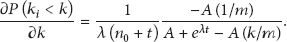
At first, we assume the probability density of the threshold n is 1. Then we can obtain the expression of p from (4) and (9)

$$\begin{array}{l}p=P\{S\left(t\right)<n\}\\ =P\{n>P(T\ge t)\}\\ =\mathrm{1}-P\{n-P(T\ge t)\}=\mathrm{1}-e^{-\lambda t}.\end{array}$$

(17)

Here, we assume $t\gg t_i$ . Then we can get (18) from (11)

$$\begin{array}{cc}& \frac{\partial k_i}{\partial t}\approx \frac{(e^{-\lambda }-\mathrm{1})e^{-\lambda (t-t_i)}{k}_i}{\mathrm{2}{e}^{-\lambda t}(e^{-\lambda t}-\mathrm{1})}-m{e}^{-\lambda t_i}(e^{\lambda }-\mathrm{1}).\end{array}$$

(18)

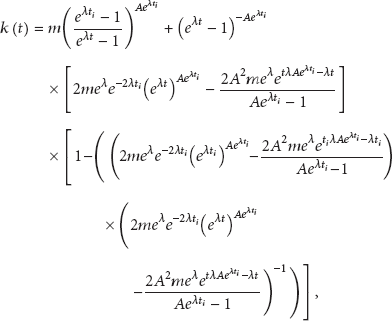
By solving the differential equation (18), we can get the form of the solution to the differential equation as follows:

$$\begin{array}{l}k\left(t\right)=C{e}^{-\int ‍P\left(t\right)dt}\\ \hspace{1em}+e^{-\int ‍P\left(t\right)dt}*{\displaystyle \int }‍Q\left(t\right)*e^{\int ‍P\left(t\right)dt}dt,\end{array}$$

(19)

where

$$\begin{array}{cc}& P\left(t\right)=-\frac{\left(e^{-\lambda }-\mathrm{1}\right)e^{-\lambda \left(t-t_i\right)}}{\mathrm{2}{e}^{-\lambda t}\left(e^{-\lambda t}-\mathrm{1}\right)},\\ Q\left(t\right)=-m{e}^{-\lambda t_i}(e^{\lambda }-\mathrm{1}).\end{array}$$

(20)

With the same initial condition as Case  A, $k_i(t_i)=m$ , the solution will be (21) after simplification. Consider

$$\begin{array}{l}k\left(t\right)=m{\left(\frac{e^{\lambda t_i}-\mathrm{1}}{e^{\lambda t}-\mathrm{1}}\right)}^{A{e}^{\lambda t_i}}+{\left(e^{\lambda t}-\mathrm{1}\right)}^{-A{e}^{\lambda t_i}}\\ \times \left[\mathrm{2}m{e}^{\lambda }{e}^{-\mathrm{2}\lambda t_i}{\left(e^{\lambda t}\right)}^{A{e}^{\lambda t_i}}-\frac{\mathrm{2}{A}^{\mathrm{2}}m{e}^{\lambda }{e}^{t\lambda A{e}^{\lambda t_i}-\lambda t}}{A{e}^{\lambda t_i}-\mathrm{1}}\right]\\ \times [1-(\phantom{{\hspace{1em}\hspace{1em}\hspace{1em}\hspace{1em}\hspace{1em}-\frac{\mathrm{2}{A}^{\mathrm{2}}m{e}^{\lambda }{e}^{t\lambda A{e}^{\lambda t_i}-\lambda t}}{A{e}^{\lambda t_i}-\mathrm{1}})}^{-1}}\left(\mathrm{2}m{e}^{\lambda }{e}^{-\mathrm{2}\lambda t_i}{\left(e^{\lambda t_i}\right)}^{A{e}^{\lambda t_i}}-\frac{\mathrm{2}{A}^{\mathrm{2}}m{e}^{\lambda }{e}^{t_i\lambda A{e}^{\lambda t_i}-\lambda t_i}}{A{e}^{\lambda t_i}-\mathrm{1}}\right)\\ \times (\phantom{-\frac{\mathrm{2}{A}^{\mathrm{2}}m{e}^{\lambda }{e}^{t\lambda A{e}^{\lambda t_i}-\lambda t}}{A{e}^{\lambda t_i}-\mathrm{1}}}\mathrm{2}m{e}^{\lambda }{e}^{-\mathrm{2}\lambda t_i}{\left(e^{\lambda t}\right)}^{A{e}^{\lambda t_i}}\\ \hspace{0.5em}\hspace{0.17em}{\hspace{1em}\hspace{1em}\hspace{1em}\hspace{1em}\hspace{1em}-\frac{\mathrm{2}{A}^{\mathrm{2}}m{e}^{\lambda }{e}^{t\lambda A{e}^{\lambda t_i}-\lambda t}}{A{e}^{\lambda t_i}-\mathrm{1}})}^{-1})],\end{array}$$

(21)

where $A=(e^{-\lambda }-\mathrm{1})/\mathrm{2}\lambda$ .

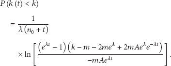
Then the probability that a node has a connectivity which satisfies $k_i(t_i)<k$ is

$$\begin{array}{l}P(k\left(t\right)<k)\\ \hspace{1em}\approx P(m{\left(\frac{e^{\lambda t_i}-\mathrm{1}}{e^{\lambda t}-\mathrm{1}}\right)}^{A{e}^{\lambda t_i}}+{\left(e^{\lambda t}-\mathrm{1}\right)}^{-A{e}^{\lambda t_i}}\\ \times [\mathrm{2}m{e}^{\lambda }{e}^{-\mathrm{2}\lambda t_i}{\left(e^{\lambda t}\right)}^{A{e}^{\lambda t_i}}\phantom{m{\left(\frac{e^{\lambda t_i}-\mathrm{1}}{e^{\lambda t}-\mathrm{1}}\right)}^{A{e}^{\lambda t_i}}+{\left(e^{\lambda t}-\mathrm{1}\right)}^{-A{e}^{\lambda t_i}}}\\ \hspace{1em}\hspace{1em}\hspace{1em}\hspace{1em}\phantom{m{\left(\frac{e^{\lambda t_i}-\mathrm{1}}{e^{\lambda t}-\mathrm{1}}\right)}^{A{e}^{\lambda t_i}}+{\left(e^{\lambda t}-\mathrm{1}\right)}^{-A{e}^{\lambda t_i}}}-\frac{\mathrm{2}{A}^{\mathrm{2}}m{e}^{\lambda }{e}^{t\lambda A{e}^{\lambda t_i}-\lambda t}}{A{e}^{\lambda t_i}-\mathrm{1}}]<k).\end{array}$$

(22)

Assuming that we add the node to the network at equal time intervals in evolving process for WSNs, the probability density at the time $t_i$ is $P(t_i)=\mathrm{1}/(n_{\mathrm{0}}+t)$ . Therefore, we get

$$\begin{array}{l}P\left(k\left(t\right)<k\right)\\ \hspace{1em}=\frac{\mathrm{1}}{\lambda \left(n_{\mathrm{0}}+t\right)}\\ \hspace{1em}\hspace{1em}\times \ln \left[\frac{\left(e^{\lambda t}-\mathrm{1}\right)\left(k-m-\mathrm{2}m{e}^{\lambda }+\mathrm{2}mA{e}^{\lambda }{e}^{-\lambda t}\right)}{-mA{e}^{\lambda t}}\right].\end{array}$$

(23)

The probability density function of the degree of a node is

$$\begin{array}{cc}& P\left(k\right)=\frac{\mathrm{1}}{\lambda \left(n_{\mathrm{0}}+t\right)}*\frac{\mathrm{1}}{k-m-\mathrm{2}m{e}^{\lambda }+\mathrm{2}mA{e}^{\lambda }{e}^{-\lambda t}}.\end{array}$$

(24)

3. Simulation

In this section, we compute numerical results in the evolution of a network and compare them with simulation examples.

3.1. Case A $\mathbf{(}p\hspace{0.17em}\mathbf{=}\hspace{0.17em}0\mathbf{)}$

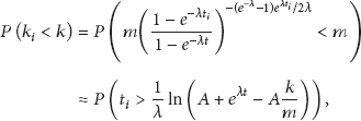
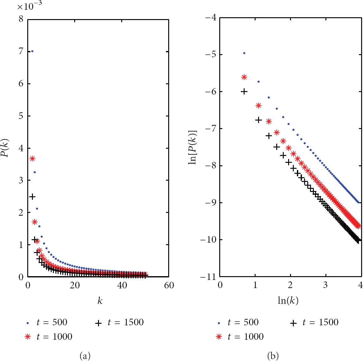
The degree distribution $P(k)$ is provided for different time t with fixed $\lambda =\mathrm{0.3}$ , $n_{\mathrm{0}}=\mathrm{50}$ , $m=\mathrm{2}$ in Figure 1. According to (15), k must satisfy the following condition to guarantee nonnegativity of $P(k)$ , which is consistent with the other expressions:

$$\begin{array}{cc}& k>m+\frac{m}{A}{e}^{\lambda t}.\end{array}$$

(25)

It indicates that the degree distributions $P(k)$ are approximately power law as B-A model. Figure 1(a) shows that the network makes lower connectivity as t increases, because the scale of the network becomes larger with the increment of t. Although the probability of a node to be connected becomes bigger as time goes on, the number of nodes in the network becomes larger at the same time. Of course, the survivability of nodes becomes smaller as time goes on, which is also the reason of lower connectivity as t increases. Figure 1(b) shows that the degree distribution $P(k)$ follows an approximate exponential decay with the increase of k and the rate of decay will be much faster with the growth of time.

Figure 1

The degree distribution $P(k)$ in comparison with different $t\hspace{0.17em}\hspace{0.17em}(\lambda =\mathrm{0.3}$ ,   $n_{\mathrm{0}}=\mathrm{50}$ ,   $m=\mathrm{2})$ .

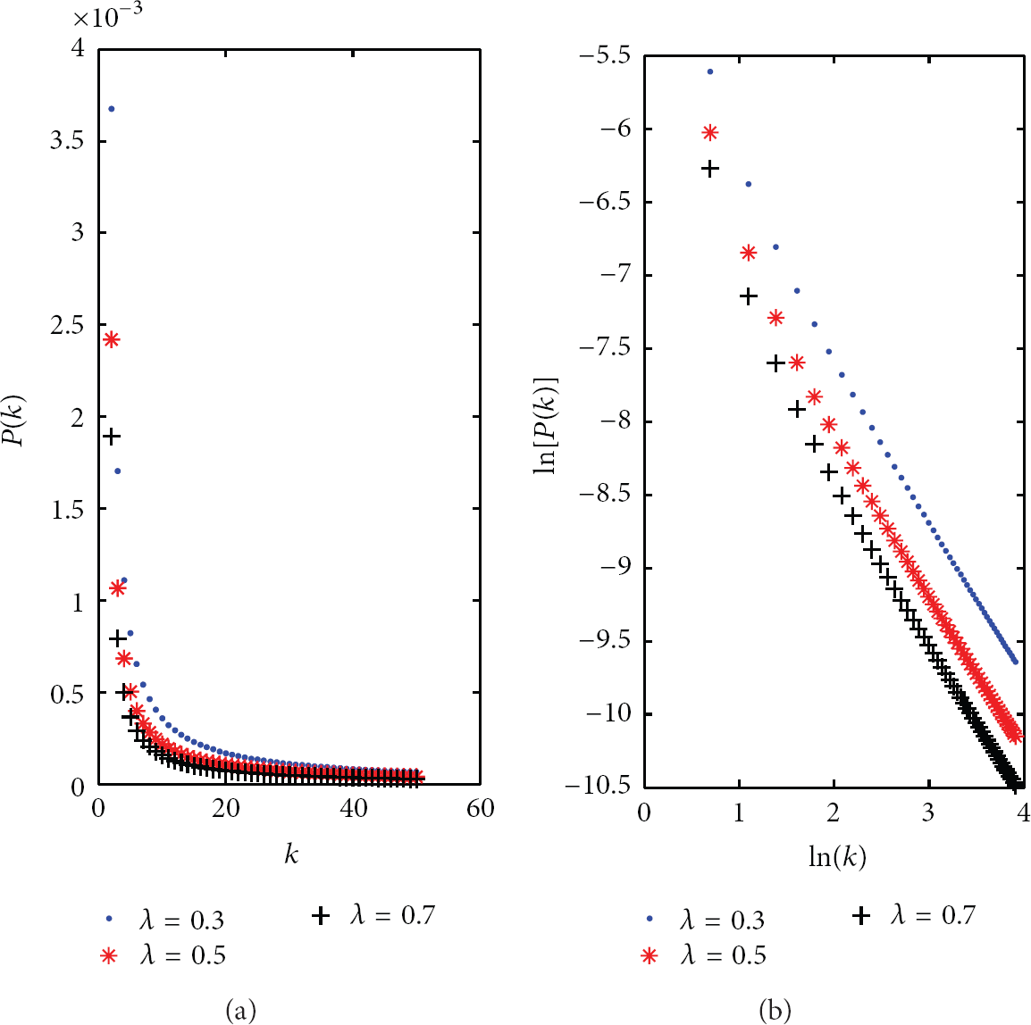
The degree distribution $P(k)$ is provided for different time λ with fixed $t=\mathrm{1000}$ , $n_{\mathrm{0}}=\mathrm{50}$ , $m=\mathrm{2}\lambda =\mathrm{0.3}$ , $n_{\mathrm{0}}=\mathrm{50}$ , $m=\mathrm{2}$ in Figure 2. It indicates that the network makes higher connectivity as λ decreases. Figure 2(a) shows that when the survivability of the nodes in the network becomes lower with the increment of λ, the probability of the nodes to be connected will be higher, which is the same with the definition of (1). Figure 2(b) shows that the degree distribution $P(k)$ follows an approximate exponential decay with the increment of k and the rate of decay will be much faster with the growth of λ.

Figure 2

The degree distribution $P(k)$ in comparison with different $\lambda \hspace{0.17em}\hspace{0.17em}(t=\mathrm{1000}$ ,   $n_{\mathrm{0}}=\mathrm{50}$  ,  $m=\mathrm{2})$ .

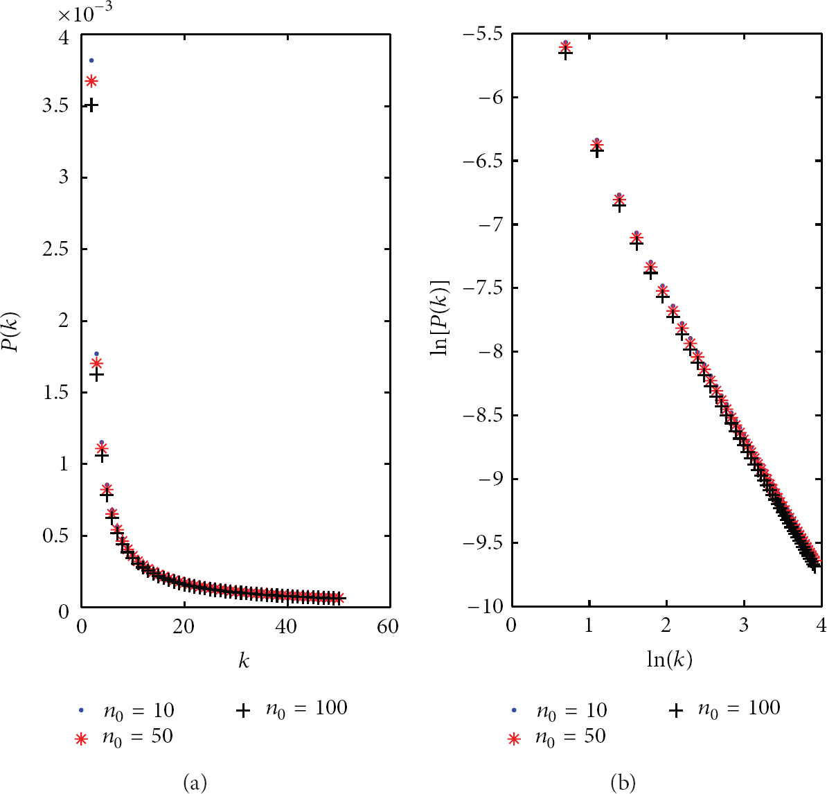
The degree distribution $P(k)$ is provided for different time $n_{\mathrm{0}}$ with fixed $t=\mathrm{1000}$ , $\lambda =\mathrm{0.3}$ , $m=\mathrm{2}$ in Figure 3. Figure 3(a) shows that the network yields higher connectivity as $n_{\mathrm{0}}$ decreases. It is concluded that the degree distribution $P(k)$ follows an approximate exponential decay with the increase of k and the rate of decay will be much faster with the growth of $n_{\mathrm{0}}$ .

Figure 3

The degree distribution $P(k)$ in comparison with different $n_{\mathrm{0}}\hspace{0.17em}\hspace{0.17em}(t=\mathrm{1000},\hspace{0.17em}\hspace{0.17em}\lambda =\mathrm{0.3},\hspace{0.17em}\hspace{0.17em}m=\mathrm{2})$ .

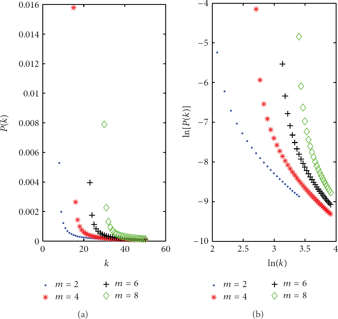
The degree distribution $P(k)$ is provided for different time m with fixed $t=\mathrm{1000}$ , $\lambda =\mathrm{0.3}$ , $n_{\mathrm{0}}=\mathrm{50}$ in Figure 4. Figure 4(a) shows that with the increase of the value of m, the beginning of the curve gradually moves to right, which is determined from (25). It is also very easy to understand that the network makes higher connectivity as m increases. Hence, Figure 4(b) shows that the degree distribution $P(k)$ follows an approximate exponential decay with the increase of $P(k)$ and the greater the m is, the faster the rate of the decay will be from Figure 4.

Figure 4

The degree distribution $P(k)$ in comparison with different $m\hspace{0.17em}\hspace{0.17em}(t=\mathrm{1000},\hspace{0.17em}\hspace{0.17em}\lambda =\mathrm{0.3},\hspace{0.17em}\hspace{0.17em}{n}_{\mathrm{0}}=\mathrm{50})$ .

3.2. Case B $\mathbf{(}p\mathbf{\ne }0\mathbf{)}$

The degree distribution $P(k)$ is provided for different time t with fixed $\lambda =\mathrm{0.3}$ , $n_{\mathrm{0}}=\mathrm{50}$ , $m=\mathrm{2}$ in Figure 5. According to (23), k must satisfy the following condition to ensure nonnegativity of $P(k)$

$$\begin{array}{cc}& k>m+\mathrm{2}m{e}^{\lambda }-\mathrm{2}mA{e}^{\lambda }{e}^{-\lambda t}.\end{array}$$

(26)

It can be found that the degree distributions $P(k)$ are approximately power law as B-A model because the survivability of the nodes will become lower as time goes on. Figure 5(a) shows that the network makes higher connectivity as t increases, because the scale of the network becomes larger with the increase of t, which is the same with Case A. In addition, the value of $P(k)$ is higher when k is comparatively smaller due to the limitation to the lifetimes of nodes. Figure 5(b) shows that the degree distribution $P(k)$ follows an approximate exponential decay with the increase of $P(k)$ .

Figure 5

The degree distribution $P(k)$ in comparison with different $t\hspace{0.17em}\hspace{0.17em}(\lambda =\mathrm{0.3},\hspace{0.17em}\hspace{0.17em}{n}_{\mathrm{0}}=\mathrm{50},\hspace{0.17em}\hspace{0.17em}m=\mathrm{2})$ .

The degree distribution $P(k)$ is provided for different time λ with fixed $t=\mathrm{1000}$ , $n_{\mathrm{0}}=\mathrm{50}$ , $m=\mathrm{2}$ in Figure 6. In Case B, the nodes and links are deleted according to the survivability of the nodes, so when the value of λ becomes bigger, that is to say, the survivability of the nodes becomes lower, the nodes and its links will be easier to be deleted. Consequently, the values of $P(k)$ are bigger at the beginning of the curves with the smaller λ. According to (26), the curve with bigger value of λ begins where the value of k is bigger. Due to the survivability, the values of $P(k)$ with bigger λ will become smaller with the increment of k. So some intersections will be shown in Figure 6(a). Figure 6(b) shows that the degree distribution $P(k)$ follows an approximate exponential decay with the increase of $P(k)$ .

Figure 6

The degree distribution $P(k)$ in comparison with different $\lambda \hspace{0.17em}\hspace{0.17em}(t=\mathrm{1000},{\hspace{0.17em}\hspace{0.17em}n}_{\mathrm{0}}=\mathrm{50},\hspace{0.17em}\hspace{0.17em}m=\mathrm{2})$ .

The degree distribution $P(k)$ is provided for different time $n_{\mathrm{0}}$ with fixed $t=\mathrm{1000}$ , $\lambda =\mathrm{0.3}$ , $m=\mathrm{2}$ in Figure 7. Figure 7(a) shows that there is an inverse relationship between $n_{\mathrm{0}}$ and $P(k)$ , which can also be seen from (24). Figure 7(b) shows that the degree distribution $P(k)$ follows an approximate exponential decay with the increment of k and the rate of decay will be much faster with the growth of $n_{\mathrm{0}}$ .

Figure 7

The degree distribution $P(k)$ in comparison with different $n_{\mathrm{0}}\hspace{0.17em}\hspace{0.17em}(t=\mathrm{1000},\hspace{0.17em}\hspace{0.17em}\lambda =\mathrm{0.3},\hspace{0.17em}\hspace{0.17em}m=\mathrm{2})$ .

The degree distribution $P(k)$ is provided for different time m with fixed $t=\mathrm{1000}$ , $\lambda =\mathrm{0.3}$ , $n_{\mathrm{0}}=\mathrm{50}$ in Figure 8. Figure 8(a) shows that the curves begin at different places, which is the same with Case A. The bigger the m is, the bigger the value of k at the beginning of the curve will be, which can also be seen in (26). Compared with Case A, the distance of the beginning points with different m becomes bigger, which results from the deletion of nodes and links according to the survivability of nodes. Figure 8(b) shows that the degree distribution $P(k)$ follows an approximate exponential decay with the increase of $P(k)$ .

Figure 8

The degree distribution $P(k)$ in comparison with different $m\hspace{0.17em}\hspace{0.17em}(t=\mathrm{1000},\hspace{0.17em}\hspace{0.17em}\lambda =\mathrm{0.3},\hspace{0.17em}\hspace{0.17em}{n}_{\mathrm{0}}=\mathrm{50})$ .

Compared with Case A, the degree distributions of Case B are bigger because the deletion makes the scale of the network in Case B smaller than that in Case A. And all the degree distributions $P(k)$ follow the approximate exponential decay with the increment of k. The rate of the decay depends on the choice of different parameters.

The evolving algorithms for wireless sensor networks discussed in [2–4] are based on the energy of nodes. And this paper introduces the relationship between the survivability of nodes and the energy of nodes. The survivability of nodes is influenced by the battery consumption of the nodes, the disturbance in the environment, and so forth. It is easy to understand that the decrease of the energy of nodes gives rise to the decline of the survivability of the nodes.

It can reach some conclusions from the simulation above. It indicates that the degree distribution follows approximately power law. And the degree distribution increases with the decrease of the survivability. According to the relationship between survivability and energy, the conclusion is consistent with the conclusion in [2–4].

4. Conclusion

The paper proposes the algorithm of survivability topology evolution model. The model applies the survival analysis to the research on the topology of networks and presents the mathematical results. The lifetime of nodes has a great impact on the wireless sensor network made up of these nodes. So we consider the survival analysis of the nodes. Due to the battery consumption of the nodes, the disturbance in the environment, and so forth, the survivability of the nodes will change in real time, which will get rise to the real-time change of the topology of the WSN. Therefore, it is necessary to take the survivability of nodes into account when the topology of the WSN is studied.

According to the model, the simulation studies of the model are presented. From these results, it reaches the conclusion that the degree distributions $P(k)$ are approximately power law as B-A model. When there is no deletion of nodes and links in the network, the lower the survivability of the nodes is, the bigger the values of $P(k)$ will be. When there is a deletion of nodes and links according to the survivability of the nodes, the same consequence can be obtained. Moreover, the values of the degree distributions $P(k)$ in Case B are bigger than those in Case A.