
Abstract
This paper discusses an autonomous space robot for a truss structure assembly using some reinforcement learning. It is difficult for a space robot to complete contact tasks within a real environment, for example, a peg-in-hole task, because of error between the real environment and the controller model. In order to solve problems, we propose an autonomous space robot able to obtain proficient and robust skills by overcoming error to complete a task. The proposed approach develops skills by reinforcement learning that considers plant variation, that is, modeling error. Numerical simulations and experiments show the proposed method is useful in real environments.
1. Introduction
This study discusses an unresolved robotics issue: how to make a robot autonomous. A robot with manipulative skills capable of flexibly achieving tasks, like a human being, is desired. Autonomy is defined as “automation to achieve a task robustly.” Skills can be considered to be solutions to achieve autonomy. Another aspect of a skill is including a solution method. Most human skill proficiency is acquired by experience. Since how to realize autonomy is not clear, skill development must include solution methods for unknown situations. Our problem is how to acquire skills autonomously, that is, how to robustly and automatically complete a task when the solution is unknown.
Reinforcement learning [1] is a promising solution, whereas direct applications of existing methods with reinforcement learning do not robustly complete tasks. Reinforcement learning is a framework in which a robot learns a policy or a control that optimizes an evaluation through trial and error. It is teacherless learning. By means of reinforcement learning, a robot develops an appropriate policy as mapping from state to action when an evaluation is given. The task objective is prescribed, but no specific action is taught. Reinforcement learning often needs many samples. The large number of samples is due to the large number of states and actions. So, online learning in a real environment is usually impractical. Most learning algorithms consist of two processes [2]: (1) online identification by trial and error sampling and (2) finding the optimal policy for the identified model. These two processes are not separated in typical learning algorithms such as Q-learning [3]. Reinforcement learning is said to be adaptive because it uses online identification and on-site optimal control design. Robustness attained using this adaptability is often impractical. It takes a very long time for online identification by means of trial and error.
In our approach, by learning a robust policy rather than by online identification, reinforcement learning is used to achieve a solution to an unknown task.
Using our approach, this study addresses an autonomous space robot for a truss structure assembly. It is difficult for a space robot to achieve a task, for example, peg-in-hole task, by contact with a real environment, because of the error between the real environment and the controller model. In order to solve the problem, a space robot must autonomously obtain proficiency and robust skills to counter the error in the model. Using the proposed approach, reinforcement learning can achieve a policy that is robust in the face of plant variation, that is, the modeling error. Numerical simulations and experiments show that a robust policy is effective in a real environment and the proposed method is used.
2. Need for Autonomy and Approach
2.1. Need for Autonomy
Autonomy is needed wherever robots work. Below, we discuss why and what kind of autonomy is required [4, 5] for space robots.
Space robots are required to complete tasks in the place of extra vehicular activity by an astronaut. Studies of autonomous systems are needed to realize space robots that can achieve missions under human-operator command. There are many applications for the autonomous space robots [6].
We developed ground experiments to simulate a free-flying space robot under orbital microgravity conditions (Figure 1). Using this apparatus, we have studied robot autonomy. Targeting control-based autonomy, we developed an automatic truss structure assembly, and so forth. However, it has been hard to achieve perfect robot automation because of various factors. To make a robot autonomous in the face of the following challenges, we must
solve problems in the actual robot environment;
operate robustly in the face of uncertainties and variations;
overcome the difficulty of comprehensively predicting a wide variety of states;
identify tasks and find unknown solutions to realize robust robot autonomy.
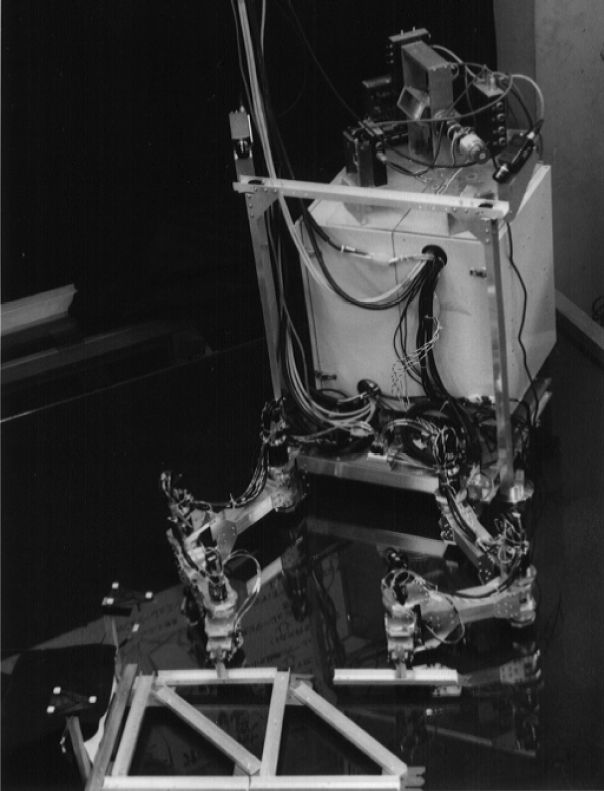
Photograph of space robot model and truss.
2.2. Approach to Autonomy Based on Reinforcement Learning
Human beings achieve tasks regardless of the above complicating factors, but robots cannot. Many discussions have rationalized the difficulties as originating in the nature of human skills. We have not established a means by which we can realize such skills. This study takes the following approach to this problem.
Section 4 approaches factors (a) and (b) in part by way of control-based automation taking account of the robustness of controls. The autonomous level of this approach is low because only small variations are allowable.
Section 5 considers how to surmount factors (a), (b), and (c) by learning. Using a predicted model and transferring the learned results to the actual system [7] is studied. This model is identified online and relearned. This procedure is applied where adaptability or policy modification is needed to thwart variations in the real environment. In some cases, the robot completes the targeted tasks autonomously. Learning is completed within an acceptable calculation time.
Section 6 considers factors (a), (b), (c), and (d). A peg-in-hole task has higher failure rates using the same approach as used in Section 5. Because of small differences between the model and the real environment, failure rates are excessive. The robot thus must gain skills autonomously. Skills similar to those of human beings must be generated autonomously. These skills are developed by reinforcement learning and additional procedures.
Section 7 evaluates approach robustness and control performance of the newly acquired skills. The skills obtained in Section 6 are better than those in Section 5.
3. Experimental System and Tasks
3.1. Outline of Experimental System
Our experimental system (Figures 1 and 2) simulates a free-flying space robot in orbit. Robot model movement is restricted to a two-dimensional plane [5].

Schematic diagram of experimental system.
The robot model consists of a satellite vehicle and dual three degrees of freedom (3-DOF) rigid SCARA manipulators. The satellite vehicle has CCD cameras for stereovision and a position/attitude control system. Each joint has a torque sensor and a servo controller for fine torque control of the output axis. Applied force and torque at the end-effector are calculated using measured joint torque. Air pads are used to support the space robot model on a frictionless planar table and to simulate the space environment. RTLinux is installed on a control computer to control the space robot model in real time. Stereo images from the two CCD cameras are captured by a video board and sent into an image-processing computer with a Windows OS. The image-processing computer measures the position and orientation of target objects in the worksite by triangulation. Visual information is sent to the control computer via Ethernet.
The position and orientation measured by the stereo vision system involve errors caused by quantized images, lighting conditions at the worksite, and so forth. Time-averaged errors are almost constant in each measurement. Evaluated errors in the peg-in-hole experiments are modeled as described below. Hole position errors are modeled as a normal probability distribution, where the mean is m = 0 [mm] and standard deviation is σ = 0.75 [mm]. Hole orientation errors are modeled as a normal probability distribution, where the mean is m = 0 [rad] and standard deviation is σ = 0.5π/180 [rad].
We accomplish a hand-eye calibration to achieve tasks in the following sections. An end-effector, a manipulator hand, grasps a marker with a light-emitting diode (LED). The arm directs the marker to various locations. The robot calculates the marker location by using sensors mounted at the joints of the manipulator arm. The vision system also measures the marker location by using the stereo image by triangulation. Measurements using these joint-angle sensors have more precise resolution and accuracy. Hence, we calibrate the visual measurements based on measurements using the joint angle sensors. We consider the joint angle sensor measurement data to be the true value.
3.2. Tasks
3.2.1. Truss Assembly Task
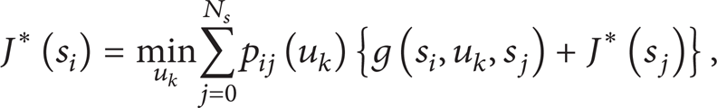
Figure 3 illustrates the truss structure assembly sequence. The robot manipulates a truss component, connects it to a node, and proceeds each assembly step. Later this task is achieved by controls based upon mechanics understanding [5]. The truss design is robot friendly for easy assembling.
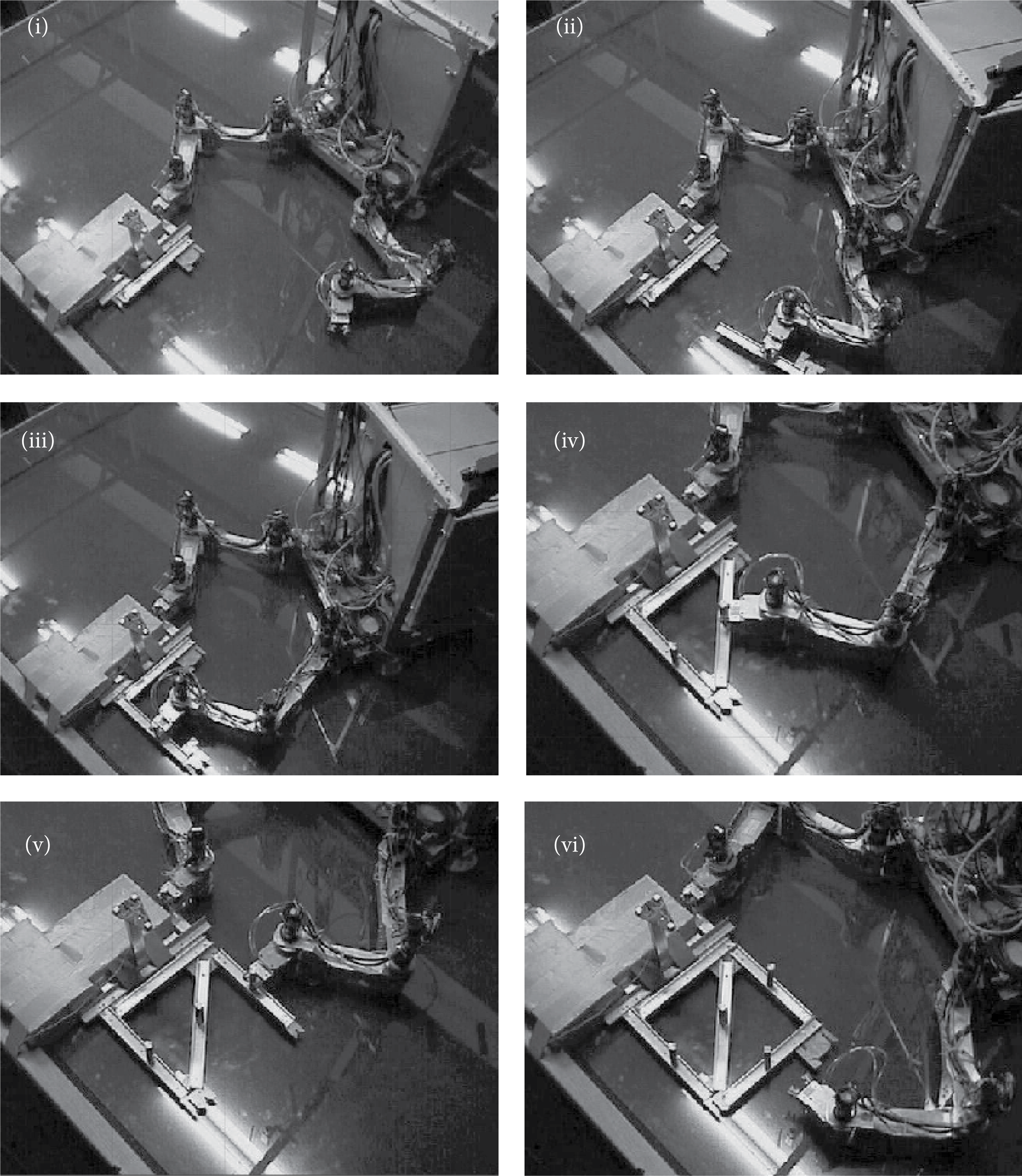
Sequence of truss structure assembly.
3.2.2. Peg-in-Hole Task
The peg-in-hole task is an example that is intrinsic to the nature of assembly. The peg-in-hole task involves interaction within the environment that is easily affected by uncertainties and variations, for example, errors in force applied by the robot, manufacturing accuracy, friction at contact points, and so forth. The peg easily transits to a state in which it can no longer move, for example, wedging or jamming [8]. Such variations cannot be modeled with required accuracy.
To complete a task in a given environment, a proposed method analyzes the human working process and applies the results to a robot [9]. Even if the human skill for a task can be analyzed, the results are not guaranteed to be applicable to a robot. Another method uses parameters in a force control designed by means of a simulation [10] but was not found to be effective in an environment with uncertainty. In yet another method [11], the task achievement ratios evaluated several predesigned paths in an environment with uncertainty. An optimal path is determined among the predesigned paths. There was the possibility a feasible solution did not exist among predesigned paths.
In the peg-in-hole experiment (Figure 4), the position and orientation of the hole are measured using a stereo camera. The robot manipulator inserts a square peg into a similar sized hole. This experiment is a two-dimensional plane problem (Figure 5). The space robot model coordinate system is defined as Σ0, the end-effector coordinate system as Σ
E
, and the hole coordinate system as Σ
hl
. While the space robot completes its task, the robot grasps the structural site with another manipulator; the relative relation between Σ0 and Σ
hl
is fixed. State variables are defined as [y
x
, y
y
, yθ, f
x
, f
y
, fθ], where (y
x
, y
y
) is the position of Σ
E
in Σ0, yθ is the orientation about

Photograph of peg-in-hole experiment setup.

Definition of peg-in-hole task.
The peg width is 74.0 [mm] and the hole width is 74.25 [mm]. The hole is only 0.25 [mm] wider than the peg. The positioning error is composed of the measurement error and the control error. The robot cannot insert the peg in the hole by position control if the positioning error is beyond ± 0.125 [mm]. Just a single measurement error by stereo vision often moves the peg outside of the acceptable region.
4. Control-Based Automation
4.1. Truss Assembly Task
Automatic truss assembly was studied via control-based automation with mechanics understanding. The robot achieved an automatic truss structure assembly [5] by developing basic techniques and integrating them within the experimental system.
The following sensory feedback control [12] is used for controlling manipulators:
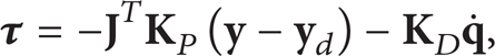
where
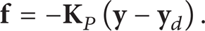
The force and torque can be controlled by
Figure 3 is a series of photographs of the experimental assembly sequence. As shown in panel (i), the robot holds on to the worksite with its right arm to compensate for any reaction force during the assembly. The robot installs the first component, member 1, during panels (ii) and (iii). The robot installs other members successively and assembles one truss unit, panels (iv)–(vi).
Control procedures for the assembly sequence are as follows. There are target markers in the experiment environment as shown in Figures 1 and 3. Target markers are located at the base of the truss structure and at the storage site for structural parts. Each target marker has three LEDs at triangular vertices. The vision system measures the marker position and orientation simultaneously. The robot recognizes the position of a part relative to the target marker before assembly. The robot places the end-effector position at the pick-up point, which is calculated from the target marker position as measured by the stereo vision system. At the pick-up point, the end-effector grasps a handgrip attached to the targeted part. The position and orientation of the part to the end-effector are settled uniquely when the end-effector grasps the handgrip. The robot plans the path of the arm and part to avoid collision with any other object in the work environment. It controls the arm to track along the planned path. The robot plans a path from the pick-up point to the placement point, avoiding obstacles by means of an artificial potential method [13]. Objects in the environment, for example, the truss under assembly, are regarded as obstacles. The arm is then directed along a planned trajectory by the sensory feedback control (1). The end-effector only makes contact with the environment when it picks up or places the part. Hence, feedback gains in (1) are chosen to make it a compliant control.
Consequently, the truss assembly task is successfully completed by control-based automation. However, measurement error in the vision system sensors, and so forth, prevents assembly from being guaranteed. Irrespective of uncertainties and variations at the worksite, the space robot model requires autonomy to complete the task goal.
4.2. Peg-in-Hole Task
The positioning control of (1) tries to complete the peg-in-hole task. The peg first is positioned at yθ = 0 [rad], it transits to the central axis of the hole, and it moves in a positive direction, toward
5. Existing Method for Autonomy with Reinforcement Learning
5.1. Outline of Existing Method with Reinforcement Learning
Reinforcement learning [1] is used to generate autonomous robot action.
In “standard” learning (Figure 6(a)), controller

Learning using (a) nominal plant model, (b) updated plant model, and (c) plant model with variation.
As shown in Figure 6(b), new plant model
If the robot cannot complete the task with the controller due to error between the model and the real plant, the robot switches to online learning. Adaptability is realized by online identification and learning. However, this cannot be used for peg-in-hole task, because online identification requires too much time. In the next section, a reinforcement learning problem for a peg-in-hole task requires several tens of thousands of state-action pairs. It requires tens of days for online identification if a hundred samples are selected for each state-action pair and each sampling takes one second.
5.2. Existing Method with Reinforcement Learning
5.2.1. Problem Definition
Following general dynamic programming (DP) formulations, this paper treats a discrete-time dynamic system in a reinforcement learning problem. A state s i and an action u k are the discrete variables and the elements of finite sets 𝒮 and 𝒰, respectively. The state set 𝒮 is composed of N s states denoted by s1, s2,…, s Ns and an additional termination state s0. The action set 𝒰 is composed of K actions denoted by u1, u2,…, u K . If an agent is in state s i and chooses action u k , it will move to state s j and incur a one-step cost g(s i , u k , s j ) within state transition probability p ij (u k ). This transition is denoted by (s i , u k , s j ). There is a cost-free termination state s0, where p00(u k ) = 1, g(s0, u k , s0) = 0, and Q(s0, u k ) = 0, ∀u k . We assume that the state transition probability p ij (u k ) is dependent on only current state s i and action u k . This is called a discrete-time finite Markov decision process (MDP). The system does not explicitly depend on time. Stationary policy μ is a function mapping states into actions with μ(s i ) = u k ∈ 𝒰, and μ is given by the corresponding time-independent action selection probability π(s i , u k ).
In this study, we deal with an infinite horizon problem where the cost accumulates indefinitely. The expected total cost starting from an initial state s0 = s i at time t = 0 and using a stationary policy μ is
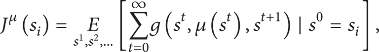
where E x [·] denotes an expected value, and this cost is called J-factor. Because of the Markov property, a J-factor of a policy μ satisfies

A policy μ is said to be proper if μ satisfies Jμ(s i ) < ∞, ∀s i .
We regard the J-factor of every state as an evaluation value, and the optimal policy μ* is defined as the policy that minimizes the J-factor:
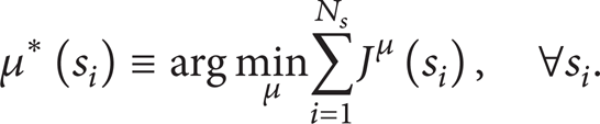
The J-factor of the optimal policy is defined as the optimal J-factor. It is denoted by J*(s i ).
The optimal policy defined by (5) satisfies Bellman's principle of optimality. Then, the optimal policy is stationary and deterministic. The optimal policy can be solved by minimizing the J-factor of each state independently. Hence, the optimal J-factors satisfy the following Bellman equation, and the optimal policy is derived from the optimal J-factors:

5.2.2. Solutions
The existing type of reinforcement learning problem is solved as “standard” learning in Figure 6(a). It obtains the optimal policy μnom*, which minimizes the J-factors of (7) for the nominal plant. It corresponds to controller
5.3. Learning Skill for Peg-in-Hole by Existing Method
5.3.1. Problem Definition of Peg-in-Hole
Here, the peg-in-hole task defined in Section 3.2.2 is redefined as a reinforcement learning problem.
State variables [y
x
, y
y
, yθ, f
x
, f
y
, fθ] in Section 3.2.2 are continuous but discretized into 1.0 [mm], 1.0 [mm], 0.5π/180 [rad], 2.0 [N], 1.0 [N], and 0.6 [Nm] in the model for reinforcement learning. The discrete state space has 4,500 discrete states, where the number of each state variable is [5, 5, 5, 4, 3, 3]. Robot action at the end-effector is u1, u2, u3, and u4, at each of the end-effector states transiting by ± 1 in the direction of the
Control in (1) is used to transit from present state s
i
to the next state s
j
by action u
k
. The reference manipulation variable to make the transition to s
j
is
The robot takes the next action after (1) control settles and the peg becomes stationary. Regardless of whether the peg is in contact with the environment, the robot waits for settling and proceeds to the next action. For this reason, state variables do not include velocity.
The goal is to achieve states with the largest y
x
, the peg position in
5.3.2. Learning Method
State transition probabilities for the state-action space in the previous section are calculated with sample data. Sample data are calculated with a dynamic simulator in a spatially continuous state space. The dynamic simulator is constructed with an open-source library, the open dynamics engine (ODE) developed by Russell Smith. The numerical model of this simulator has continuous space, force, and time in contrast to the discretized models for reinforcement learning in Section 5.2. This discretized state transition model is regarded as plant
5.3.3. Learning Result
The result of a numerical simulation in which controller

Trajectory of controller

Trajectory of controller
In an environment with the hole position error of −0.5 [mm] in
6. Autonomous Acquisition of Skill by Learning
6.1. Autonomous Acquisition of Skill for Peg-in-Hole
A robot can achieve peg positioning or movement with contact force, and it must have basic control functions same as a human being. Human vision measurement and positioning control are not accurate enough. However, the rate of a human failure in the same task is not as high as that of a robot. One reason for this may be the skills a human being brings to the task.
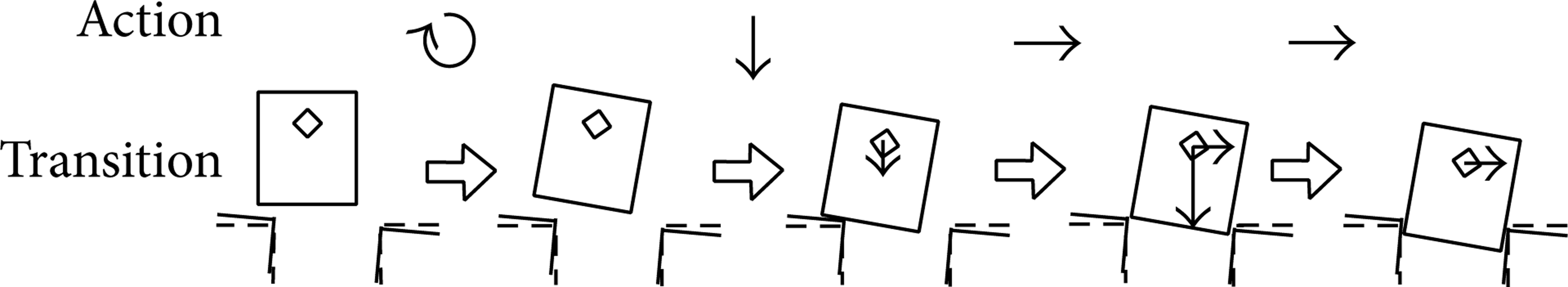
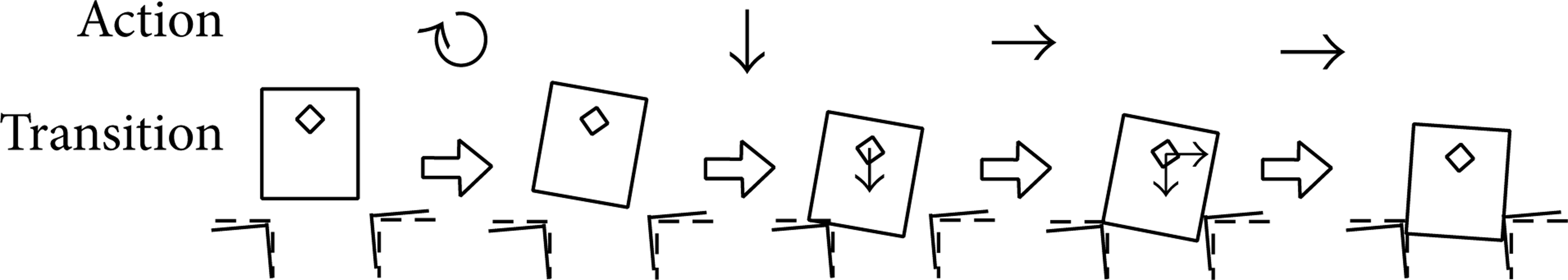
A human being conducting peg-in-hole task uses a typical sequence of actions (Figure 9). First, the human being puts a corner of the peg inside the hole. The peg orientation is inclined. The peg is in contact with the environment. Two points of the peg, the bottom and a side, are in contact with the environment, as shown in the close-up in Figure 9. The human then rotates the peg and pushes it against the hole and maintains the two contact points. The two corners are then inserted into the hole. Finally, the human inserts the peg into the hole and completes the task.
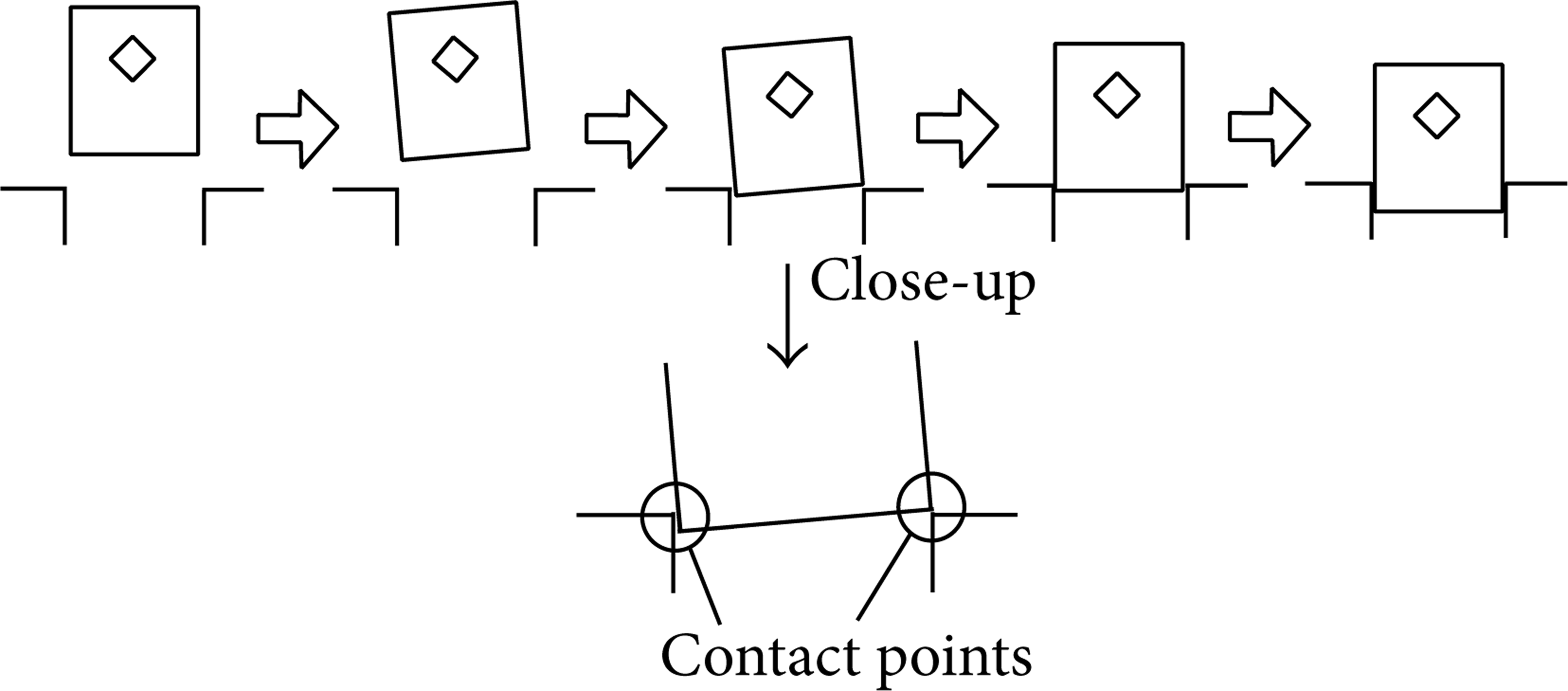
Human skill.
Human vision measurement accuracy and positioning control accuracy are not high. A human presumably develops skill while manipulating this situation. We conducted an experiment to check whether robot learning in the same situation could achieve the task as well as a human.
This situation conceptually corresponds to Figure 6(c). Plant
6.2. Problem Definition for Reinforcement Learning with Variation
We assume there are N variation plants around the estimated plant (the nominal plant). We use a set composed of N variation plants for learning.
We consider difference w l between a variation plant and the nominal plant in each state, which is a discrete variable and the element of finite set 𝒲. Finite set 𝒲 is composed of L differences denoted by w0, w1,…, wL − 1. Difference w0 indicates no difference. If an agent is in state s i with difference w l and chooses action u k , it will move to s j within a state transition probability p ij (u k ;w l ) and incur a one-step cost g(s i , u k , s j ;w l ). This transition is denoted by (s i , u k , s j ;w l ). Difference w l can be considered as the disturbance that causes state transition probability p ij (u k ;w0) to vary to p ij (u k ;w l ). We assume that the p ij (u k ;w l ) and g(s i , u k , s j ;w l ) are given.
Difference w l at each state is determined by a variation plant. Variation η is a function mapping states into difference with η(s i ) = w l ∈ 𝒲. The nominal plant is defined by η0(s i ) = w0 for all states s i . The plant does not explicitly depend on time, so variation η is time-invariant. We assume that η(s i ) = w l is given.
A plant set composed of N plants used for learning is represented by ℋ = {η0, η1,…, ηN − 1}. Set ℋ corresponds to {
For set ℋ, the expected cost of a policy μ starting from an initial state s0 = s i at t = 0 is

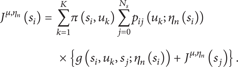
which is the J-factor of this problem. This J-factor formula using the plant existing probability is
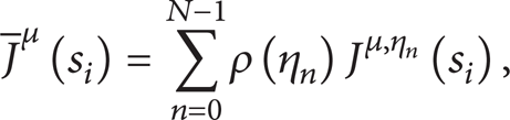
where
We define the optimal policy as
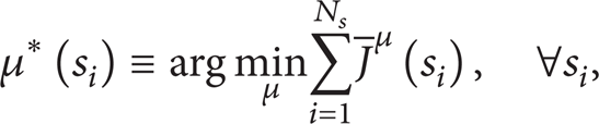
which minimizes the J-factor of every state. The J-factor of the optimal policy μ* is defined as the optimal J-factor, represented by
The variation plant in the original problem correlates with differences between any two states. Due to this correlation, the optimal policy does not satisfy Bellman's principle of optimality [14]. Therefore, the optimal policy and the optimal J-factor in this problem do not satisfy (6) and (7). In general, the optimal policy is not stationary. If policies are limited to stationary, the optimal policy is stochastic.
Therefore, another problem definition or another solution method is needed.
6.3. Solutions for a Relaxed Problem of Reinforcement Learning with Variation
We relax the original problem to recover the principle of optimality. Then, we can find the optimal J-factor efficiently by applying DP algorithms to the relaxed problem. We treat a reinforcement learning problem based on a two-player zero-sum game.
We assume that differences, w0, w1,…, w L , exist independently in each state s i . Then the original problem is relaxed to a reinforcement learning problem [15–17] based on a two-player zero-sum game [18] whose objective is to obtain the optimal policy for the worst variation maximizing the expected cost. Since the correlations of differences in a variation plant are ignored, the principle of optimality is recovered.
The ℋ2pzs is defined as the set of variation plants consisting of all possible combinations of any differences. Since each state has L types of differences, the number of variation plants in ℋ2pzs is
and the optimal J-factor J2pzs*(s i ) is defined as the J-factor of the optimal policy and the worst variation.
Since the principle of optimality is recovered, the optimal J-factor satisfies the following Bellman equation:
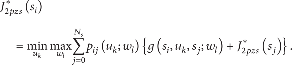
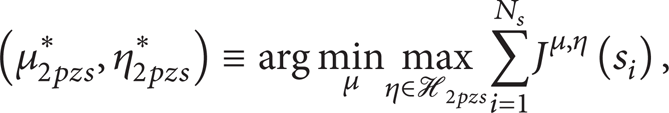
Therefore, the optimal J-factor can be obtained by a DP algorithm. Using the optimal J-factor, the optimal policy and the worst variation are obtained by

The optimal policy μ2pzs* is applicable to all
6.4. Learning of Peg-in-Hole Task with Variation
6.4.1. Problem Definition of Peg-in-Hole Task with Variations
This section uses the same problem definition for peg-in-hole as Section 5.3.1. The following is added to take variations into account.
The hole position and orientation are measured by the stereo vision system. These measurements involve errors caused by quantized images, lighting conditions at a worksite, and so forth. Time-averaged errors are almost constant while the space robot performs the task, unlike white noise whose time-averaged error is zero. Error evaluations are modeled as described below. Hole position errors are modeled as normal probability distributions, where the mean is m = 0 [mm] and standard deviation is σ = 0.75 [mm]. Hole orientation errors are modeled as normal probability distributions, where the mean is m = 0 [rad] and standard deviation is σ = 0.5π/180 [rad]. If the error's statistical values gradually vary, we have to estimate them online. The relative position and orientation between Σ0 and Σ hl are fixed during the task. The plant variations are modeled as hole position and orientation measurement errors.
Consider these errors as variations Δ
Hole position of variation plant η n from the nominal plant.

In the original problem, plant η n determines the state transition probability as p ij (u k ;η n ) for all state transitions (s i , u k , s j ) simultaneously. The state transition probability is represented by p ij (u k ;w n (s i )) where 𝒲(s i ) = {w0(s i ),…, wN − 1(s i )} and w n (s i ) = η n (s i ). On the other hand, the two-player zero-sum game allows difference w l at state s i to be chosen arbitrarily from 𝒲(s i ). The one-step cost is g(s i , u k , s j ;w l ) = 1.
In the later simulations and experiments to evaluate the learned results, the hole position and orientation are derived from the above normal probability distribution. In the simulations, a variation in the hole position and attitude is chosen for each episode, but the variation is invariant during the episode.
6.4.2. Learning Method
Under the conditions of the above problem definition, a policy is obtained by the solution in Section 6.3. It is the optimal policy μ2pzs* of the two-player zero-sum game, that is,
There is no proper policy for all plants in ℋ2pzs if the variations in Table 1 are too large. In this case, there is no policy satisfying the reinforcement learning problem based on the two-player zero-sum game. A typical approach for this situation is to make the variations smaller, to reconstruct ℋ2pzs, and to solve the two-player zero-sum game again. This approach is repeated if we cannot obtain any solutions. This approach reduces the robustness of solutions.
6.4.3. Control Results
In results for numerical simulation (Figure 10), where the peg arrives at the goal using controller

Trajectory of controller
The peg has arrived at the goal using controller
Trajectory of controller

Trajectory of controller

Trajectory of controller
Trajectory of controller
The task is achieved with controller
7. Evaluation of Obtained Skill
7.1. Results of Hardware Experiments
Example results in the hardware experiment using controllers

Experimental trajectories using two controllers in an environment with error (a) controller
7.2. Evaluation of Robustness and Control Performance
Robustness and control performance of controllers
Variation plants, that is, error in hole position and orientation, are derived from the normal probability distribution in Section 6.4. The robustness and the control performance are evaluated, respectively, by the task achievement ratio and the average step number to the goal. The achievement ratio equals the number of successes divided by the number of trials. Table 2 shows the achievement ratios and the average step number of
Achievement ratios and averaged step numbers of peg-in-hole task with controllers

Robust skills are thus autonomously generated by learning in this situation, where variations make task achievement difficult.
8. Conclusions
We have applied reinforcement learning to obtain successful completion of a given task when a robot normally cannot complete the task using controller designed in advance. Peg-in-hole achievement ratios are usually low when we use conventional learning without consideration of plant variations. In the proposed method, using variation consideration, the robot autonomously obtains robust skills which enabled the robot to achieve the task. Simulation and hardware experiments have confirmed the effectiveness of our proposal. Our proposal also ensures robust control by conducting learning stages for a set of plant variations.
Conflict of Interests
The authors declare that there is no conflict of interests regarding the publication of this paper.